e2
Accurate Capacitive Metrology for Atomic Force
Microscopy
by
Aaron David Mazzeo
Submitted to the Department of Mechanical Engineering
in partial fulfillment of the requirements for the degree of
Masters of Science
at the
MASSACHUSETTS INSTITUTE OF TECHNOLOGY
June 2005
©
Massachusetts Institute of Technology 2005. All rights reserved.
Author ...
...
Department of Mechanical Engineering
May 15, 2005
Certified by...
...
David L. Trumper
Professor
Thesis Supervisor
Accepted by ...
Lallit Anand
Chairman, Department Committee on Graduate Students
MASSACHUSETTS INSTITUTE OF TECHNOLOGY
Accurate Capacitive Metrology for Atomic Force Microscopy
by
Aaron David Mazzeo
Submitted to the Department of Mechanical Engineering on May 15, 2005, in partial fulfillment of the
requirements for the degree of Masters of Science
Abstract
This thesis presents accurate capacitive sensing metrology designed for a prototype atomic force microscope (AFM) originally developed in the MIT Precision Motion Control Lab. The capacitive measurements use a set of commercial capacitance sen-sors intended primarily for use against a flat target. In our design, the capacitance sensors are used with a spherical target in order to be insensitive to target rotations. The moving AFM probe tip is located approximately at the center of the spherical tar-get to make the capacitive sensing insensitive to the probe tip assembly's undesirable rotation on the order of 3 x 10- rad for 10 pim of lateral travel [48].
To accurately measure displacement of the spherical target relative to the ca-pacitance sensors, models for the caca-pacitance between a sphere and a circular disc were developed with the assistance of Katherine Lilienkamp. One of the resulting non-linear models was combined with the appropriate kinematic transformations to accurately perform measurement scans on a 20 pum x 20 pum surface with step heights of 26.5 nm. The probe tip positions during these scans were also calculated in real-time using Lilienkamp's non-linear capacitance model with a set of transformations and 3-D interpolation techniques implemented at 10 kHz. The scans were performed both in tapping and shear detection modes. Localized accuracy on the order of 1 nm with RMS noise of approximately 3 nm was attained in measuring the step heights. Surface tracking control and speed were also improved relative to an earlier prototype. Lateral speeds of approximately 0.8 pm/s were attained in the tapping mode.
In addition to improving the original prototype AFM's scan speed and ability to attain dimensional accuracy, a process for mounting an optical fiber robe tip to a
quartz tuning fork was developed. This mounting process uses Post-it notes. These
resulting probe-tip/tuning-fork assemblies were tested in both the tapping and shear modes. The tests in the tapping mode used the magnitude of the fork current for accurate surface tracking. The tests performed in the shear mode used the magnitude and phase of the fork current for accurate surface tracking.
Thesis Supervisor: David L. Trumper Title: Professor
Acknowledgments
I would not have been able to get through this Masters thesis without the help of
many supportive people. First and foremost, I would like to thank Professor David Trumper for his guidance and direction. He kept me on track and channeled my focus to ensure success. He taught me much about precision engineering and electronics. He constantly impressed me with his breadth of knowledge and expertise. In addition to working on atomic force microscopy, I am grateful for the opportunity I had to assist in teaching 2.003, one of my favorite courses as an undergraduate. His excellence and enthusiasm for teaching are contagious.
Next, I would like to thank Katherine Lilienkamp for her help and assistance in developing the key capacitance relationships necessary for accurate measurements. She stepped in out of curiosity and did more than I ever expected. She was very patient in explaining her results and ideas. Without her work the progress of this thesis would have been severely limited.
The work in this thesis would not have been possible without the initial AFM prototype built by Andrew Stein. I am very grateful for the time he put into leav-ing detailed information for followup work. When I had questions, he was kind in providing answers.
I would also like to thank Marcin Bauza and Professor Robert Hocken of
UNC-Charlotte for providing fiber optic probe tips. When our inventory of Stein's old tips began to dwindle, they quickly produced more probe tips for us.
I would like to thank Dr. Hans-Ulrich Danzebrink for supplying us with a diamond
probe tip mounted to a quartz tuning fork, along with a special holder. He inspired us to look at the tapping mode as an alternative to shear mode surface tracking.
MIT Professor Jacob White was also very helpful with respect to the numerical computation performed using FastCap. Through his lectures in 2.097J and a personal meeting, he was able to provide guidance and explain the usefulness of the boundary integral method.
for Manufacturing Machine Shop. Mark was great in helping me turn a couple of Stein's cone shaped targets into spherical targets.
Working in the Precision Motion Control Lab has been an educational and fulfilling experience thanks to Dave Otten, Marty Byl, Rick Montesanti, Xiadong Lu, Augusto Barton, Dave Cuff, Joe Cattell, Larry Hawe, Mart Corbijn van Willenswaard, and Twan Thomassen. Dave Otten had continued Stein's work before my arrival and was invaluable in helping me learn to operate the AFM. Not only did he teach me how to operate the AFM, but he was often willing to listen and make suggestions about possible improvements that could be made. Marty was very helpful in providing suggestions about Simulink, dSPACE, and signal processing. Rick lent me a hand with loop shaping and essential precision engineering techniques. Xiadong started wrapping aluminum foil around the wires in my experiment before I knew what was going on. He eliminated a lot of the noise in the system. Augusto, Dave Cuff, and Joe were great for idea bouncing and very helpful in answering car questions. Larry Hawe saved me lots of time by sharing some great macros for pdfTeX, along with some debugging experience. Mart Corbijn van Willenswaard and Twan Thomassen were visiting students from Eindhoven University of Technology, who explored the metrology concerns of the AFM with fervor. The "Dutch Dudes" also helped us get out of the lab and have a little fun.
Finally, I would like to thank my parents, siblings, and friends for their love and support. My roommates, Jared Casper, Otso Fristrom, and Steve Hatch were comic relief on a daily basis. Ashley Isaacson read and helped edit the entire thesis. My parents and little sister, Celeste, were always interested in my well-being and made sure my life outside the lab was productive and fruitful. Brian, my brother who is also graduating from MIT, spent more than a few hours either discussing or helping me solve problems I had with the AFM. He and his wife, Maren, have been kind, helpful, and close to campus. Jonina Allan, who is now in Spain, was also extremely supportive and patient in listening to my AFM woes. She helped me get through the Masters.
Contents
1 Introduction 29
1.1 Thesis Sum m ary . . . . 29
1.2 Atomic Force Microscopy and Our Prototype . . . . 33
1.3 Atomic Force Microscopy and Capacitive Sensing Applications . . . . 34
1.4 Implemented AFM Detection Methods . . . . 36
1.4.1 Shear Mode Surface Tracking . . . . 36
1.4.2 Tapping Mode Surface Tracking . . . . 37
1.5 Electromechanical Components . . . . 39
1.6 Thesis O verview . . . . 40
2 Capacitive Sensing 41 2.1 Capacitance Sensors . . . . 42
2.2 Capacitance Modeling . . . . 44
2.2.1 Capacitance between Spheres . . . . 44
2.2.2 Maxwell Capacitance Matrix . . . . 47
2.2.3 FastCap 2.0 Simulations . . . . 51
2.2.4 Katherine Lilienkamp's Numerical Methods . . . . 54
2.3 Evaluation of Capacitance Calculations . . . . 63
2.3.1 Capacitance Evaluations for Two Spheres . . . . 63
2.3.2 Capacitance Evaluation between a Sphere and a Grounded In-finite P lane . . . . 65
2.3.3 Capacitance Evaluation between a Sphere and a Flat Circular D isc . . . . 67
2.4 Capacitance Sensor Calibration . . . . 69
2.4.1 Mechanical Design . . . . 70
2.4.2 Determining Sensor Constants . . . . 73
3 AFM Design Modifications 77 3.1 Spherical Target Concept . . . . 77
3.1.1 Andrew Stein Kinematics . . . . 78
3.1.2 Kinematics for Spherical Target Design . . . . 81
3.1.3 Parametric Representation for Kinematic Interpolation . . . . 85
3.2 Hardware Modifications and Improvements . . . . 96
3.2.1 Spherical Target Machining . . . . 96
3.2.2 Tip M ounting . . . . 97
3.2.3 Initial Tip Mounting for Shear Mode Detection . . . . 99
3.2.4 Improved Tip Mounting for Shear Mode Detection . . . . 101
3.2.5 Tip Mounting for Tapping Mode Detection . . . . 104
3.2.6 Tapping Mode Assembly . . . . 106
3.2.7 Tip Centering . . . . 108
3.3 AFM Electronics . . . . 111
3.3.1 W iring . . . . 111
3.3.2 Tuning Fork Circuit . . . . 112
3.3.3 High Voltage Amplifier Modification . . . . 113
4 Real-time Implementation and Control 115 4.1 Real-time Position Interpolation . . . . 115
4.1.1 Simulink Implementation . . . . 116
4.1.2 Numerical Implementation . . . . 118
4.2 A FM Control . . . . 128
4.2.1 Lateral Control . . . . 130
4.2.2 Initial Shear Mode Detection with Thick Tips . . . . 133
4.2.3 Tapping Mode with Fork Decoupled from Piezo Tube . . . . . 141
5 Results 149
5.1 Shear Mode with Thick Probe Tip . . . . 149
5.1.1 Shear Mode Detection without Lateral Control . . . . 150
5.1.2 Shear Mode Tracking with Lateral Control . . . . 154
5.2 Tapping Mode Results . . . . 160
5.3 Shear Mode with Thin Probe . . . . 167
5.3.1 Fork Current Magnitude Detection . . . . 169
5.3.2 Fork Current Phase Detection . . . . 171
5.4 Linear-Non-linear Comparison . . . . 175
6 Conclusions and Suggestions 179 6.1 Sum m ary . . . . 179
6.2 Suggestions for Further Work . . . . 181
6.2.1 Capacitive Modeling . . . . 181
6.2.2 M etrology . . . . 182
6.2.3 Surface Tracking Sensor . . . . 183
6.2.4 Environmental Control . . . . 184
6.2.5 C ontrol . . . . 184
A Mechanical Drawings 187 B MATLAB Scripts 195 B.1 Lilienkamp Capacitance Calculations . . . . 195
B.1.1 find_poly-coeffs2 . . . . 195
B.1.2 capcalc-theory2 . . . . 197
B.2 Sensor-Sphere Position Determination Scripts and Functions . . . . . 199
B .2.1 find-gaps.m . . . . 199
B.2.2 gapifunc.2-sets-1.m . . . . 201
B.3 Kinematic Data Set Generation . . . . 207
List of Figures
1-1 Modified Figure 1-4 of AFM from Stein's thesis [48]. This photo shows
the housing and top view of the AFM. The micrometers are utilized to bring the probe tip close to the surface being scanned, and the optical view finder is used to roughly monitor the probe tip's location relative
to the surface being scanned . . . . 30
1-2 Cross-section view of the prototype atomic force microscope. The
probe tip displacement is monitored by a set of capacitance sensors surrounding a spherical target. The centerlines of the capacitance sen-sors are designed to intersect at the probe tip, which is nominally
coincident with the center of the spherical target. . . . . 31
1-3 Modified solid model depiction of the prototype AFM created by Stein.
This figure shows the quartz tuning fork and optical fiber probe tip
configuration. . . . . 32
1-4 The tuning fork oscillates horizontally relative to the scanning surface in the shear mode. The fork tracks the surface by remaining at a relative constant height. In this case, the fork also moves relative to
the stationary sample surface. . . . . 36
1-5 The spherical target is holding the tuning fork and probe tip for shear
mode scanning. The shielded wires are below the spherical target. . . 37
1-6 The tuning fork oscillates vertically relative to the scanned surface in
the tapping mode. In our prototype AFM's tapping mode, the tuning
2-1 Side view of a capacitance sensor relative to a spherical target. The minimum gap distance, g, and the lateral offset, a, determine the
ca-pacitance sensor output. . . . . 43
2-2 Scaled but undistorted side view of the capacitance probe related to the spherical target. The length of the probe line is 5 mm, and the radius of the sphere is 14.453 mm. The minimum gap offset g is 50
tim, and the lateral offset a is zero. . . . . 43
2-3 Two separated spheres of radius r1 and r2. The sphere centers 01 and
02 are separated by a distance d. The diagram is adapted from [45]
an d [18]. . . . . 45
2-4 Comparison of the capacitance between two spheres to the mutual capacitance between a sphere and a plane. These results were accom-plished using 1000 terms of Smythe's solutions with two spheres, each
having a radius of 1 m . . . . 50
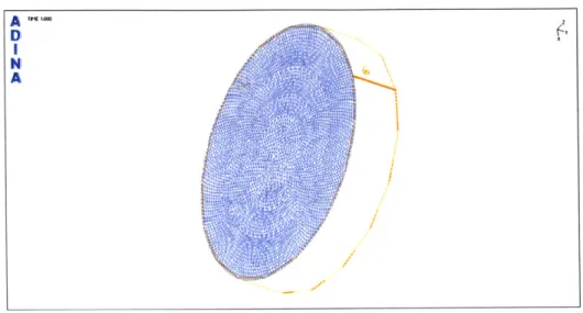
2-5 Disc created in ADINA as a face of a cylinder. This disc with a
diam-eter of 5 mm consists of 8776 triangular panels. The nodal coordinates and panel node number information are exported to a text file. Only
the meshed portion was used with FastCap. . . . . 52
2-6 Segment of a sphere created in SolidWorks and exported to ADINA
in parasolid format. This 20 degree revolved portion consists of 25188 triangular panels. The nodal coordinates and panel node information are exported to a text file. Only the meshed portion was used with
FastC ap . . . . 52
2-7 FastModel depiction of a sphere and disc separated by a distance of 300 [Lm. The spherical segment has 25188 panels, while the disc has 534. 53
2-8 FastModel depiction of a sphere, a disc, and an annulus. These surfaces
2-9 A graphical representation of Lilienkamp's resulting capacitance
rela-tionship between a sphere and a disc. The minimum gap distance g and the lateral offset a are given in units of meters. The linear capac-itance separation represents the equivalent gap distance between two parallel discs with diameters of 5 mm and no fringing effects. For these data the sphere had a radius of 0.01445 m, and the diameter of the
active portion of the disc for the capacitance sensor was 5 mm. ... 56
2-10 Side view depiction of the successive charge placement for the method of images capacitance calculation for the capacitance between a sphere and a circular disc with a corresponding infinite plane. . . . . 58
2-11 Resulting equipotential and electric field lines between a portion of a sphere and a grounded plane satisfying (2.26) and (2.28). This figure was created by Lilienkamp. . . . . 62
2-12 FastModel shows two spheres composed of 1224 elements each having a radius of 1 m. Their centers are separated by a distance of 3 m in this case. . . . . 63
2-13 The evaluated values for the Cu components of the Maxwell
capaci-tance matrix. The FastCap results agree reasonably well with the infi-nite series solutions derived by Maxwell and Smythe, but the Maxwell and Smythe solutions agree so well with each other that it is not pos-sible to distinguish them in this figure. Both spheres have radii of 1 m . . . . .. . . .. . . . . 64
2-14 The evaluated values for the C12 components of the Maxwell capaci-tance matrix by Maxwell, Smythe, Snow, and FastCap computation. In this figure, it is not possible to distinguish between the Smythe, Maxwell, and Snow solutions. Note that C12 < 0 by convention. . . . 65
2-15 Comparison of the solutions to the capacitance between two spheres to
the capacitance between a sphere and an infinite plane. The expression in (2.13) was used to compare the FastCap results in Figures 2-13 and 2-14 to Smythe's solutions for the capacitance between a sphere and a plane as shown in Figure 2-4. These results were accomplished using
1000 terms of Smythe's solutions. . . . . 66
2-16 C12 for the annulus, sphere, and disc combination compared to Lilienkamp's
numerical results. The annulus consisted of 5382 panels, the disc had
19952 panels, and the spherical target had 12544 panels. There was
zero lateral offset... . . ... . .. ... . . . . . 67
2-17 C12 interpolated error between Lilienkamp's results and the FastCap
results for the annulus, sphere, and disc combination. Earlier results in Figure 2-16 show the capacitance versus the minimum gap dis-tance. This figure shows measurement error in units of meters that we would expect to see if we were to use the FastCap solution in-stead of Lilienkamp's solution. Lilienkamp's results were taken as the absolute for this error analysis. . . . . 68 2-18 The linear calibration stage with accompanying solid model depiction.
A differential micrometer provides the actuation and moves the
spring-loaded carriage within the linear slide. . . . . 71 2-19 A close look at the assembled sensor calibration apparatus. A ball
coupling was used to interface the micrometer to the linear stage with-out over constraining the linear slide. The Heidenhain length gauge measurements were compared to the capacitance sensor measurements. 72
2-20 The calibration data was fitted to Lilienkamp's capacitance model us-ing her curve fittus-ing techniques. Each data point was taken manually. The lateral offset in this case was determined to be 494 pm. The standoff distance was determined to be 94.2 ptm for this probe. .... 73
2-21 The calibration data was fitted to Lilienkamp's capacitance model us-ing her curve fittus-ing techniques. The data points were taken in one sweep. The lateral offset in this case was determined to be 100 jim. The standoff distance was determined to be 94.1 tim for this probe.
This figure was produced by Lilienkamp. . . . . 74
3-1 Modified Figure 4-4 from Stein's thesis. The capacitance probes are
shown surrounding a cone shaped target [48] . . . .
78
3-2 Line scan of a Mikromasch TGZ02 calibration grating with step height
of 104.5 nm and pitch of 3.0 pm from Stein's data [48]. The measured
step height and pitch are too large by a factor of approximately 1.2. . 80
3-3 The conical target geometry overlaid on the spherical target. Radius
of the sphere is 0.569 in or 0.01445 m. . . . . 81
3-4 Diagram depicting a point P on the sphere a distance d from the
ca-pacitance sensor face and offset a distance a from the sensor centerline. Here, CP is perpendicular to the sensor face. The left half was taken
and modified from Figure 4-4 of Stein's thesis [48]. . . . . 82
3-5 A parametric representation of a line of probe tip travel from one corner
of a rectangular prism to the diagonally opposite corner. . . . . 86
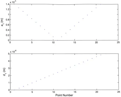
3-6 The minimum gap distance values, di, and the lateral offset values, a,
for capacitance sensor 1 are shown. These values are taken from the
data points shown in Figure 3-5. . . . . 87
3-7 The voltage outputs are given in units of meters via the capacitance
sensor scale factor of 0.2 V/pm with respect to a flat target. The out-puts represent the equivalent gap distance between two parallel discs
3-8 Parametric representation of a box of points. V was calculated using the appropriate sensor constant for sensor 1 as shown in Table 2.1. The estimated gap offsets for the spherical target at the measurement axes' origin used for the V calculation are from an AFM experiment
conducted on November 18, 2004. . . . . 89
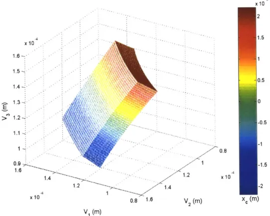
3-9 Parametric representation of V1, V2, and V3 in units of meters with a color map of x,. The estimated gap offsets for the spherical target at the measurement axes' origin used for the x, calculation are from an
AFM experiment conducted on November 18, 2004. . . . . 90
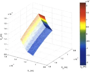
3-10 Parametric representations of V1, V2, and V3 with a color map for yc. The estimated gap offsets for the spherical target at the measurement axes' origin used for the y, calculation are from an AFM experiment
conducted on November 18, 2004. . . . . 91
3-11 Parametric representations of V1, V2, and V with a color map for z,. The estimated gap offsets for the spherical target at the measurement
axes' origin used for the z, calculation are from an AFM experiment
conducted on November 18, 2004. . . . . 91
3-12 The error between the initially created position coordinates and the
resulting position values when identical capacitance sensor output val-ues were used by the griddatan interpolation. The horizontal axis is the point number from the parametric representation, and there are
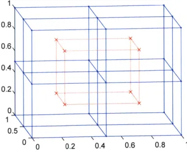
103275 points. . . . . 93 3-13 The x's on the corners of the inner box represent the test points used
in the second test of precision. . . . . 94
3-14 The error between the initially created position coordinates and the griddatan interpolated position values from the simulated capacitance sensor outputs for a set of position coordinates created according to the pattern shown in Figure 3-13. The horizontal axis is the point number from the parametric representation, and there are 92928 points. 95
3-16 Machined spherical target sitting on its partially turned fixture. . . . 96 3-17 Figure from Pohl's US patent 4,851,671. A pointed tip is mounted to
a piezoelectric crystal as part of a scanning microscope system [38]. . 97 3-18 Figure 4 from Karrai's US patent 5,641,896. An optical fiber is mounted
to a quartz tuning fork for use with a scanning microscope [27]. . . . 98
3-19 Different examples of optical fibers mounted to tuning forks. Photo
(a) shows an optical fiber from UNC-Charlotte mounted to a ECS-3X8 fork with an original resonance close to 32.768 kHz fork. This work was done by the author without a refined process. Photo (b) is from [6]. Photo (c) is from [41, 37]. Photo (d) is from [19]. . . . . 98
3-20 The Sutter Instrument P-2000 laser based micropipette puller was used
at UNC-Charlotte [2]. . . . . 99
3-21 Optical fiber tips produced by Bauza of UNC-Charlotte. The tips are
very thin and have a long taper. . . . . 100 3-22 Stereo microscope with two translation stages for target with
corre-sponding micrometers, a rotational stage, and a translation stage for the probe tip. . . . . 100 3-23 One of the first fork-tip assemblies we produced for shear mode
detec-tion. The optical fiber is one of the thicker, blunter tips produced by
Dr. Wang. The image was taken on July 15, 2004. . . . . 101
3-24 Optical fiber tip resting on a Post-it note. Image taken with the Intel
Play QX3+ with a magnification of 60X. . . . . 102
3-25 Fork, Post-it note, spherical target, and portion of assembly stage are
shown in the shear mode tip mounting process. The optical fiber probe is too small to be seen in this image. . . . . 103 3-26 Tuning fork with tip used on February 18, 2005 with our prototype
AFM to obtain accurate images. . . . . 104 3-27 Another view of the tip in Figure 3-26. . . . . 104
3-28 Fork attached to a different holder, which was glued to a spherical
target for tapping mode scanning. A relatively large metal tip is shown glued to the tuning fork. The metal probe was pulled off the Post-it
note. ... ... ...
3-29 This tapping mode fork with attached optical fiber tip was produced
using the block-Post-it method. . . . .
3-30 Tuning fork-tip assembly glued to a fixture attached to the spherical
target. . . . .
105
106
107 3-31 Photo of AFM in tapping mode with fork decoupled from piezo tube. 108 3-32 Probe tip centering device and modified spherical target. . . . . 109 3-33 Spherical target with probe tip centering device mounted on a PI spindle. 110
3-34 Three wire connections to the tuning fork are shown. Samples (a) and
(b) show thin, flexible wires. Sample (b) shows an attempt to shield
the wires with aluminum foil. Sample (c) shows two shielded cables running to the leads of the tuning fork. . . . .111
3-35 Tuning fork circuit with a voltage source and lock-in amplifier. . . . . 112
3-36 Modified version of Boudreau's high voltage amplifier. The five Apex PA88 operational amplifiers are visible. . . . . 114
3-37 Modified version of Figure 2-18 from Stein's thesis [48] showing the
changed compensating capacitor. . . . . 114
4-1 Real-time implementation of position determination in block diagram
form. The capacitance sensor outputs are shifted, scaled, rotated, and finally sent to lookup tables for interpolation. The results from the lookup table interpolation are the probe tip positions. . . . . 4-2 Identical system of points as shown in Figures 3-9 through 3-11 with
the majority of the points left out to facilitate viewing of the pb line segm ents. . . . . 4-3 Capacitance sensor outputs shifted to be centered about the origin.
The color map contains the x, component of the probe tip positions.
117
118
4-4 The shifted capacitance sensor outputs from Figure 4-3 have been ro-tated -44.9 (clockwise from above view) about the vertical V3 Shifted ax is. . . . . 120 4-5 The shifted and rotated capacitance sensor outputs from Figure 4-4
have been rotated -55.1' (clockwise according to right hand rule) about the horizontal V2 Rotated 1 axis. The number of points and surfaces
shown has been reduced for the sake of visibility . . . . 122 4-6 The rectangular interpolation set is embedded within the data set from
the twice rotated and shifted capacitance sensor outputs. 10000 points comprise the rectangular interpolation set, but the number of points shown is reduced for the sake of visibility . . . . . 123
4-7 The values for x, are given in the color maps. The rectangular inter-polation set has V and V2 domains from -18 pm to +18 pm and a V3
domain from -3.75 pm to +3.75 pm. . . . . 123
4-8 The values for ye are given in the color maps. The rectangular inter-polation set has V and V2 domains from -18 pm to +18 pm and a V3
domain from -3.75 pum to +3.75 tm. . . . . 124
4-9 The values for z, are given in the color maps. The rectangular inter-polation set has V and V2 domains from -18 pim to +18 pm and a V3
domain from -3.75 pum to +3.75 pm. . . . . 124
4-10 The position coordinate errors for xc, Yc, and z, using the shifted and twice rotated data set. The tested position values are a subset of the test points used in Figure 3-12. . . . . 125
4-11 The magnitude of the errors for xc, YC, and zc using the shifted and twice rotated data set. The tested position values are a subset of the test points used in Figure 3-12. . . . . 126
4-12 The position coordinate errors for xc, YC, and z, using the shifted and twice rotated data set. The tested position values are a subset of the test points used in Figure 3-14. . . . . 127
4-13 The magnitude of the errors for xc, yc, and ze using the shifted and twice rotated data set. The tested position values are a subset of the
test points used in Figure 3-14. . . . . 127
4-14 High-level block diagram for the metrological AFM's control system. Two lateral scanning controllers are used to control the probe tip's position in the horizontal plane, while an axial height regulation system closes the loop on the tuning fork proximity sensor signal to maintain a constant probe-sample gap. This diagram is similar to Figure 5-1 in
Stein's thesis [48.
. . . .
129
4-15 A simplified block diagram created by Stein (Figure 5-4 in his thesis)for the X scanning loop [48]. The Y loop is virtually identical. . . .. 130
4-16 Measured open loop frequency response for the X scanning loop. A lightly damped resonant peak is observed at 960 Hz, which corresponds to the tube scanner's bending mode. The blue line is the theoretical
open loop model fitted to the data. . . . . 131
4-17 Block diagram for the X plant and lateral scanning controller, which consists of an integrator in series with a low-pass filter (see (4.4)). The
same controller is used for Y. . . . . 132
4-18 Measured closed loop frequency response for the X scanning loop. The
lateral control system has a -3 dB crossover frequency of 198 Hz. . . 132
4-19 A simplified block diagram for the axial height regulation system, which shows blocks containing the key components for surface track-ing or axial height regulation. This figure is similar to Figure 5-15 in
Stein's thesis [48]. . . . . 134
4-20 Diagram depicting the setup for determining the plant dynamics. . . 134
4-21 Frequency response of the probe tip-surface interaction for shear mode sensing. The reference current was set to 75% of the maximum current
(3.75 nA /5 nA ). . . . .
135
4-23 Theoretical and measured closed loop response of the integral con-troller with unity gain for shear mode height tracking, along with the theoretical negative of the loop transmission. . . . . 137
4-24 The closed loop response of the integral-lead controller with a gain of
1.61 for shear mode height tracking, along with the negative of the
loop transmission of the integral-lead controller in conjunction with the axial height regulation plant. . . . . 138
4-25 The closed loop response (shear mode) of the integral-lead controller with a model gain of 1.61 and an actually implemented gain of 2.5 for shear mode height tracking. . . . . 139
4-26 Measured and fitted open loop frequency response data for the height tracking system in tapping mode. . . . . 142 4-27 Measured and theoretical closed loop frequency response data for the
height tracking system, along with the theoretical negative of the loop transm ission. . . . . 143 4-28 Frequency response of the fork current phase versus the vertical
com-mand signal, u,. These data were collected using a thin probe tip. . . 146
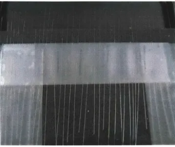
5-1 Resulting scan of a MikroMasch silicon grating TGZO1 sample using the shear tracking mode and similar probe tips used by Stein in earlier experiments. The dashed lines indicate fitted lines to the x-z and
y-z coordinates of the data. The original scan (data acquisition) was
performed on August 11, 2004 . . . . 151
5-2 Shear mode tracking scan flattened by two rotations. The original data are shown in Figure 5-1. . . . . 152 5-3 Side views of shear mode tracking scan. The upper trace consists of
all the data points shown in Figure 5-2 projected into the x-z plane. The lower trace is the same data projected into the x-y plane. . . . . 152
5-4 One portion of the flattened shear mode tracking scan shown in Fig-ure 5-2. The upper trace is a portion of one line scan projected into the x-z plane. The lower trace shows the lateral motion of the line
scan in the x-y plane. . . . . 153
5-5 Scan from October 13, 2004 shows the raw data from the real-time
interpolation for the shear mode tracking with lateral control. The upper data set is from capacitance sensors 4, 5, and 6. The lower data set is from sensors 1, 2, and 3. . . . . 155
5-6 The difference between the MATLAB interpolation of the position data
from capacitance sensors 1, 2, and 3 and the dSPACE real-time im-plementation. These results are purely numerical and show that the linear interpolation used by dSPACE is virtually identical to the linear
interpolation performed by the MATLAB interp3 function. . . . . . 156
5-7 Shear mode tracking scan with lateral control flattened by two
rota-tions. The original data are from sensors 1, 2, and 3 as shown in Figure
5-5. The self-calibration spikes have been removed. . . . . 157
5-8 One line of the flattened scan for shear mode operation with lateral
control shown in Figure 5-7. The upper trace shows the line scan data projected into the x-z plane. The lower trace shows the line scan data
lateral movement in the x-y plane. . . . . 158
5-9 AFM scan performed on October 12, 2004 in the shear mode with a
relatively large driving voltage of 22.8 mVpp at the tuning fork electrodes. 159
5-10 Portion of the AFM scan shown in Figure 5-9. The pitch is
approxi-mately 3.1 ym, but the valleys are too narrow. The measured plateau
width in the scan is approximately 2.5 pm. . . . . 160
5-11 Tapping mode scan with lateral control from November 9, 2004. The
scan was flattened by two rotations, and the self-calibration peaks were
5-12 One line of the tapping scan with lateral control shown in Figure 5-12.
The upper trace is the line segment projected into the x-z plane, while the lower trace shows the line segmented projected into the x-y plane. 162
5-13 Side views of the tapping mode scan shown in Figure 5-11. The upper
trace shows the data projected into the y-z plane. In the y-z projection, the probe tip can be conceptualized as having moved from the left side to the right side during the two hour scanning period. The lower trace shows the lateral movement of the probe tip in the x-y plane. . . . . 163
5-14 Tapping mode scan with integral surface tracking control. Time re-quired for scan was two hours. Abberation (fiducial mark) in upper
right hand portion of scan is visible. . . . . 164
5-15 Tapping mode scan with integral and double lead tracking control.
Time required for scan was ten minutes. The aberration (fiducial mark) in the upper right-hand portion of the scan is visible and more pro-nounced in this image than in Figure 5-14. . . . . 165
5-16 Side views of the tapping mode scan shown in Figure 5-15. The top
trace shows the data projected into the x-z plane, the middle trace shows the data projected into the y-z plane, and the bottom trace shows the lateral motion of the probe tip in the x-y plane. . . . . 166
5-17 Portion of the tapping mode scan shown in Figure 5-15. The upper
trace is the data projected into the x-z plane. In this view, slight curvature is observed over the 20 pm span. The lower trace shows the lateral motion of the probe tip in the x-y plane. . . . . 166
5-18 Another ten minute tapping mode scan performed on February 4, 2005.
5-19 Side views of another tapping mode scan performed in ten minutes.
The data were taken from Figure 5-18. The top trace shows the data projected into the x-z plane, the middle trace shows the data projected into the y-z plane, and the bottom trace shows the lateral motion of the probe tip in the x-y plane. These views were used to verify the
flatness of the rotated data. . . . . 168
5-20 Side views of a portion of the scan in Figure 5-18 after the two rotations
were applied. The upper trace is the line segment projected into the x-z plane, while the lower trace shows the line segment projected into
the x-y plane. . . . . 169
5-21 3-D view of a shear mode scan taken with a thin optical fiber. The
scan was executed on February 21, 2005, and the magnitude of the fork
current was used for surface tracking. . . . . 170
5-22 Side views of the scan in Figure 5-21. Two rotations were applied.
The top trace shows the data projected into the x-z plane, the middle trace shows the data projected into the y-z plane, and the bottom trace
shows the lateral motion of the probe tip in the x-y plane. . . . . 170
5-23 Side views of one portion of the scan shown in Figure 5-21. The upper
trace shows the line data projected into the x-z plane. The lower trace shows the lateral movement projected into the x-y plane. Slight distur-bances in the lateral motion are observed as the probe tip encounters
the grating steps. . . . . 171
5-24 3-D view of a shear mode scan using the phase of the fork current for
surface tracking. The scan was performed on February 23, 2005. . . . 172
5-25 Side views of the scan shown in Figure 5-24. The top trace shows the
data projected into the x-z plane, the middle trace shows the data projected into the y-z plane, and the bottom trace shows the lateral
5-26 Side views of a line portion of the scan in Figure 5-24. The upper
trace shows the line data projected into the x-z plane. The lower trace shows the lateral movement projected into the x-y plane. . . . . 174
5-27 Simulated scan image using a linear transformation for position
cal-culations without the non-linear capacitance relationships or modified kinem atics. . . . . 175 5-28 Same region shown in Figure 5-17 with a comparison between results
from the modified transformation-interpolation method and results us-ing the linear transformations from the initial AFM prototype. The middle two panels show the same results shown in the top panel and are included to distinguish the two traces apart without color printing. The bottom panel shows the lateral movement of the probe tip. The upper trace in the bottom panel is from the new modified AFM com-putational results, while the lower trace in the bottom panel is from the linear transformations of the original prototype. . . . . 177
A-1 Sheet 1 of the modified spherical target. This drawing is a modified
version of Stein's cone shaped target. . . . . 188 A-2 Sheet 2 of the modified spherical target. This drawing is a modified
version of Stein's cone shaped target. . . . . 189 A-3 Drawing of the inner cylindrical target shown in Figure 3-32, which was
never machined. This drawing could be used for a future tip centering
d ev ice. . . . . 190
A-4 Sheet 1 of the modified spherical target shown in Figure 3-32, which was never machined. This drawing could be used for a future tip centering device. . . . . 191 A-5 Sheet 2 of the modified spherical target shown in Figure 3-32, which
was never machined. This drawing could be used for a future tip centering device. . . . . 192
A-6 Sheet 1 of the modified spherical target shown in Figure 2-18, which
was used for capacitance sensor calibration to Lilienkamp's numerical
m odel. . . . .. . . . . . 193
A-7 Sheet 2 of the modified spherical target shown in Figure 2-18, which
was used for capacitance sensor calibration to Lilienkamp's numerical
List of Tables
2.1 Sensor standoff distances (sensor constants) determined for the six
AFM capacitance sensors. . . . . 75
Chapter 1
Introduction
1.1
Thesis Summary
In this thesis, we present the application of accurate capacitive sensing metrology to displacement measurements of a spherical target. To demonstrate the accurate capacitive sensing metrology, we show resulting images from our prototype atomic force microscope (AFM) with the integrated capacitive sensing. The original proto-type AFM was built by Andrew Stein [48], and we outline our modifications to the hardware, control, and data processing of his original prototype. A picture of the original prototype AFM is shown in Figure 1-1.
In both the new and old versions of the prototype AFM, a set of capacitance sensors were used for monitoring the displacement of an optical fiber probe tip as scans were performed. These capacitance sensors surrounded a target with an embedded tuning fork oscillator. Attached to one of the tines of the tuning fork was the optical
fiber probe tip. This probe tip-tuning fork assembly was responsible for tracking sample surfaces. By accurately tracking a calibration grating surface with the probe tip-tuning fork assembly, we were able to verify the precision measurements of the AFM and the capacitive sensing metrology.
In the initial prototype built by Stein [48], the capacitance target was cone shaped. For the new prototype, we replaced the cone shaped target with a spherical target. This spherical target with the other main components of the AFM assembly is shown
in Figures 1-2 and 1-3. As shown in these figures, the spherical target was attached
to a piezo tube, which provided actuation. During a scan the piezo tube moved the
spherical target and probe tip laterally and vertically with three degrees of freedom.
Mo
e
te
icrometers
AFM housing Optical
viewfindr -Capacitance
p
sensors
Figure 1-1: Modified Figure 1-4 of AFM from Stein's thesis [48]. This photo shows the housing and top view of the AFM. The micrometers are utilized to bring the
probe tip close to the surface being scanned, and the optical view finder is used to
roughly monitor the probe tip's location relative to the surface being scanned.
With lateral motion of the probe tip due to piezo tube actuation, there was
in-herent rotation of the capacitance target. This rotation, combined with the lack of a
non-linear capacitance model for the cone shaped target, lead to measurement errors
in the original prototype. For the new prototype we converted the cone shaped target
into a spherical target and created the necessary capacitance model and kinematic
transformations to accurately monitor the displacement of the spherical target
rel-ative to its surrounding capacitance sensors. If the probe tip were at the center of
the spherical target, the probe tip's position relative to the spherical target's surface
would be insensitive to rotation, and the measurement error due to rotation induced
by the piezo tube would be eliminated. Our probe tips were placed near the center
sufficient time to implement a precise tip centering design described in Section 3.2.7. To accurately monitor the displacement of the probe tip, we created a model for the capacitance between a sphere and a flat circular disc with the assistance of Katherine Lilienkamp. We then implemented the results of this capacitance model with a new kinematic model to relate the output of the capacitance sensors to the motion of the spherical target. This kinematic model implementation was verified by scanning calibration surfaces with specified dimensions.
In addition to modifying the capacitive sensing metrology, we made modifications to the control and surface tracking components to produce more accurate scan images. The original prototype operated in the shear mode (see Section 1.4.1). We were able to increase the scan speed and eliminate some measurement drift by reconfiguring the microscope to operate in the tapping mode, which is explained in Section 1.4.2.
Capacitance Sensors
-30
mm ->
Piezo Tube
Pobe Tip
Quartz Tuning Fork
Spherical Target
Figure 1-2: Cross-section view of the prototype atomic force microscope. The probe tip displacement is monitored by a set of capacitance sensors surrounding a spherical target. The centerlines of the capacitance sensors are designed to intersect at the probe tip, which is nominally coincident with the center of the spherical target.
In our final experiments, we ran the microscope in the shear mode and experi-mented with using phase instead of magnitude for surface tracking (see Section 4.2 for general overview on magnitude or phase surface tracking). When using a very thin probe tip in the shear mode for a few scans, the phase of the fork current was more useful than the magnitude in obtaining accurate images. Using the phase instead of the fork current also appeared to limit measurement drift in the vertical direction.
If more time had been available, we could have gone back to the tapping mode and
experimented with the use of phase for surface tracking.
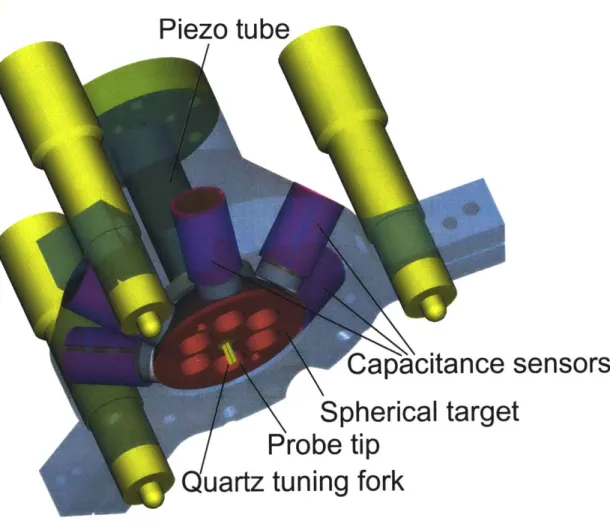
Piezo tube
A
apacitance sensors
Spherical target
Probe tip
uartz tuning fork
Figure 1-3: Modified solid model depiction of the prototype AFM created by Stein. This figure shows the quartz tuning fork and optical fiber probe tip configuration.
1.2
Atomic Force Microscopy and Our Prototype
The atomic force microscope (AFM) traces its origin to Binnig [12], which grew out of the scanning tunneling microscope originally developed by Rohrer and Binnig
[13]. Atomic force and scanning tunneling microscopy both maintain a probe tip a
constant distance from the surface being scanned. The scanning tunneling microscope (STM) monitors the current flowing through the electron cloud between the tip and a conductive surface to regulate a constant tracking height. The STM requires a conductive sample to function properly. The AFM is different from the STM in that it detects changes in interatomic forces between a probe tip and a surface to regulate a constant tracking height. By using interatomic forces and not tunneling current, the AFM does not require a conductive sample surface.
To successfully track a surface and regulate a constant tracking height, some AFMs use an oscillating micro-cantilever beam with a sharp probe at the end. The backside of the cantilever has a reflective surface for use with optical position sensing.
A laser is aimed at the end of the cantilever, and the beam reflects off the backside
of the cantilever and into a photodetector. By analyzing the light received by the photodetector, it is possible to determine whether a force has been applied to the end of the tip by monitoring the tip displacement. For proper height tracking, the goal is to maintain the deflection of the cantilever beam at a constant value while scanning
[26].
Another method for surface tracking employs the use of a quartz tuning fork with an attached probe tip. The tuning fork is either excited mechanically through the use of a dithering piezo electric device as described in [54] or electrically as described in [52, 21]. In our prototype AFM, we used an electrically excited tuning fork with an optical fiber probe tip. We experimented with optical fiber probe tips because we were able to work with Professor Robert Hocken of UNC-Charlotte to obtain tips with an end radius on the order of 1 pm. These probe tips were also initially used in Hocken's group to explore near-field scanning optical microscopy (NSOM), although our tips were cut short and not used as optical sensors.
In general, the probe-tip proximity sensor may be held fixed as the surface moves relative to the sensor, or the proximity sensor may be attached to the actuator, while the probe moves relative to the surface. In our prototype AFM, we initially operated with a moving probe and fixed surface for shear mode scanning. Later, we demonstrated accurate measurement results with a fixed probe and moving surface in the tapping mode.
In either the shear or tapping modes (see Section 1.4 for detailed descriptions), a fine probe tip is interacting with a surface. Work has been done by others to describe the associated weak force interactions. At least a portion of the interactive forces between a probe tip and a metal surface may be described in terms of capacitance as shown in [24]. Jalili also reviews a variety of proposed models of differing complexi-ties in [26]. With respect to the control implementation in our prototype AFM, we did not design our controllers based on any of these models. We performed our sur-face tracking control via loop shaping based upon experimentally-determined probe dynamics.
For more information concerning the history and origins of atomic force mi-croscopy, see Section 1.3.1 of Stein's thesis [48]. Stein's thesis also contains an abun-dance of information concerning the initial prototype AFM.
1.3
Atomic Force Microscopy and Capacitive
Sens-ing Applications
Atomic force microscopy has become an integral measuring device to the semicon-ductor and MEMS industries. In the semiconsemicon-ductor and MEMS industries, AFMs are used for surface roughness evaluations as well as accurate dimensioning of surface features. Outside the semiconductor and MEMs fields, AFMs have also been applied to the analysis of biological systems.
One very impressive AFM application has been developed by Toshio Ando's group of the Kanazawa Biophysics Lab at Kanazawa University in Japan. Using high-speed
AFM technology that they developed, they have been able to record movies of kinesin moving along a microtubule, ATP reacting to ultraviolet light, and a myosin molecule changing shape. They use a cantilever beam and fine probe tip in tapping mode for surface tracking in aqueous solutions. In order to increase the movie frame rate, they have improved the individual components of their overall system. A couple of these components include the cantilever beam sensing device and the moving stages. Ando's macromolecule movies are one example of how atomic force microscopy has affected biology and will continue to do so [9, 8, 7].
While our prototype AFM does not have the imaging speed exhibited by Ando's microscope, our prototype AFM is uniquely designed to use a set of capacitance sensors with a spherical target for both the lateral and vertical position measurements of the probe tip motion. We do not use laser interferometry for any measurements. We also do not rely on a piezo tube characterization for position information. The piezo tube only provides the actuation. This project's greatest contributions lie in the accurate capacitive sensing metrology and the real-time displacement measurements using this metrology.
Capacitive sensing has been used in many precision engineering applications. Of-ten capacitance sensors are used with a flat target to measure axial motion. However, they can also be found in applications with rounded surfaces. One application is in measuring the roundness of precision spheres [20]. Another, more common application is for spindle measurements. In [49], Swann, Harrison, and Talke used capacitance sensors for their analysis of non-repeatable runout for fluid lubricated spindles. In [46], Srinivasa, Ziegert, and Mize used a laser ball bar for measuring thermal drift, but they still made comparisons with capacitive sensing results. In [46, 49], the ca-pacitance sensors were used with a cylindrical target. In many cases, a standard capacitance sensor calibrated for a flat surface may be used with a cylindrical target as long as the radius of the target is large enough or the radius of the probe is small
enough [4].
If someone is interested in performing spindle measurements using a round ball as a capacitance target, the results of this thesis will be very useful. With the capacitance
and kinematics modeling outlined in this thesis, it is possible to accurately measure displacement of a sphere surrounded by a set of capacitance sensors. Some additional work and testing would need to be done, but the concepts in this thesis are directly applicable.
1.4
Implemented AFM Detection Methods
The atomic force microscope in the Precision Motion Control Lab was tested in two detection modes: shear and tapping. These modes of operation were dependent on the fork-scanning surface orientation. In the shear mode, the probe tip was coupled to the motion of the piezo tube. In the tapping mode, the fork was stationary, while the surface being scanned was attached to the piezo tube.
1.4.1
Shear Mode Surface Tracking
Shear mode scanning was the standard detection method for Stein's prototype atomic force microscope. In this form of atomic force microscopy, the probe tip oscillates horizontally very close to the surface being scanned. Figure 1-4 depicts the basic shear detection mode.
Wires
Probe
Tuning Fork
Surface
Figure 1-4: The tuning fork oscillates horizontally relative to the scanning surface in the shear mode. The fork tracks the surface by remaining at a relative constant height. In this case, the fork also moves relative to the stationary sample surface.
For the shear detection mode we glued the tuning fork in a circular hole of the spherical target with an orientation perpendicular to the surface being scanned. The tuning fork leads were inserted into a pair of sockets, which were connected to shielded wires to avoid noise due to stray capacitance. Figure 1-5 shows the spherical target with the fork connected to the shielded cables.
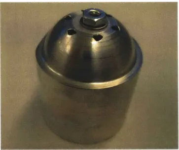
Figure 1-5: The spherical target is holding the tuning fork and probe tip for shear mode scanning. The shielded wires are below the spherical target.
1.4.2
Tapping Mode Surface Tracking
The tapping mode has been used by many people to obtain accurate surface images.
A graphical depiction is shown in Figure 1-6. In this case, the oscillatory motion of
the tuning fork is perpendicular to the surface being scanned. In our prototype AFM, we mounted the sample surface to the moving spherical target and fixed the quartz tuning fork to the microscope base. During a tapping mode scan, the sample surface moved relative to the fixed tuning fork.
Before we ran the AFM in the tapping mode with the sample moving relative to the tuning fork, we had the tuning fork mounted to the bottom of the spherical target in a flipped orientation from that shown in Figure 1-6. However, we were unable to perform image scans and encountered the problems described in Section 3.3.3 with the unstable high voltage amplifier exciting the piezo tube and tuning fork. At the time, we did not know that the high voltage amplifier was unstable, but we did witness a large amount of noise on the tuning fork signal. In an effort to reduce visible noise on the tuning fork signal, we decoupled the tuning fork from the piezo tube motion (fixed the tuning fork to the AFM base). Shortly after decoupling the tuning fork and the piezo tube motion, we debugged/stabilized the high voltage amplifier. We then obtained our fastest scans in the tapping mode with the tuning fork decoupled from the piezo tube motion.
Surface
Wires
Probe
Tuning Fork
Figure 1-6: The tuning fork oscillates vertically relative to the scanned surface in the tapping mode. In our prototype AFM's tapping mode, the tuning fork was fixed, while the surface moved.
With limited time remaining to complete this thesis, we did not see the value in swapping the positions of the probe and surface to have a moving probe relative to a stationary surface. That said, we believe the the microscope would have been able to obtain accurate scans in the tapping mode with a moving probe. However, without significant changes to the controller, it is doubtful that the surface tracking would have been faster than the speed attained with the tested tapping mode configuration.
1.5
Electromechanical Components
The majority of the electromechanical components used by Stein were retained and used throughout this project. Throughout this thesis, we make reference to these components, and this section provides a brief listing of them and their use in the project. For the real-time control and signal processing, a dSPACE DS1103 PPC Controller Board was used in conjunction with Windows XP, MATLAB 6.5.1 Release
13 (Service Pack 1), Simulink, and dSPACE ControlDesk 2.4. This DSP board was
used in an Intel Pentium IV personal computer. The computer processed data from
ADE Technologies 2805 passive capacitance sensors with ADE Technologies 3800
gaging modules. These capacitance sensors monitored a target subject to actuation
by a piezoelectric tube from PI Ceramic (PT-130.24). The voltage drive to the piezo
tube was provided by a modified version of a five channel high voltage amplifier (+/-100 Volts) originally built by Brian Boudreau while he was at UNC-Charlotte working
on a PhD from Michigan Technological University. The vertical actuation of the piezotube was controlled by various quartz tuning fork-optical fiber proximity sensors. These proximity sensors consisted of an optical fiber tip furnished by UNC-Charlotte glued to one tine of an ECS-3X8 32.768 kHz quartz tuning fork (a standard watch crystal with the end of the package removed). The feedback signal for the vertical actuation was provided by a Stanford Research Systems SR530 Lock-in Amplifier, which synchronously detected the current through the quartz tuning fork. The tuning fork sinusoidal driving voltage was provided by an HP 33120A Arbitrary Waveform Generator.
As mentioned before, most of the electromechanical components were used by Stein in the original prototype. However, electrical, mechanical, and computational changes were made. Computational models were developed to compensate for the new spherical target being used in conjunction with the capacitance sensors. An important electrical modification was made to the high voltage amplifier. Mechanical modifications were made to the cone shaped target (machined into a spherical shape) used by the capacitance sensors, the proximity sensor holding and orientation, and
the tuning fork assembly. With respect to the tuning fork assembly, we also developed a new tip mounting procedure.
1.6
Thesis Overview
The remainder of this thesis is organized as follows: In Chapter 2, we outline the theory, some infinite series solutions, and numerical solutions to solve for the capaci-tance between a sphere and a flat disc. Katherine Lilienkamp contributed greatly to the work therein. In Chapter 3, we discuss the kinematics and numerics that describe the motion of the AFM spherical target and probe tip relative to the capacitance sensors. We also present the AFM hardware modifications, including a novel method for mounting an optical fiber probe tip to a quartz tuning fork using a Post-it® note. In Chapter 4, we present the additional numerics necessary for real-time displace-ment measuredisplace-ments and the control methods for lateral motion and surface tracking. In Chapter 5, we present a number of scans and show that our AFM has localized accuracy on the order of a few nanometers in the vertical direction. In Chapter 6, we conclude this thesis and make suggestions for additional work.
Chapter 2
Capacitive Sensing
Katherine Lilienkamp developed numerical capacitance relationships for the working AFM. The content in Sections 2.2.4 and 2.4.2 of this chapter involving the capacitance between a sphere and a circular disc is a result of her research. Comparable infor-mation from this chapter is currently being developed into an article by Lilienkamp, Mazzeo, Corbijn van Willenswaard, Thomassen, and Trumper [28].
Generally speaking, capacitance sensing has been utilized to achieve sub-nanometer measuring resolution. The ability to achieve sub-nanometer resolution makes capac-itive sensors a viable alternative to laser interferometry for many precision measure-ment applications, where the range of travel is relatively small.
We attempted several numerical approximations to solve for the capacitance be-tween a sphere and an infinite plane or a flat circular disc. The first numerical method we explored satisfies Laplace's equation using the multipole integral equation method implemented in FastCap 2.0 software [36]. Another set of solutions is based on infi-nite series approximations by Smythe [44] and Maxwell [33]. The method we actually implemented with our AFM involves iteratively approximating electric field lines to satisfy Laplace's equation.
![Figure 3-1: Modified Figure 4-4 from Stein's thesis. The capacitance probes are shown surrounding a cone shaped target [48].](https://thumb-eu.123doks.com/thumbv2/123doknet/13828217.443064/78.918.192.719.446.740/figure-modified-figure-stein-thesis-capacitance-probes-surrounding.webp)
![Figure 3-20: The Sutter Instrument P-2000 laser based micropipette puller was used at UNC-Charlotte [2].](https://thumb-eu.123doks.com/thumbv2/123doknet/13828217.443064/99.918.250.658.510.861/figure-sutter-instrument-laser-based-micropipette-puller-charlotte.webp)