Adaptive Frequency Modulation
for Satellite Television Systems
RLE
Technical Report No. 554
April 1990
Julien Piot
Research Laboratory of Electronics Massachusetts Institute of Technology
Cambridge, MA 02139 USA
This work was sponsored in part by the Advanced Television Research Program, the Graff Inst. Company Fellowship, the Hasler Foundation, Switzerland, the Swiss
.National Fund for Research, and by the Brown Bovery Corporation, Switzerland.
Adaptive Frequency Modulation
for Satellite Television Systems
by Julien Piot Submitted to the
Department of Electrical Engineering and Computer Science
on January 10, 1990 in partial fulfillment of the requirements for the Degree of Doctor of Philosophy in Electrical Engineering
Abstract. Frequency modulation is the first choice coding scheme in many existing
applications such as satellite television transmission.
A simple model of image formation predicts large variations in the short-time bandwidth of the modulated signal. Based on this model, the frequency deviation in a small block of the picture is adjusted in order to keep the bandwidth constant. The resulting noise improvement is shown to be significant when a subjective measure of the transmission error is used. This measure is based on noise masking, whose average intensity is related to the block statistics.
In some applications the modulated signal is bandlimited, resulting in distortion in form of envelope and phase distortion. Both terms generate artifacts in the recovered picture, mostly when noise is present in the link. We show through measurements that the peak short-time bandwidth is related to the severity of the distortion, hence justifying the prior approach to adaptation. Improved algorithms are then introduced that minimize the transmission noise, but maintain negligible distortion.
When the information is transmitted in form of multiple components, such as sub-bands, a technique based on a sequential transmission is presented. This technique can also be used to transmit some side information, such as the adaptation function of the modulator. By adjusting the rate of transmission of the various components, the subjective impairment can be minimized. For example, a vertical subband de-composition is shown to be very effective in reducing transmission noise, with a larger improvement than preemphasis techniques. Alternatively, adaptive modulation can
be combined with this technique.
Finally, the principle of adaptive frequency modulation is applied to broadcast-ing and distributbroadcast-ing by satellite of television signals. A dual-in-one system, where two NTSC video signals are transmitted through one transponder is demonstrated. Another system proposes direct broadcasting by satellite of high definition television using subband coding and adaptive frequency modulation. A simulation of the two systems demonstrates that high quality transmission is possible in noisy narrow-band channels, using analog modulation.
Thesis Supervisor: Dr. William F. Schreiber Title: Professor of Electrical Engineering
3
4
Contents
1 Introduction
1.1 Outline of the Thesis ...
2 Background
2.1 Definitions. ... 2.2 Bandwidth of FM Signals ...
2.2.1 Modeling of the Luminance Signal. 2.2.2 Sine Wave Test Signal ... 2.3 Noise Analysis . . . .
2.3.1 Ideal Discrimination. 2.3.2 Signal-to-Noise Ratio. 2.4 Noise-Bandwidth Exchange.
2.4.1 SNR Improvement . . . . 2.5 Perception and Noise Evaluation ...
2.5.1 Noise Weighting . . . .
2.5.2 Noise Masking . . . . 2.5.3 Perceived SNR . . . . 3 Adaptive Frequency Modulation
3.1 Decomposition into Lows and Highs ... 3.2 Frequency Modulation of a Discrete Signal ... 3.3 Adaptive Modulation of the Highs ...
3.3.1 Derivation of the Deviation Function. 3.4 Noise Analysis . .
3.4.1 Block Process . . . . 3.4.2 Noise Improvement.
3.4.3 Masked Noise Improvement ... 3.5 Summary ...
4 Transmission Distortion and Improved Adaptation 4.1 A Satellite Link Model ...
4.1.1 Spectrum Truncation.
4.1.2 Phase and Envelope Distortion ... 4.1.3 Limitations Due to Linear Filtering ... 4.2 Bandlimiting Distortion. Algorithms . . . . . . . . . . . . .. . . . . . . . . 5 15 18 21 ... . .21 ... . .23 ... . .24 ... . .25 ... . .27 ... . .29 ... . .30 ... . .32 ... . .32 ... . .34 ... . .34 ... . .38 ... . 41 43 43 46 50 51 54 55 59 61 63 65 . 66 .. 67 .. 68 .. 70 .. 73 _ I_ _ _ _ _ I---_-I-I-_ --·__LI-_---lII . . . . . . . . . . . . . . . . . . . . . . . . . . . . . . . . . . . . . . . . . . . . . . . . . . . . . . . . . . . . . . . . . . . . . . . . . . . . . . . . . . . . . . . . . . . . . . . . . . . . . . . . . . . . . . . . . . . . .
4.2.1 Sinewave Test Signal ... 74
4.2.2 Impulse Test Signal ... 75
4.2.3 Interaction of Noise and Envelope Distortion ... 78
4.2.4 Pictures as Test Signals ... .. 80
4.3 Adaptation Algorithms ... 83
4.3.1 Effective Peak Frequency Deviation Algorithm ... 90
4.3.2 Iterative Algorithm ... 91
4.3.3 Frame-Iterative Algorithm . ... . 100
4.4 Summary ... 103 5 Multirate Frequency Modulation
5.1 Optimal Preemphasis and Deemphasis ... 5.1.1 Example. ...
5.2 Subband Decomposition ...
5.2.1 Frequency Modulation of the Subbands ... 5.2.2 Example. ...
5.3 Multirate Frequency Modulation ... 5.3.1 Derivation of the Optimal Rates ...
5.3.2 Example. ... 5.3.3 Another Example.
5.3.4 Derivation of the Optimal Rate with an Additional 5.4 Adaptive Multirate FM ...
5.4.1 Subband Grouping for Adaptive Modulation .... 5.4.2 Derivation of the Optimal Rates ...
5.5 Summary ... 6 Applications
6.1 A Dual-in-One-Transponder System . . . . 6.1.1 Baseband Specifications of Adaptive MAC. 6.1.2 Transmission of the Adaptation Factors ... 6.1.3 Multirate Specifications of Adaptive MAC ... 6.2 Satellite Broadcasting of High Definition Television .
6.2.1 Baseband Specifications of HDTV System ... 6.2.2 Transmission of the Adaptation Information .... 6.2.3 Multirate Specifications of HDTV System ... 6.3 Summary ... . · . . ·. · . . . ·. . · . . . . . Constraint . . . . . . · . . . . ,. 7 Conclusions 7.1 Contributions ...
7.2 Suggestions for Further Work ...
105 106 107 108 110 111 113 114 115 116 121 122 123 124 126 127 .127 129 129 133 135 137 139 141 143 145 145 146 6 ____·__1111111111111111
List of Figures
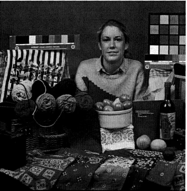
2.1 Picture Girl". Original ... 26
2.2 Bandwidth of FM signal (95% ). Picture "Girl" ... ... 27
2.3 Bandwidth of FM signal (95%). Sine wave message. . ... 28
2.4 Simple model of an FM transmission system . ... 29
2.5 Signal-to-noise ratio versus normalized carrier-to-noise ratio ... 32
2.6 Bandwidth-noise exchange function for two signals sources ... 33
2.7 The function g(x). .37 2.8 The masking function for the picture "Girl" . ... 40
2.9 Illustration of masking and noise perception . ... 42
3.1 Decomposition of the picture into Lows and Highs components ... . 44
3.2 Lows-Highs decomposition of "Girl" . ... 45
3.3 FM system for a sampled signal ... . . 46
3.4 Transmission parameters as a function of rolloff . ... 48
3.5 Block diagram of adaptive frequency system . ... 51
3.6 Evolution of the short-time bandwidth ... 53
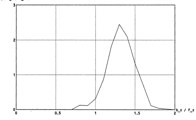
3.7 Histogram of the short-time bandwidth . ... 55
3.8 Original segment of "Girl" ... 56
3.9 Segment of "Girl" after adaptive frequency modulation transmission . 57 3.10 Segment of "Girl" after fixed deviation FM transmission ... 58
3.11 Probability distribution of the standard deviation in a block ... 59
3.12 Average masking improvement for a separable Gauss Markov process 62 4.1 Illustration of envelope distortion and bandlimiting distortion ... . 70
4.2 Effect of linear distortion on the Highs component ... 72
4.3 Effect of linear distortion on the four-by-four subbands issued from the Highs component ... 73
4.4 Third-harmonic distortion ratio of a first-order Butterworth filter for sinewaves at two different frequencies ... 75
4.5 Peak bandlimiting distortion for a bandlimited impulse ... 77
4.6 Minimum of envelope for a bandlimited impulse ... 79
4.7 Effect of envelope drop on click occurrence ... 81
4.8 Peak distortion measured for the preemphasized luminance signal. .. 84
4.9 Peak distortion measured for the Highs component. ... 85
4.10 Peak distortion measured for the subband -0-3. . . . .... 86
4.11 Peak distortion measured for the subband -3-0. ... 87 7
4.12 Peak distortion measured for the subband -3-3 .88 ...
4.13 Peak distortion measured for a white noise field . ... 89
4.14 Original picture cman" ... 91
4.15 Comparison of two algorithms ... 92
4.16 Iterative system for the update of the deviation function ... 93
4.17 Flow-chart of update computation ... 94
4.18 Bandlimiting distortion for many blocks as the deviation is increased. 96 4.19 Illustration of iterative algorithm ... . 98
4.20 Histogram of peak bandlimiting distortion on third iteration ... 99
4.21 Coded sequence with the PEFD algorithm . . . ... 101
4.22 Coded sequence with the frame-iterative algorithm ... 102
5.1 Coding gain due to preemphasis ... 107
5.2 Decomposition of the sequence into components ... 109
5.3 Coding gain due to subband decomposition ... 112
5.4 Sequential transmission of the components with variable rate. .... 113
5.5 Coding gain due to multirate FM ... . 116
5.6 Vertical decomposition of the picture "Girl" ... 118
5.7 Multirate FM coding of "Girl" . . . ... 119
5.8 Regular FM coding of "Girl" ... 120
5.9 Groups of subbands with common frequency deviation ... 124
6.1 Undecoded field of a MAC system ... . 128
6.2 Effect of noisy transmission of the side information. ... 133
6.3 Undecoded field of an adaptive MAC system ... 135
6.4 Segment of decoded frame of the adaptive MAC system ... 136
6.5 Components of HDTV system ... 140
6.6 Segment of a decoded frame of the HDTV system ... 144
8
List of Tables
3.1 SNR of different FM systems for "Girl" ... 61
3.2 SNR of adaptive FM system for "Girl" ... 63
4.1 Click occurrence for different CNR ... 80
4.2 Comparison of three algorithms ... 99
5.1 Multirate system for "Girl", vertical decomposition ... 117
6.1 Downsampling factors of the analog components and block size of the adaptation factors in a field of adaptive MAC . ... 130
6.2 FM transmission of side information . ... 132
6.3 Multirate specification of adaptive MAC system ... 134
6.4 Measurement of the decoded SNR in a frame of the adaptive MAC system ... 135
6.5 Downsampling factors of the analog components and block size of the adaptation factors in a frame of HDTV system . ... 139
6.6 Multirate specification of HDTV system . ... 142
6.7 Measurement of the decoded SNR in a frame of the HDTV system .. 142
9
I·----t
10
a*
--Acknowledgments
I wish to express my sincere gratitude to Professor Schreiber for his guidance, support, and encouragement. I am also grateful to my thesis readers, Prof. P. Humblet and Dr. A. Netravali, for their comments and suggestions. I want to thank all the members of the ATRP group for many interesting discussions and enjoyable moments.
Thanks also to my friends in Cambridge, New York, and Atlanta for very nice moments during my stay at M.I.T. In particular, Abeer was a great source of support, and also of fun. Her spirit and humor could not be replaced. Shukran. Thanks to Maurice and Philippe. The Swiss cheese fondue with Mont-sur-Rolle wine were certainly an essential ingredient in completing this thesis. I am also grateful to my family for their constant support and encouragement. Finally, I would like to thank Isabelle for her love and support.
This work has been supported in part by members of the Advanced Television Research Program, the Hasler Foundation, Switzerland, the Swiss National Fund for Research, and by the Brown Bovery Corporation, Switzerland.
11
12
To my parents
13
___~_ _· X1I_^--l~ _-1_L- _~ll_~l ~- LTIIII-LYI- I C~Y-· -r---ll
14
__ L*
Ah
Chapter 1
Introduction
Since the National Television Systems Committee adopted the present television stan-dard in 1953, no other coding scheme has been as widely used on the American con-tinent. However, this decade is witnessing a surge of research activity in the field, due largely to the advances of the Japanese high definition television systems and its European and American reactions.
In this changing landscape, satellites are very likely to remain important for dis-tributing and broadcasting television signals., Direct Broadcasting by Satellite (DBS) for example was recently introduced in Europe. Distribution by satellites of NTSC signals, on the other hand, is of great importance now, even for cable companies. The excitement produced by the coming of High Definition Television is motivating studies on how to do a better job in today's satellite systems and design new satellite systems for tomorrow's television.
Even though the trend in communication is to use digital transmission, frequency modulation, an analog modulation scheme, is often preferred for video satellite
appli-cations [Gag87].
Digital transmission involves source coding and channel coding. Source coding has the ability to remove most of the redundancy of the video signal, thus reducing the amount of information to be transmitted [JN84] [Ber71]. Channel coding is then required to map this digital information into signals suitable for transmission [Pro83].
15
However, the channels offered by satellites usually have a very poor signal-to-noise ratio, and a large number of error correction bits must be added in order to communicate reliably [Ga68], thus partially defeating the purpose of source coding
[MMHY87].
Frequency modulation, on the other hand, is quite adequate for video applications [Rho85]. Like digital coding, it has the ability to exchange bandwidth with distortion, but its distortion very nicely matches the human visual sensitivity making it much less annoying than quantization noise and other digital artifacts. Of course, the price one pays using analog modulation is the impossibility to regenerate the signal perfectly after transmission, a typical feature of digital coders. For broadcasting and distribution purposes, this is not a major problem as long as this noise is below the level of visibility. This is amply justified since only one unique transmission is going to occur between the transmitting station and the viewers homes.
The performances of a FM coder can be greatly improved by exploiting other properties of the human visual system such as noise masking or reduced chrominance resolution used so far only in digital coders. Reduction of as much as 25 dB of noise perception has been achieved by a digital coder using the masking effect [SB81]. Another form of digital data compression was achieved by relying on the frequency-dependent noise sensibility of the eye using subband coding and DPCM [W086].
Similar large improvements in the efficiency of analog channel utilization can be achieved by digitally assisting the frequency modulator without losing the advantages of analog communication.
Soft Versus Hard Threshold
Shannon showed that a reliable communication is possible if the channel noise is below a certain level [Gal68]. When the noise is increased above that, an abrupt change of performance occurs, and it is no longer possible to communicate.
This effect, called threshold effect, is also encountered in nonlinear modulation, such as frequency modulation, pulse width modulation, etc. In the case of FM
tele-16
vision systems, it is manifested by impulse-like degradations, called clicks.
.When digital coding is performed in a satellite channel, forward error correction is used. Block codes or convolutional codes add some redundant information that is used to correct the bits degraded by noise. However, as predicted by Shannon, the performance of these coders drops abruptly when the noise exceeds a certain level. As a consequence, the satellite link is most of the time excessively good, so as to withstand extreme situations such as heavy rains. The additional channel capacity is wasted most of the time, a costly thing to do in terms of the extra power required in the satellite, or the larger antennas required.
Contrastingly, frequency modulation has a softer threshold, in that performance is still satisfactory even when the noise level is above the threshold. As a matter of fact, most of today's programming that uses a satellite link -many do- are affected by clicks. This soft threshold is a big advantage in that the design of the budget link is facilitated, and that no capacity is wasted (up to a certain extent) to handle extreme noise level.
Technological Constraints
Introducing a new modulation method requires a careful evaluation of the existing system constraints such as spectrum division. Spectrum planning for satellites has resulted in a division of the total capacity into smaller bands of fixed bandwidths. These bands can be of 24 MHz, 27 MHz, or 36 MHz, depending on the application. Any new coding scheme will have to fit into this framework, either by transmitting more information, such as enhanced television, in one band, or by putting two or more video signals in one band, without sacrificing quality.
An example of the latter is a dual-in-one coder, a system where two video channels are inserted into one 36 MHz transponder [MMHY87]. However the resulting quality has been suitable only to News Gathering. The digital coder proposed is also very
complex.
17
1.1
Outline of the Thesis
The thesis consists of seven chapters, including the introduction and the conclud-ing remarks. They cover the different steps involved in the design of an adaptive modulation system.
Chapter 2 reviews some properties of frequency modulation. It is seen that the noise performance of the transmission link can be improved at the cost of an increased bandwidth. In order to examine this property in the context of image processing, a statistical model of pictures is presented. Finally, the effects of the human visual sys-tem are taken into account in order to define a subjective measure of the transmission noise.
Chapter 3 introduces adaptive frequency modulation as a technique to keep the short-time bandwidth of the modulated signal constant. In order to take into account the nonstationary nature of the picture, a more refined model is proposed, which uses the assumption of stationarity inside blocks of small dimensions. Based on this model, an algorithm to adjust the modulator is derived, and its performance is assessed experimentally. Finally, the subjective noise improvement is evaluated.
Chapter 4 refines the transmission link model in order to include the effects of bandwidth limitation on both the modulated and the demodulated signal. It appears that envelope distortion occurs on the modulated signal, and bandlimiting distortion occurs on the demodulated signal. It is then shown experimentally that consistent quality is possible when the short-time bandwidth is smaller than a fraction of the channel bandwidth. Based on this more complete model, improved algorithms to adjust the modulator are proposed.
Chapter 5 examines the problem of efficiently allocating the resource of the channel between different components of the visual information. In the context of subband decomposition, a sequential transmission of the subbands generates various amount of noise, and of various psychovisual importance, depending on the spatial frequencies of the component. It is shown that by adjusting the rate of transmission of each component, a better subjective balance is possible, yielding substantial improvement.
13
Finally, chapter 6 describes two-real world applications that demonstrate the po-tential of adaptive frequency modulation and multirate transmission.
19
20
---- 1
Chapter 2
Background
This chapter introduces the major aspects of frequency modulation. It is shown here that frequency modulation can exchange signal-to-noise ratio with bandwidth, and that this exchange depends on the statistics of the signal source. Elements of visual perception are introduced to define a more meaningful quality criterion.
2.1
Definitions
Frequency modulation can be most easily defined with the help of the complex phasor. A modulated signal z(t) is the real part of its complex phasor ,(t):
z(t) = Re(z(t)) (2.1)
Angle-modulated phasors have constant magnitude while their instantaneous phase +(t) varies with time.
z(t) = VAcei(t) j ' (2.2)
Frequency-modulated signals have the following instantaneous phase +(t):
(t) = 27rFt + 2rzvo y(r)dr (2.3)
where Fc is the carrier frequency, v is the gain of the modulator [Hz/V], and y(t) is the message to be transmitted. The instantaneous frequency Fi(t) , which is the
21
-derivative of the instantaneous phase, is in this case:
F,(t) = 1 d(t) FC + vy(t) (2.4)
2 dt
We see here that the instantaneous frequency varies in direct proportion with the signal.
The frequency deviation D is defined by:
D = vyo (2.5)
The value yo is a known quantity and thus specifying D is the same as specifying the modulator gain v. In the future, the modulator will be characterized by D instead of
V, and the value yo is assumed to be known. The reference value yo is usually taken as
the maximum value of y(t). In that case, D is the effective peak frequency deviation. When y(t) is modeled by a Gaussian random variable of mean my and variance
oy2, o is defined such that:
P(y(t) < Yo) = 0.99 (2.6)
or, equivalently:
yo = my + 2.5ay (2.7)
This definition, although a little arbitrary, introduces the useful notion of peak de-viation for a random message. In the future, we shall assume the signal y(t) to be zero-mean. If not, we can always assume that the mean value is transmitted before-hand and removed from y(t).
Finally, the modulation index is defined as:
D (2.8)
where F, is the maximum frequency of y(t) to be transmitted.
Signal Representations
In some instances we use a discrete representation of the video signal y(t), assuming a critical sampling at FN = 2F.. To stress the fact that a signal is discrete-time, the
square brackets are used. Hence the signal y(t) sampled at FN = 2F, is
y[n] = Y(t)It=nTN (2.9)
where TN = 1/FN.
In the following, F refers to the frequency variable of the Fourier transform, whereas f refers to the frequency variable of the discrete-time Fourier transform.
For raster-scanned signals with line duration H, the relation of the temporal signal
y(t) to its two-dimensional discrete representation y(i,j) is given by:
y(i,j) = y(iTN + jH) (2.10)
On other occasions, a three-dimensional discrete representation is used. In that
case:
y(i, j, k) = y(iTN + jH + kOH) (2.11)
where O is the number of lines per frame. Progressive scanning is assumed unless specified.
Context will tell what notation is used. The indexes i, j, k will always be used for horizontal, vertical, and temporal directions, respectively.
2.2
Bandwidth of FM Signals
The power spectrum Sz(F) of a stationary process z(t) is the Fourier transform of its autocorrelation function R,(r)[Pro83]:
R,(r) = E(z(t)z(t - r)) (2.12)
S.(F) = F(R(r)) (2.13)
There are many criteria used to define the bandwidth of a signal. Bandwidth can be defined on a percentage-of-energy basis using information on its power spectral density. Other possible definitions are the bandwidth necessary to pass the informa-tion with negligible distorinforma-tion, or the frequency separainforma-tion between carriers, so that negligible interference occurs.
23
The former definition is used in this chapter where it is defined as the band con-taining 95% of the power of z(t). Clearly this bandwidth depends on the signal y(t) to be transmitted -mostly its power spectrum density and its amplitude distribution-and on the modulator gain, or equivalently the frequency deviation D. A fixed de-viation D will yield different bandwidths for different pictures unless they are very similar. Thus the relation between bandwidth and modulation index characterizing an information source will be similar for pictures having similar statistics.
The assumption here is that a picture can be modeled as a stationary process. This model allows us to characterize a source by its average behavior.
2.2.1
Modeling of the Luminance Signal
Television luminance signals can be modeled by stationary processes. A model of-ten used in the literature is the first order Gauss-Markov model. In that case, the spectrum is:
2
S,(F) = (2.14)
rFo 1 + F/F0
where F is the process bandwidth and a is the luminance power. In practice, however, the spectrum is limited to a frequency F,, beyond which the power density is negligible.
The autocorrelation function of the luminance signal is, by inverse Fourier trans-form:
Ry(r) = a2 exp(-For) (2.15)
It can be shown that for such a signal z(t) is also a stationary process [Pap83]. For large frequency (i.e. at the tail of the frequency distribution), S(F) is approximated by a Gaussian spectrum [Tre68].
1 A /2 -(F- F) 2 -(F +
S.(F) 2 /'cTt [exp( 2ov 2 ) + exp( + F) 2 (2.16)
2 vf [exv 2p 2 2
In order to contain 95 % of the power, the bandwidth is:
B, = 4vay = 4 D (2.17)
24 24
or, equivalently:
B= 4 Y (2.18)
F, yo
Hence, the ratio of modulated bandwidth to basebandwidth is linearly related with the modulation index. It can be noted that only second-order statistics is needed for
this evaluation.
Figure 2.2 shows the measured bandwidth required to transmit 95% of the energy as a function of the modulation index for the picture Girl", together with the value predicted by the stationary model. Here yo/oa = 2.5. The curve predicted by the model fits the measurements very well.
2.2.2
Sine Wave Test Signal
For the particular, though unlikely, case where y(t) is a sine wave at frequency F. , a closed form of S,(F) exists [Pan65] [AM83].
S.(F) = C J,2(/)((F-(Fc + kF.)) + 6(F + + (F + kF)) (2.19)
2 k=-oo
where Jk(x) is the kth Bessel function of the first order. In that case, the bandwidth necessary to pass 95% of the power is:
B = 2NF, (2.20)
where N is the smallest positive integer such that:
N
E J~2(p) > 0.95 (2.21)
k=-N
The bandwidth necessary to pass 95% of the power was also approximated by
Carson [JT37]:
B, = 2(F + D) (2.22)
or, equivalently:
B 2 +/ (2.23)
F.
This value is often used as a simple design rule in FM system. Carson's approxi-mation is displayed on figure 2.3 , together with the exact values. Here yo/ay = vI.
25
^-Figure 2.1: Picture "Girl". The size is 512 x 512.
26
Modulated bandwidth over signal maximun frequency
ation index
Figure 2.2: Bandwidth of FM signal (95% ). Picture "Girl".
2.3
Noise Analysis
In a first approximation, the effect of the transmission of the modulated signal z(t) is to introduce an additive noise component ntot(t) which can be assumed white and Gaussian over the bandwidth allocated to z(t) . The bandwidth allocated to z(t) will be referred to in the following as the I.F. bandwidth (intermediate frequency). I.F. filtering is performed to remove components of the received signal outside the I.F. bandwidth as shown on figure 2.4. It is assumed in this chapter that the I.F. fil-tering doesn't affect z(t), a valid assumption if the signal bandwidth is smaller than the I.F. bandwidth. The effects of the filtering on z(t) are investigated in chapter 4.
27
ModuLated bandwidth over 4 3 3I 1 0 n's approxim ... ... . ,~~~~P * ,~/I /! 0.4 Wtion / I I i ! signaL frequency 1.6 0.8 1.2
Figure 2.3: Bandwidth of FM signal (95% ). Sine wave message. The power spectrum density of the additive noise is:
S.,o, (F) = 2 (2.24)
We can further assume that the equivalent noise n(t) entering the demodulator after I.F. filtering is zero outside the I.F. bandwidth. By considering the I.F. filter an ideal band-pass filter for the purpose of noise evaluation, very little inaccuracy occurs. The filtered noise can then be modeled as a band-pass process, and, as such, can be expressed by its quadrature and in-phase components [dC84]:
n(t) = ntot(t) * hIF(t) (2.25) n(t) = nll(t) cos(27rFt) + n (t) sin(27rFct) (2.26) 28 I I I I I jl t ... ... --- : Carsc ... ... -- / / / / / / .... / / / / / / / / // I --... '
frequency demodulator
-ntot(t)
Figure 2.4: Simple model of an FM transmission system The power spectrum density of nl(t) and nll(t) is:
S 1(F) = S.(F) = NO ; IF < BIF (2.27)
0 ; otherwise
It is assumed that the magnitude of n(t) is small compared to the magnitude of
z(t). This weak-noise analysis avoids the case where the phasor jumps 27r radians
when the noise plus signal trajectory encircles the origin [JI65]. This effect -also
called the threshold effect- manifests itself by large spikes on the demodulated signal.
2.3.1
Ideal Discrimination
The frequency demodulator shown in figure 2.4 is modeled as an ideal discriminator. The input to the demodulator is '(t) ,the noise corrupted and filtered version of i(t). The ideal discriminator performs a Maximum-Likelihood estimation of the phasor angle +(t).
ML = actan Im((t)) + iZ'r (2.28)
The estimate y'(t) of the transmitted signal y(t) is:
y'(t) = 2r dtML(t) -- * hdemod(t) (2.29) where hdemod(t) is an ideal low-pass filter of bandwidth F. which removes the noise components outside the signal bandwidth. For a sinewave message, F is assumed
to be the maximum frequency of such a test signal. For the more realistic case of a Gaussian message, F, is the bandwidth of the video signal required to ensure proper image quality. The message y(t) is also bandlimited to F. prior to transmission. The value of i in the right-most term in equation (2.28) is chosen to guarantee that no impulse occurs when the phasor crosses Xr and that the mean value of y'(t) matches that of y(t).
The error e,(t) due to transmission noise is the difference between the original signal and its estimate.
e,(t) = y(t) - y'(t) (2.30)
Using the weak-noise assumption, we can approximate the phase error and then the estimation error.
e(t)= ( 2yrv dt 1 d (n±(t)) Ar * h·d d(t) (2.31) As nl(t) is a stationary Gaussian process, the estimation error is also stationary and Gaussian. The power spectrum density of e,(t) under the weak-noise approximation is:
S,,(F) = (2)1 (2F)2S (F) ; FI I <F (2.32)
0 ; otherwise
We note that the error term due to the noise has a spectrum proportional to the square of the frequency. This noise is usually termed "triangular" noise as its shape is triangular when displayed on a log-log scale, such as that of a spectrum analyzer.
Ideal filtering was preferred in our transmission model over Wiener filtering for
hdemod(t). A Wiener filter minimizes the expected error square [Pap83]. It was
pre-ferred to leave the signal unchanged (no attenuation) in the baseband so as to avoid any horizontal blurring of the picture.
2.3.2
Signal-to-Noise Ratio
In the previous section, we found a closed form for the estimation error. Here, an ex-pression for the signal-to-noise ratio is derived. To display the results in a meaningful form, some definitions are necessary. The carrier-to-noise ratio is usually defined in
30
the literature as the ratio of the carrier power to the RMS noise power contained in the intermediate frequency band.
A2/2
CNR= A/2 (2.33)
BIFNo
The normalized carrier-to-noise ratio CNRo is defined for a noise on twice the base bandwidth only:
A /2
CNR 2F N (2.34)
The expected value of the error square can be obtained by integrating the error spectrum over the signal baseband.
F.
E(e(t)2) = Sen(F)dF (2.35)
where, again, Fo is the maximum frequency of y(t) to be transmitted.
The expected value of the error squared can then be expressed after evaluat-ing (2.35):
2
E(e(t)2) = N 2 (2.36)
Finally, the signal-to-noise ratio can be expressed as:
SNR E((t)= 2) =- 6(-)232CNRo (2.37)
For the two sources, it is evaluated to:
SNR = 332CNRO ; sinewave message (2.38)
0.96j 2CNRo ; Gaussian message
We see here that for a given noise spectral density, the signal-to-noise ratio increases with the square of the modulation index / .
Figure 2.5 shows the theoretical prediction of the SNR together with the exper-imental results obtained by computer simulation for the picture "Girl" and for the sinewave signal. It can be 'noted that for very low carrier-to-noise ratio, the weak noise approximation no longer holds. For larger CNR , the model matches the mea-surements very well.
31
SNR dB]
3 6 9 12 15 18 21 24 27
ruDO rl
Figure 2.5: Signal-to-noise ratio versus normalized carrier-to-noise ratio. Weak noise approximation. Top: sinewave. Bottom: Gaussian message. The modulation index is 0.4 and the I.F. bandwidth is 4 Fs.
2.4
Noise-Bandwidth Exchange
We have seen in the previous sections that the cost of increasing the modulation index -or equivalently the frequency deviation- is an increase in bandwidth. On the other hand, this increase will yield significantly better noise figure.
Here a measure of how the noise figure relates to the bandwidth is obtained.
2.4.1
SNR Improvement
The normalized carrier-to-noise ratio CNRo can be better understood as the SNR of a reference amplitude modulation suppressed carrier system. It can be thought of as SNRIf given the noise conditions of the channel.
32
I_ _ _ __ ___ _ _
The SNR of an FM system was derived in equation (2.37). The improvement obtained with frequency modulation is:
392
0.9632
; sinewave message ; Gaussian message SNR improvement k 2 3 4Figure 2.6: Bandwidth-noise exchange function for two signals sources
Let's define the bandwidth expansion factor k as the ratio of modulated bandwidth to basebandwidth.
Bz
F, (2.40)
where, again, B, is the 95% bandwidth, and F, is the bandwidth of hdemod(t) By using the approximations of equations (2.17) and (2.22), we can express the SNR improvement as a function of k. SNRFM 3(k 1)2 CNRo 6k2 16 ; sinewave message ; Gaussian message 33 SNRFM CNRo (2.39) (2.41) __1 1____1___1__1111-Y ^1_.._1·11 1__1_ -_ _._I I 7 U
Figure 2.6 shows the SNR improvement versus the bandwidth expansion factor for a Gaussian message and the sine wave signal.
2.5
Perception and Noise Evaluation
The design of a coding scheme for transmission or storage usually involves minimizing an associated cost function. For example, a channel coder for digital information seeks to minimize the probability of error on a single digit [Pap83]. Equivalently, a K-L transform coder minimizes the mean error squared by transmitting only the coefficients of the Karhunen-Loeve transform with largest variance [Pra78].
The mean square error is not an adequate criterion for coding images, as it doesn't reflect well the perceived image quality. Defining a valid subjective measure of quality is a very complex task [Gir88]. However, oie can improve the simple-minded mean square error criterion by incorporating elements of perception in the definition. Two elements will be used here, noise weighting and noise masking.
It is not intended to use sophisticated models of vision. Rather, we seek to intro-duce tools to better describe the performances of a system. It is hoped that these tools will fit in a more general communication engineering frame while still describing the requirements of visual information processing. Specifically, we shall define and evaluate the weighting factor and the masking factor.
2.5.1
Noise Weighting
In this section, the weighting function of the human visual system is evaluated for normal viewing conditions. The autocorrelation of the noise is then computed, from which the weighted noise mean square can be derived.
The response of the human visual system to different stimuli at different spatial frequencies is not uniform. Similarly, the response to a secondary stimulus (error signal) associated with a main stimulus (image) very much depends on the frequency content of the secondary stimulus. For example, high-frequency interference is less annoying than low-frequency interference.
In order to simulate the weighting effect of a viewer, the CCIR Rep. 637-2 defines the following low pass function to measure the weighted noise of 525-line television signals [Rho85]:
We(F) = 1 + j2FT (2.42)
(1 + j2rFT2)(1 + j2rFT3)
where T1 = 2.56#s., T2 = 3.7ps., and T3 = 730ns. It is defined for normal television
viewing conditions.
An equivalent weighting network for discrete pictures is defined below.
From the previous continuous-time weighting network, we aim to deduce a discrete-time equivalent network. The NTSC luminance bandwidth, for which this recommen-dation was intended, is 4.2 MHz. A discrete representation of a picture is obtained by sampling at the critical sampling frequency FN = 8.4MHz. This maps the one-dimensional raster-scanned signal into a three-one-dimensional discrete signal. It should be noted that very often sampling is performed at a higher frequency. For example, in the CCIR recommendation 601, it is performed at four times the color subcarrier (14.24 MHz). Pictures obtained in this way are horizontally oversampled. Such is not the case of the picture used in the MIT computer facility. In the following, critical sampling is assumed.
From the frequency response prototype in continuous time, it is desired to design a discrete-time filter with approximately same response. Different methods have been tried, and the most satisfactory is the frequency sampling method. It amounts to specifiy the discrete-time Fourier transform of our desired filter to equal the corre-sponding response of the prototype filter at a number of discrete frequencies.
W(f)lf=FTN = W(F); F = 0, ±FN/N, ±2FN/N,..., FN/2 (2.43) where N is a large even number and W(f) is the discrete-time Fourier transform of
w[n].
w[n] = IDTFTN(W(f)) (2.44)
The weighting function can be used for horizontal or vertical weighting of a sam-pled picture with square pixels.
35
In the following, we shall use the separable approximation which allows us to express a function of space as a product of single-variable functions. For example, the two-dimensionnal weighting function is the product of horizontal and vertical weighting:
w(i,j) = w[i]w[j] (2.45)
In a similar manner, the two-dimensional correlation of the error signal can also be expressed in a separable form.
Re,(,j) = R.[i]RU[j] (2.46)
First the continuous-time autocorrelation of the noise is evaluated, and then that of its discrete representation is derived.
Using equation (2.32), we find the time autocorrelation of the noise:
F2
Ren(r) (2 2v)2CNRo g(2F,) (2.47)
where g(x) is the second derivative of -sinc(x) = -sin(rx)/(rx), as shown on figure 2.7.
g(x) = sin(rx)( 2 + cos(7rx)( 2) (2.48)
7rx 3
The expected value of the error squared can be obtained by evaluating Ren (O). The limit of g(x) as x goes to 0 is yields a result consistent with equation (2.35).
We see that g(x) is negative for x = ±1. It demonstrates that e,(r) is very likely to change sign from one sample to the next when critical sampling is performed, illustrating the high-frequency structure of the noise. This contrasts with the sinc(x) function, the normalized autocorrelation of an ideally low-pass white noise, which is zero for x = ±1.
When a two-dimensional discrete representation of the signal is used, the horizon-tal autocorrelation of the noise is:
F2 RP[i] = (2 CNR g(t)lt=iTN (2.49) 36) 2CNRo 36 ______ __
g(x)
-10
V
-8 -6 -4 -2 0 2 4 6 8 10
Figure 2.7: The function g(x).
By evaluating the normalized correlation g(x)/g(O), we notice that it never exceeds 1% for x > 100. For a raster-scanned display, this means that the noise correlation from a pixel at one line to the next line is approximately zero, i.e. there is nearly no noise correlation from one line to the next. Hence, we find the vertical correlation of the error signal from line n to n + j:
(2.50) F2
6CNRov2
where 6[n] is the unit sample sequence [OS75].
The mean-square error of the weighted noise e.(t) can now be evaluated from the autocorrelation Fourier transform.
No r1/2 1/2
E(en(ij) 2 ) = (2rV)2A2
]/
(2xf,)2I
W(f,) 2 df,J/2 1 W(fj) dfj (2.51)
where fi, and fj are frequency variables related to the indexes i, j respectively. 37 2~. 2-2--- --- .... 2 ,. . . ... ,. .~~~~~~~~~~~i---... ... ... ... ... 1111 -11-1 1^1_ IIIII
-Finally, the weighting factor is defined. It is the ratio of the perceived noise power to the noise power. It reflects the subjective attenuation due to the human visual system, and depends on the type of interference. Its evaluation gives:
E(e2(ij))
¢",, =
E(e(
j)) = (,i ,j = 0.014 (2.52) which is, expressed in decibels:101og((wi) = -10.4dB (2.53)
10log((,j) = -6.2dB (2.54)
where Cwi and j are the weighting factors in the horizontal and vertical directions, respectively. The perceived impairment is reduced significantly due to the high-frequency structure of the noise, mostly in its horizontal direction. This aspect of frequency modulation is one of the reasons for its popularity in television applications. However, it appears that frequency modulation doesn't perform as well in the vertical direction as it does in the horizontal one.
2.5.2
Noise Masking
Masking denotes the reduced sensitivity to a secondary stimulus (error signal) due to the presence of a large primary stimulus. This phenomenon is related to the saturation effect of the discharge pattern of sensitive cells in the retina. This can be noticed on noisy television signals: noise is mostly perceptible on large blank areas. Masking manifests itself mostly by hiding noise close to edges (luminance jumps) and in texture-like part of the picture. It has been used in image coding, both for DPCM [NP77], and PCM [SB81] coders. The reader is referred to [NP77] for a more complete overview of the bibliography.
A model is introduced here to quantify the masking effect. The main goal of this model is to provide us with an analytical tool to evaluate system performance.
The model assumes that the error signal at pixel (i, j) is attenuated by a masking function Ma(i,j) [Tom86].
enm(i,j) = e,.(i, j)M(i,j) (2.55)
38
where enm(i,j) is a discrete representation of the masked error signal at pixel (i,j). The attenuation Ma(i,j) is a function of the activity function A(i,j) [NP77]:
i+l j+k
A(i,j) =
Z
E a(nt)-(i)ll(/2(IrnmH 1m +$tI))
(2.56)n=i-I t=j-k
which is a local average of the slopes in the neighborhood of (i, j). a is taken here to
be 0.35 and k=l=2.
m = x(n,t) - x(n - 1,t) (2.57)
mnt = x(n,t) - x(n,t -1) (2.58)
The masking function is related to the activity function through the polynomial:
M(ij) = 1 + KA(i,j) (2.59)
where K=0.04. Figure 2.8 shows the masking function for the picture "Girl". Close to an edge, our model predicts a maximum attenuation of 20 dB of the perceived error signal.
The masked error is obviously no longer stationary. However, for a given picture, we can derive the sample mean of the masked error square:
1 M-1 N-1
(enm (i, j)2) - MN EZE em(ij) (2.60)
i=0 j=0
The masking factor is the ratio of the masked noise to noise mean square values. It reflects the subjective attenuation of the noise power due to masking. It depends on the statistics of the picture. For a specified part of the picture, it can be evaluated:
em = (i, j) 2 (2.61)
where the sample mean is computed on that part of the picture.
For a stationary error signal, the average masking factor can be estimated by:
1 M-1 N-1
(m" MN
M(ij)
2 (2.62)i=0 j=O
where M, respectively N, is the vertical, horizontal, size of the picture, or the region of interest.
39
--- -- --- :--
---- --- --! --:
--
:
Figure 2.8: The masking function for the picture "Girl". The masking is unity in white regions.
40
_II 1_1 I I 1_1
2.5.3
Perceived SNR
Image quality, as perceived by the viewer, is not reflected by the signal-to-noise ratio calculated over the entire picture, but, rather, by evaluating it on small parts of the picture. Viewers usually object to the worst part of the picture [Tom86].
Hence, when the statistics of noise, or of other form of distortion, varies over the picture, a segmented evaluation of the signal-to-noise ratio is preferred. The same applies to the evaluation of the masking factor, which then describes the reduction of noise sensitivity in the small area of the picture for which it was computed. Texture-like parts of the picture will benefit a lot from this effect, while blank areas obviously will not benefit from it at all.
The perceived SNR for a segment of picture is:
perceived SNR = (2.63)
where (m is computed on that part of the picture.
To illustrate this concept, an example is developed.
It is desired to transmit "Girl" over a channel presenting a normalized carrier-to-noise ratio CNRo of 15 dB, using frequency modulation. From different bandwidth considerations, the modulation index P is set to 0.5.
We find that the SNR after demodulation is 9 dB. Taking weighting into account, the perceived SNR is 25 dB.
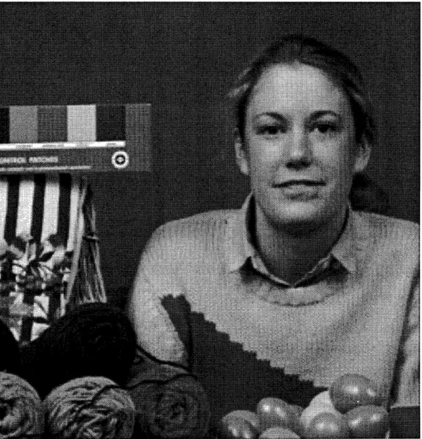
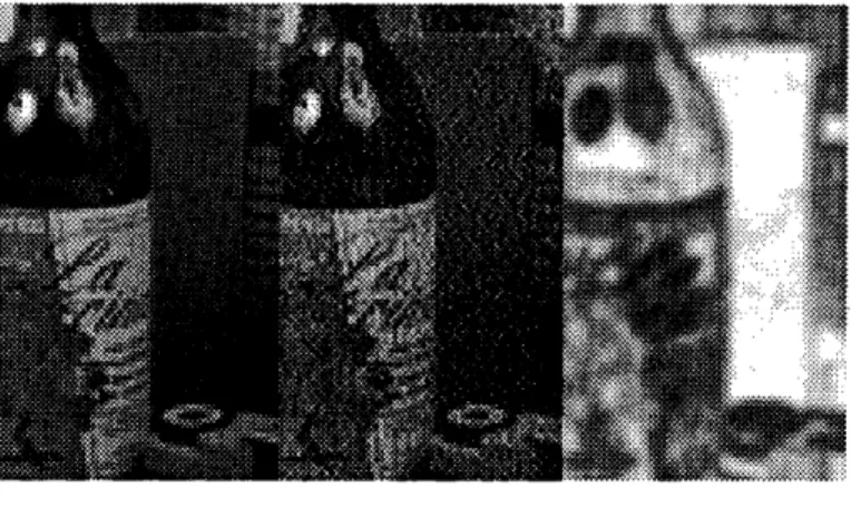
Next, we evaluate the factor due to masking. A small section of "Girl" is used for the purpose of demonstration, as illustrated in figure 2.9, where the masking function is shown next to the transmitted picture. The expected masking factor is 0 dB on the panel behind the bottle, whereas on the texture behind this panel it is about -7 dB.
On an edge, the factor is -14 dB (a conservative value). Finally, we find for the different areas:
25 dB ; panel
perceived SNR = 32 dB ; texture (2.64) 39 dB ; edge
41
Figure 2.9: Illustration of masking and noise perception. Left: original, middle: after transmission, right: masking function.
We can draw two conclusions from this example. First, some elements of perception, although very rudimentary, can help us to better evaluate a system performance. Second, it appears that frequency modulation doesn't perform uniformly over the picture, leaving room for improvement.
42
Chapter 3
Adaptive Frequency Modulation
In the previous chapter, we have evaluated the noise improvement for a given band-width increase. The information to be transmitted, a sequence of still pictures, was assumed to be stationary in the wide sense: the first- and second-order statistics do not vary over the picture [JI65]. It was also found that noise perception is not uniform across the picture.In this chapter, a scheme is presented to increase performance at little cost: an increased complexity of the encoder and decoder and the transmission of additional
side information.
3.1
Decomposition into Lows and Highs
The Gauss-Markov model of a raster scanned video signal is very approximate. The local mean of the luminance signal not only varies with scene content, but also it varies in different parts of the picture [HC76]. Similarly, a local measure of the variance ranges from zero on a uniform background to a large value in textures.
In order to match the Gaussian image model better, the local mean of the picture is removed. For the modulated signal, this amounts to reducing very-low-frequency variations of the carrier frequency. The local mean is obtained by low-pass filtering the picture.
The low-pass picture is downsampled by Ml x N1 in order to reduce significantly
43
this information, which will also be transmitted. The resulting component is called the Lows. An approximation of the low-pass picture is then obtained by interpolating the Lows up by the same factor. A component free of low-frequency variations, called the Highs, is computed by taking the difference of the original picture and its re-constructed low-pass version. Figure 3.1 shows how this decomposition is performed. The decomposition has proved to be fruitful for a digital coder [SB81]. Figure 3.2 shows the two components for "Girl", where Ml = N1= 4.
To compute the local mean, low-pass filtering is performed with a separable two-dimensional Gaussian prefilter.
h,.(i,j) = h.[i] h[j] (3.1)
where
1
22-h [i]= exp(- ) (3.2)
The standard deviation af of the filter impulse response is set to 1.6 when the down-sampling factor is 4 x 4 and to 3.2 when the downdown-sampling factor is 8 x 8. Recon-struction after downsampling is performed with a postfilter of same form, but with ao equal to 2.4, and 4.8, respectively. This class of filters is common in image processing
[ST85]. In this chapter a downsampling factor of 4 x 4 wil be used.
Lows
Figure 3.1: Decomposition of the picture into Lows and Highs components
44
(a)
(b)
Figure 3.2: Picture "Girl": (a) Lows component. (b) Highs component.
45
--3.2
Frequency Modulation of a Discrete Signal
A discrete representation of the signal is essential to perform operations such as com-ponent separation, as it permits the use of VLSI technology. Although the compo-nents defined above are discrete both in space and amplitude, the effect of amplitude quantization is ignored. Mathematical operation in the encoder and decoder can be performed with a sufficient precision so as to yield no noticeable alteration of the image.
In this section, the necessary mapping from a discrete signal to a continuous signal is reviewed, and the results are specialized to the FM case. Let's suppose that the encoder generates the samples of component I at a rate ri samples/sec. Let us assume that a channel is available with a bandwidth limited to B. We propose to find the performance of frequency modulation for such a discrete source.
Two additional blocks are needed to perform frequency modulation of a discrete signal. First, an interpolator maps the stream of samples xi[n] into a continuous signal y(t) which is fed to the modulator. Second, a combination of a matched filter and a sampler maps the continuous signal y'(t) obtained after transmission back into a digital stream xz[n]. This is shown in figure 3.3.
n_tot(t)
T x[
y(t) y'(t)
Figure 3.3: FM system for a sampled signal
Interpolation is performed with pulse pi(t):
y(t) = xir[n]p(t - nTj -
9)
(3.3)n
46
where T = l/ri. The initial phase 0 is a random variable uniformly distributed between 0 and r.
The pulse pt(t) used here has a raised-cosine spectrum [Pro83]. Other pulses are possible.
The receiving filter is matched to the transmitted pulse pi(t) and to the transmis-sion noise. To simplify the discustransmis-sion, we shall consider matching to a white noise. In this case, matched filtering amounts to specify the demodulator filter described in section 2.3.1 as having impulse response pl(t). A small gain would be possible by using a receiving filter matched to the triangular noise, or by using optimal joint pre-and postfilter [Mal86]. This is investigated in chapter 5.
hdemod(t) = pi(t) (3.4)
In our case, we have:
p,(t) *pi(t) = co- ( A sinc(rit) (3.5)
1- (4At)2
The pulse pi(t) convolved with itself satisfies the Nyquist criterion, which states that the Fourier transform of pt(t) * pt(t) must have a central symmetry around
F = r/2 to guarantee no intersymbol interference. The parameter A controls the
amount of roll-off. For A = 0, we are in the perfectly bandlimited case, as described in chapter 2. For larger A, the bandwidth of y(t) increases, but the trailing and leading oscillations of pl(t) decay more rapidly than for A = 0. This is an important feature to guarantee robustness when timing jitter is present in the receiver [Pro83]. In order to predict Bz, the bandwidth of the frequency-modulated signal, the second-order statistics of y(t) are needed. By modeling the discrete component I by a Gauss-Markov process with correlation coefficient pi, we define:
R
[n]
= oa p"n (3.6)Note that if the samples of xi[n] are transmitted in a random order, as is done in some scrambling schemes, the correlation coefficient is zero. The scrambled picture looks like white noise.
47
deltas 1.3 1. 1.1 0.5 1 1.3 1.2 (b) 1.1
1
rolloff V · 0 0.5 1Figure 3.4: (a) Standard-deviation ratio of interpolated signal y(t) to discrete signal
xl[n]. (b) Standard-deviation ratio of demodulated noise with roll-off A to
demodu-lated noise in the ideal bandlimited case. The spectral density of y(t) is:
S,(F) =
I
P(F)I 2 Uk - Pi )1 + p~ - 2p, cos(2irFT1
We find the ratio A2 of the variance of y(t) to the variance of
O,
1 j~+oo,12(1 - p2)
-2 =
= | P 1(F) j ~ 1 +p-2picos(2 A o , = +
- 2p(
cos(2, Figure 3.4 displays this ratio as a function of A. Hence, the bandwidth to half sample-rate is:k -= 4 '
r,/2 to
where x0 is a known quantity used to define D:
D = vxo
The modulation index P is defined, consistently with (2.8), as:
(3.7) zl[n]. FTL)df (3.8) ratio k of modulated) ratio k of modulated (3.9) (3.10) = D (3.11) ri/2
Equation (3.8) should be compared with (2.18). It can be shown that A, is always equal to unity. FM transmission of samples of a bandlimited process using inter-polation pi(t) requires the same bandwidth as if it were directly transmitted in a continuous form with the same peak frequency deviation.
48
(a)
rolt off o... .. .. . . ... . . . I ... ... --- -- -- ---delta n .I' n ·11 0 r I · ·The last block of figure 3.3 consists of a matched filter and a sampler. The sampling process is assumed ideal. We shall investigate the influence of pl(t) on noise performance.
The noise spectrum is:
Se(F) = (2rF)2SL(F) I P(F) 12 (3.12)
(2rv)2 A2
We find the expected error squared on xl[n]:
E(e[n]) = E((x[n] - x,[n])2) = E((y'(t)- y(t))2) =
I
Sn (F)dF = a6 Fn-,, 6 CNRIo v2 (3.13) The term A2 denotes the ratio of noise variance with rolloff parameter A to the noise variance in the ideal bandlimited case. Evaluation of equation (3.13) shows a modest increase of demodulated noise as the rolloff parameter A increases, as illustrated in figure 3.4.
Finally, the signal-to-noise ratio for a sampled source is:
SNR= E(x [n]) = 6 (al)2 32 CNRo (3.14)
E(e[n) a XO
where
A2/2
CNRo = 'N (3.15)
The SNR improvement is:
SNRFM 6k2
CNRo 162A2= (3.16)
When comparing (3.16) with (2.41), we see that the performance of a FM system for a sampled source is slightly inferior to that of the original continuous source. The change of performance depends on the rolloff parameter of the interpolation function. The receiver filter degrades the noise performance a little. In the following , the ideal interpolation pulse pl(t) with A = 0 is used, unless otherwise specified. In practical
applications, when timing jitter is a problem, the rollof A can be increased.
49
---3.3
Adaptive Modulation of the Highs
In the section 3.1, we transformed the luminance signal into a zero-mean discrete signal, called the Highs. The Lows component is transmitted separately as shown in chapter 6. However, we cannot assume that the statistics of the Highs are station-ary. A good approximation is to consider a picture as made of many small blocks inside which the statistics can be assumed constant. Every block is modeled by a multivariate Gaussian model whose parameters can be evaluated.
If the statistics of all blocks are known prior to transmission, it is possible to improve the performance of our modulalion cheme by adjusting the modulation index from block to block. The index in each block is transmitted to the receiver. By doing so, we must however respect a constraint on the usage of the channel. A logical constraint is to restrict the bandwidth of the modulated signal to be smaller than a preassigned value B, the channel bandwidth. More precisely, the short-time bandwidth b, where the bandwidth is estimated on a small period of time, must be limited. By using short-time bandwidth estimate, we can ensure that critical cases are handled equally well by a fixed bandwidth limited channel.
As noise performance improves for larger frequency deviation, the problem of optimum adaptive modulation can then be stated as follows:
* In block (m, n), choose the frequency deviation D(m, n) so as to: Maximize D(m,n) with constraint that the short-time bandwidth bz computed over the block region doesn't exceeds B more than 5 % of the time.
Varying the frequency deviation amounts to varying the modulator gain, as D is defined as the deviation for a given input yo. An optimal solution to this problem is very hard to treat analytically. It also depends on the algorithm and the window used for the short-time estimate. An approximate solution is developed here.
A block diagram of the adaptive frequency modulator is shown in figure 3.5. 50
---I---
-*-channel
I
I
n_tot(t)
Figure 3.5: Block diagram of adaptive frequency system
3.3.1
Derivation of the Deviation Function
In block (m, n) of size M times N, the standard deviation of a pixel in the block can be estimated:
1 (mM)+M-1 (nN)+N-1
&(m,n) = (MN
E
y(2j)2)2 (3.17)i=mM j=nN
In a window centered in the block (m, n) and for a given frequency deviation, a measure of the short-time bandwidth is obtained using equation (2.17), which states that the FM bandwidth is linearly related to the signal standard deviation for Gaus-sian processes.
Under the assumption that the Highs can be modeled by a Gaussian process, the deviation D(m, n) in block (m, n) yielding a short-time bandwidth equal to B is then:
D(m,n) = B (O (3.18)
where yo is a known constant, usually the peak value of y(t). In order to avoid abrupt change of noise performance from block to block, the deviation is varied smoothly using bilinear interpolation between block values. This avoids an artifact known as blocking effect. Because of occasional excessive bandwidth values, the index in (3.18)
51
is decreased by about 15% in practical cases.
D(m, n) = aB y (3.19)
4&(m, n) where ac = 0.86 for "Girl".
Alternatively, one can define a nominal deviation Do based on a specified stan-dard deviation a:
Do = aB Yo (3.20)
4cxrB
Then,
D(m, n) = fo(m, n)Do (3.21)
where f(m, n) is the adaptation factor for the block (m, n).
fa(m,n) a(mn) (3.22)
The adaptation factors comprises the extra information necessary to control the re-ceiver.
In order to verify that the short-time bandwidth is effectively linearly related to a local measure of the standard deviation, an experiment is performed. It compares what the Gaussian model predicts and what we measure.
Bandwidth measurement relies on spectrum estimation techniques. Power spec-trum estimates are affected by uncertainty and also bias. Specifically, a smoothing of the spectrum is obtained by windowing the estimated correlation function. The choice of the window will determine the trade-off between variance and bias of the power estimate. The popular Hanning window was selected for this application.
Another important effect of windowing is that a smaller window decreases the frequency resolution of the spectrum, a result well-known as the uncertainty principle
[dC84].
Figure 3.6 shows a typical scanned line of the Highs component y[i]. It is quite apparent here that the signal statistics vary a lot over the picture width. The mea-sured short-time bandwidth of the modulated signal z(t) is displayed below. Every block n is aligned with the corresponding segment of y[i].
52

![Figure 3.4: (a) Standard-deviation ratio of interpolated signal y(t) to discrete signal xl[n]](https://thumb-eu.123doks.com/thumbv2/123doknet/13860075.445428/48.915.83.800.118.349/figure-standard-deviation-ratio-interpolated-signal-discrete-signal.webp)