Terrain surfaces and 3-D landcover classification from small footprint full-waveform lidar data: application to badlands

HAL Id: hal-00460965

https://hal.archives-ouvertes.fr/hal-00460965

Submitted on 3 Mar 2010

HAL is a multi-disciplinary open access

archive for the deposit and dissemination of

sci-entific research documents, whether they are

pub-lished or not. The documents may come from

teaching and research institutions in France or

abroad, or from public or private research centers.

L’archive ouverte pluridisciplinaire HAL, est

destinée au dépôt et à la diffusion de documents

scientifiques de niveau recherche, publiés ou non,

émanant des établissements d’enseignement et de

recherche français ou étrangers, des laboratoires

publics ou privés.

small footprint full-waveform lidar data: application to

badlands

Frédéric Bretar, A. Chauve, Jean-Stéphane Bailly, C. Mallet, A. Jacome

To cite this version:

Frédéric Bretar, A. Chauve, Jean-Stéphane Bailly, C. Mallet, A. Jacome. Terrain surfaces and

3-D landcover classification from small footprint full-waveform lidar data: application to badlands.

Hydrology and Earth System Sciences Discussions, European Geosciences Union, 2009, p. 151 - p.

205. �hal-00460965�

www.hydrol-earth-syst-sci.net/13/1531/2009/ © Author(s) 2009. This work is distributed under the Creative Commons Attribution 3.0 License.

Earth System

Sciences

Terrain surfaces and 3-D landcover classification from small

footprint full-waveform lidar data: application to badlands

1_{Institut G´eographique National, Laboratoire MATIS, 4 Av. Pasteur 94165 Saint-Mand´e, France} 2_{Maison de la T´el´ed´etection, UMR TETIS AgroParisTech/CEMAGREF/CIRAD, 500 rue J.F Breton,}

34095 Montpellier, France

Received: 6 October 2008 – Published in Hydrol. Earth Syst. Sci. Discuss.: 6 January 2009 Revised: 13 July 2009 – Accepted: 28 July 2009 – Published: 26 August 2009

Abstract. This article presents the use of new remote

sens-ing data acquired from airborne full-waveform lidar systems for hydrological applications. Indeed, the knowledge of an accurate topography and a landcover classification is a prior knowledge for any hydrological and erosion model. Bad-lands tend to be the most significant areas of erosion in the world with the highest erosion rate values. Monitoring and predicting erosion within badland mountainous catch-ments is highly strategic due to the arising downstream con-sequences and the need for natural hazard mitigation engi-neering.

Additionally, beyond the elevation information, full-waveform lidar data are processed to extract the amplitude and the width of echoes. They are related to the target re-flectance and geometry. We will investigate the relevancy of using lidar-derived Digital Terrain Models (DTMs) and the potentiality of the amplitude and the width information for 3-D landcover classification. Considering the novelty and the complexity of such data, they are presented in details as well as guidelines to process them. The morphological val-idation of DTMs is then performed via the computation of hydrological indexes and photo-interpretation. Finally, a 3-D landcover classification is performed using a Support Vec-tor Machine classifier. The use of an ortho-rectified optical image in the classification process as well as full-waveform lidar data for hydrological purposes is finally discussed.

Correspondence to: F. Bretar

(frederic.bretar@ign.fr)

1 Introduction

Remote sensing aims at collecting physical data from the Earth surface. In this special context, these data are used as inputs in erosion/hydrological models or to monitor hydro-logical fields over large areas (Schultz and Engman, 2000; King et al., 2005).

Images obtained in the visible domain with passive op-tical sensors can be analysed for generating 2-D landcover and landform maps either automatically by image processing methods (Chowdhury et al., 2007) or by photo-interpretation. The use of the infrared channel helps to detect the vegetation (Lillesand and Kiefer, 1994). In a stereoscopic configura-tion, images are processed to generate Digital Surface Mod-els (DSMs) (Kasser and EgMod-els, 2002).

More recently, airborne lidar (LIght Detection And Rang-ing) systems (ALS) provide the topography as 3-D point clouds by the measurement of the time-of-flight of a short laser pulse once reflected on the Earth surface. Moreover, such active systems, called multiple echo lidar, allow to de-tect several return signals for a single laser shot. It is par-ticularly relevant in case of vegetation areas since a single lidar survey allows to acquire not only the canopy (the only visible layer from passive sensors in case of dense vegeta-tion), but also points inside the vegetation layer and on the ground underneath. Depending on the vegetation density, some of them are likely to belong to the terrain. After a clas-sification step in ground/off-ground points (also called filter-ing process), Digital Terrain Models (DTMs) can be gener-ated. Such DTMs are of high interest for geomorphologists to study erosion processes (McKean and Roering, 2004) or to map particular landforms (James et al., 2007). Moreover, hydrologic models such as TOPOG (O’Loughlin, 1986) or

TOPMODEL (Quinn et al., 1991) handle topographic data either as Digital Surface/Terrain Models or as meshes. By classifying terrain under different levels and types of vegeta-tion cover, lidar data could provide new land classificavegeta-tion, i.e., terrain, cover maps. This new 3-D landcover classifica-tion can be related to the hydrological processes that are usu-ally modelled in hydrological production indices as the SCS runoff curve number (USD, 1986), the runoff coefficient in the rational method (Pilgrim, 1987) or the plant cover fac-tor in Wischmeier and Smith’s Empirical Soil Loss Model (USLE) (Wischmeier et al., 1978). Lidar data have also been investigated by Bailly et al. (2008) and Murphy et al. (2008) for drainage network characterisation (Cobby et al., 2001; Antonarakis et al., 2008) and by Mason et al. (2003) as input data for flood prediction problems. For the latter, the au-thors use lidar data as resampled elevation grids and detect high and low vegetation areas. Vegetation heights are then converted into friction coefficients (Manning-Strickler coef-ficients) for hydraulic modeling.

Finally, multiple echo lidar data are typically used for the unique possibility of extracting terrain points as well as veg-etation heights with high accuracy. Hollaus et al. (2005) state the possibility to derive the roughness of the ground from li-dar point clouds. However, the filtering algorithm used to process lidar data is landscape dependent and the classifica-tion result may be altered (Sithole and Vosselman, 2004).

Based on the same technology as multiple echo lidar sys-tems, full-waveform systems record energy profiles as a func-tion of time. These profiles are processed to extract 3-D points (echoes) as well as other interesting features that could be related to landscape characteristics. Depending on the landscape properties (geometry, reflectance) and on the laser beam divergence angle (entailing small or large footprints), the recorded waveform becomes of complex shape. An ana-lytical modelling of the profiles provides the 3-D position of significant targets as well as the amplitude and the width of lidar echoes (Section 3.1). A detailed state-of-the-art of such systems can be found in Mallet and Bretar (2009).

This paper introduces a set of methodologies for process-ing full-waveform lidar data. These techniques are then ap-plied to a particular landscape, the badlands, but the method-ologies are designed to be applied to any other landscape.

Indeed, badlands tend to be among the most significant ar-eas of erosion in the world, mainly in semi-arid arar-eas and in sub-humid Mediterranean mountainous areas (Torri and Rodolfi, 2000). For the latter case, more active dynamics of erosion are observed (Regues and Gallart, 2004) with the highest erosion rate values in the world (Walling, 1988). Very high concentrations of sediment during floods, up to 1000 g l−1, were registered (Descroix and Mathys, 2003).

Badlands are actually defined as intensely dissected natu-ral and steeply landscapes where vegetation is sparse (Bryan and Yair, 1982). They are characterised by V-shape gullies that are highly susceptible to weathering and erosion (An-toine et al., 1995). These landscapes result from

unconsol-idated sediments or poorly consolunconsol-idated bedrock, as marls, under various climatic conditions governing bedrock disinte-gration through chemical, thermal or rainfall effects (Nadal-Romero et al., 2007).

The hydrological consequences of erosion processes on this type of landscapes are a major issue for economics, industry and environment: high solid transport, bringing heavily loaded downstream flood, are silting up reservoirs (Cravero and Guichon, 1989) and downstream river aquatic habitats (Edwards, 1969). Therefore, monitoring and pre-dicting erosion within badland mountainous catchments is highly strategic due to the arising downstream consequences and the need for natural hazard mitigation engineering (Mathys et al., 2003). Traditionally, the monitoring activi-ties in catchments are derived from heavy in situ equipments on outlets or from isolated and punctual observations within catchments. In complement to these traditional observations, hydrologists are expecting remote sensing to help them to upscale and/or downscale erosion processes and measure-ments in other catchmeasure-ments, by providing precise and con-tinuous spatial observations of erosion features or erosion driven factors (Puech, 2000). Among other inputs, erosion monitoring and modelling approaches on badlands (Mathys et al., 2003) need maps of landform features, mainly gul-lies (James et al., 2007) that are driving the way flows and maps of important driven factors of erosion in mountainous badland catchments. These factors are soil and rocks char-acteristics (Malet et al., 2003), vegetation strata used to de-rive 3-D landcover classes controlling rainfall erosivity, and the terrain topography (Zhang et al., 1996), which allow to derive slope and aspect of marly hillslopes (Mathys et al., 2003).

This paper aims to investigate the potential of using full-waveform lidar data as relevant elevation data, but also as a possible data source for 3-D landcover classification focus-ing on the characterisation of badland erosion features and terrain classification. If some papers have been published re-garding the interpretation of full-waveform lidar data, most of them are based on large footprint lidar data acquired from satellite platforms (Zwally et al., 2002). Very few researches have been carried out on the analysis of small footprint full-waveform airborne lidar data (Wagner et al., 2006; Jutzi and Stilla, 2006; Reitberger et al., 2008; Mallet and Bretar, 2009). Considering their novelty and their complexity, we propose to develop some new and specific guidelines related to their processing (including some physical corrections) and their management. Additionally, the extraction of the amplitude and the width of each echo is investigated as potential in-formation for landcover classification. Amplitude and width are related to the target reflectance as well as to the local ge-ometry (slope, 3-D distribution of the target). Finally, since colour images taken with an embedded digital camera are al-most always available at the same time as the lidar survey occurs, we investigated the use of additional colour informa-tion on the landcover classificainforma-tion results.

This paper begins with a background on full-waveform lidar systems (Sect. 2.1) as well as a brief presentation of a management system to handle the data (Sect. 2.2). We then present the processes to convert raw data into 3-D point clouds (Section 3.1). Sect. 3.2 is dedicated to the devel-opment of a filtering algorithm to classify the lidar point cloud into ground/off-ground points as well as on the gen-eration of DTMs. The echo amplitude and width extracted from full-waveform lidar data are described in Sect. 3.3. We focus this section on theoretical developments leading to a correction of amplitude values. Section 4 presents the badland area whereon investigations have been performed as well as the data: lidar data, orthoimages. DTMs pro-duced by our algorithm are then validated by the computa-tion of an hydrological index (Sect. 5) compared with man-ually (photo-interpretation) extracted ridges and valleys. We finally present in Sect. 6 the results of a 3-D landcover clas-sification using a vegetation class and different classes of ter-rain. This classification is based on a supervised classifier: the Support Vector Machines (SVMs). Different features have been tested, including the three visible channels of two orthoimages: the first one has been acquired with an embed-ded digital camera during the lidar survey, the second one is an extracted part of French national orthoimage database. The opportunity of using full-waveform lidar data for hydro-logical purposes is then discussed.

2 Managing full-waveform lidar data

2.1 Background on full-waveform lidar systems

The physical principle of ALS consists in the emission of short laser pulses, with a width of 5-10 ns at Full-Width-at-Half-Maximum (FWHM), from an airborne platform with a high temporal repetition rate of up to 200 kHz. They pro-vide a high point density and an accurate elevation descrip-tion within each laser diffracdescrip-tion beam. The two way run-time to the Earth surface and back to the sensor is measured. Then, the range from the lidar system to the illuminated sur-face is recorded (Baltsavias, 1999) as well as the trajectory of the plane. A lidar survey is composed of several parallel and overlapping strips (100 m to 1000 m width).

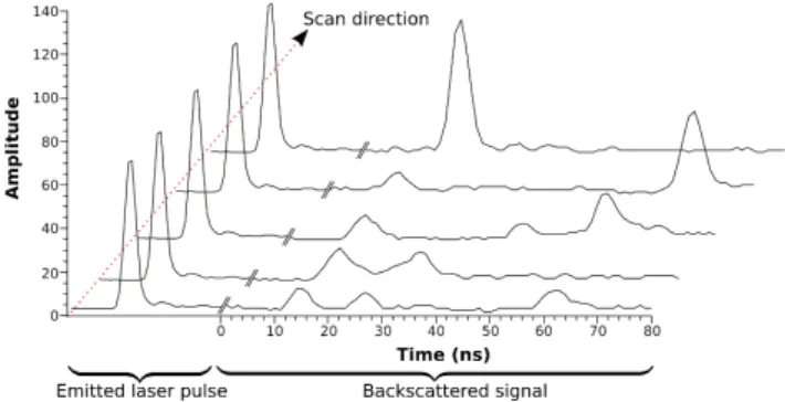
The emitted electromagnetic wave interacts with artificial or natural objects depending on its wavelength and is mod-ified accordingly. For ALS systems, near infra-red sensors are used (typical wavelengths from 0.8 to 1.55 µm). The se-lected Pulse Repetition Frequency (PRF) depends on the ac-quisition mode and on the flying altitude. Contrary to multi-ple echo systems which record only some high energy peaks in real time, full-waveform lidar systems record the entire signal of the backscattered laser pulse. Figure 1 shows raw full-waveform data.

Full-waveform systems sample the received waveform of the backscattered pulse at a frequency of 1 GHz. The

foot-Fig. 1. Raw full-waveform lidar data: five emitted pulses and their

respective backscattered signals.

print size depends on the beam divergence and on the fly-ing altitude. Most commercial airborne systems have a small footprint (typically 0.3 to 1 m diameter at 1000 m altitude).

2.2 Handling full-waveform lidar data

Initially, raw full-waveform lidar data are sets of range pro-files of various lengths. Raw propro-files are acquired and stored following both the scan angle of the lidar system and a chronological order along the flight track. After the georef-erencing process and the pre-processing step (Sect. 3.1), raw profiles become vectors of attributes containing, for each 3-D point, the x,y,z-coordinates, additional parameters (ampli-tude and FWHM) and a time-stamp that links it to the sen-sor geometry. Managing these data is much more complex than images: the topology (neighborhood system, topologi-cal queries) is designed to be as efficient as possible when accessing and storing the data. Indeed, the data volume is drastically larger than traditional laser scanning techniques: it takes 140 GB for an acquisition time of 1.6 h with a PRF of 50 kHz. Moreover, a 3-D/2-D visualisation tool is also nec-essary to handle the attributes, both in the sensor and in the ortho-rectified geometries. A specific software has therefore been developed for these purposes (Chauve et al., 2009).

3 Processing of full-waveform lidar data 3.1 From 1-D signals to 3-D point clouds

Contrary to multiple echo lidar sensors which provide di-rectly 3-D point clouds, full-waveform sensors acquire 1D depth profiles along the line of sight for each laser shot. The derivation of 3-D points from these signals is composed of two steps:

– The waveform processing step provides the signal

max-ima location, i.e., the range values, as well as additional parameters describing the echo shape.

– The georeferencing process turns the range value to a

{x, y, z} triplet within a given geographic datum.

WAVEFORM PROCESSING:

It aims at maximising the detection rate of relevant peaks within the signal in order to foster information extraction. In the literature, a parametric approach is generally chosen to fit the waveform (Mallet and Bretar, 2009). Parameters of a mathematical model are estimated. The objective is twofold. A parametric decomposition gives the signal maxima, i.e., the range values of the different targets hit by the laser beam. Then, the best fit to the waveform is chosen among a class of functions. This allows to introduce new parameters for each echo and to extract additional information about the target shape and its reflectance.

Our methodology is based on Chauve et al. (2007). The au-thors describe an iterative waveform processing using a Non-Linear Least Squares fitting algorithm. After an initial coarse peak detection, missing peaks are found in the residuals of the difference between the modelled and initial signals. If new peaks are detected, the fit is performed again. This process is repeated until no further improvement is possi-ble. This enhanced peak detection method is useful to model complex waveforms with overlapping echoes and also to ex-tract weak echoes.

The Gaussian function has been shown to be suitable to model echoes within the waveforms (Wagner et al., 2006). Its analytical expression is:

fG(x)= A exp −|x − µ|

2

2σ2

!

(1) where µ is the maximum location, A the peak amplitude, and

σthe peak width.

For each recorded waveform, the transmitted pulse is also digitised. By retrieving its maximum location, the time inter-val between the pulse emission and its impact on a target is known. The range value of the target ensues from the time-of-flight calculation.

The standard deviation σ corresponds to the half width of the peak at about 60% of the full height. In some applica-tions, however, the Full-Width-at-Half-Maximum (FWHM) is often used instead. We have FWHM = 2σ√2 ln 2.

GEOREFERENCING:

Similarly to multiple echo lidar sensors, computing the {x, y, z} coordinates of each echo in a geodetic reference frame from the range value requires additional data. The scan angle is used jointly to the range to calculate the {x, y, z} position for each point in the scanner coordinate frame. Then, the use of the GPS position of the aircraft, and the sensor attitude values (roll, pitch, heading) generate for each laser shot the

{x, y, z} in a given geodetic datum. Finally, the positions

can be transformed in some cartographic projection (French NTF Lambert II ´Etendu in this paper, see Section 4 for more details).

The transformation formulas cannot be expressed since they differ from one sensor to another. Offset values are dif-ferent, depending on the configuration of the laser system, GPS and Inertial Measurement Unit (IMU) devices.

After applying the advanced step of waveform modelling, full-waveform lidar data generate denser point clouds than multiple echo data. It is particularly relevant when studying the vegetation structure (Mallet and Bretar, 2009).

3.2 From point clouds to DTM

Basic processing of a lidar point cloud is the classification as ground/off-ground points, which is generally associated to the resampling of the data on a regular grid. Due to the accurate geometry of a lidar point cloud, many algorithms have been developed to automatically separate ground points from off-ground points (Sithole and Vosselman, 2004). Most of these approaches have good results when the topography is regular, but remain unperfect in case of mixed landscapes and steep slope conditions: parameters of the algorithms are often difficult to tune and do not fit over a large area. When ground points are mis-classified as off-ground points, the ac-curacy of the DTM may decrease (it depends on the spatial resolution and on the interpolation method). Inversely, when off-ground points (vegetation or man-made objects) are con-sidered as ground points, the DTM becomes erroneous which can bias hydrological models. Vegetated landscapes with sparse vegetation in a mountainous area (alpine landscape) are particularly interesting for the study of natural hydrology and the phenomenons of erosion (cf. Section 4). Neverthe-less, the processing of such landscapes need strong human interactions to correct the classification: since the detection of off-ground points of most algorithms are based on the de-tection of local slope changes, it may occur that the terrain (e.g., mountain ridges) shares the same properties. The DTM can therefore be over or under-estimated on certain areas de-pending on the algorithm constaints.

A methodology that handles these problems has been re-cently developed (Bretar and Chehata, 2008) and is used in this study to compute the DTMs. It is based on a two step process:

i. The computation of an initial surface using a predic-tive Kalman filter: it aims at providing a robust surface containing low spatial frequencies of the terrain (main slopes). The algorithm consists in combining a mea-surement of the terrain by analysing the elevation dis-tribution of the point cloud of a local area in the local slope frame (points of the first elevation mode – lowest points – belong to the terrain) and an estimation of the terrain height calculated from the neighboring pixels. The predictive Kalman framework provides not only a robust terrain surface (the slopes are also integrated in the predictive filter), but also an uncertainty σDTM for

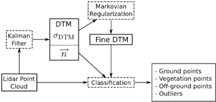
Fig. 2. Flowchart of the DTM generation from a lidar point cloud

associated to a classification pattern based on geometric rules.

ii. The refinement of this surface using a Markovian reg-ularisation: it aims at integrating micro reliefs (lidar points within the uncertainty σDTM) in a minimisation

process to refine the terrain description. Formulated in a Bayesian framework, additional prior information (ridge, valley etc.) can also be integrated in the refine-ment process.

The lidar point cloud is then classified based on geomet-ric criteria. A lidar point is labelled as GROUND if it is located within a buffer zone defined as the corresponding DTM uncertainty σDTM. Otherwise, it is considered asOFF -GROUND. In natural landscapes, off-ground points belong mainly to vegetation, and sometimes to human-made features (e.g., electric power lines, shelters). Vegetation areas are described as non-ordered point cloud (high variance) com-pared to human-made structures. Vegetation points are there-fore extracted by fitting a least-square plane within a circu-lar neighborhood centered sequentially on every off-ground points. If the residuals (average of orthogonal distances) are higher than a defined threshold (0.3 m), points are labeled as

VEGETATION. Figure 2 summarises the entire algorithm to calculate a DTM from a lidar point cloud. This classifica-tion is not explicitly used in the following, but for generat-ing the validation set related to the supervised classification (Sect. 6).

3.3 Processing the amplitude and the width of lidar echoes

Beyond the 3-D point cloud, full-waveform lidar data pro-vide the amplitude and the width of each echo (Sect. 3.1) that are potential relevant features for landcover classification. The backscattered amplitude (or received power) is a func-tion of the laser power, the distance from the source to the tar-get, the incidence angle, the target reflectivity, the absorption by the atmosphere. The use of such features in a landscape classification framework necessitates a global homogeneity between all strips (Wagner et al., 2008b; Kaasalainen et al., 2009). These features therefore need to be corrected from the above-cited contributions so as to be homogeneous and

thus, used in a landscape classification framework. We pro-pose also to analyse the effect of the incidence angle on the Full-Width-at-Half-Maximum.

3.3.1 The amplitude

Since the recorded amplitude is proportional to the backscat-terred flux and assuming the surfaces to be Lambertian, a fea-ture proportional to the target reflectance is derived from the recorded amplitude by applying the following corrections:

1. Incidence angle: Since the apparent reflecting surface is smaller in case of non-zero incidence angle than in case of zenithal measurements (a cosinus dependency), recorded amplitude values of bare ground points are corrected from the scalar product of the emitted laser direction by the corresponding terrain local slope ex-tracted from the DTM, which is cos θincidence,

2. Range correction: The recorded amplitudes are cor-rected by the ratioR2

R2 s

where R is the currrent range and

Rs a standard range (H¨ofle and Pfeifer, 2007),

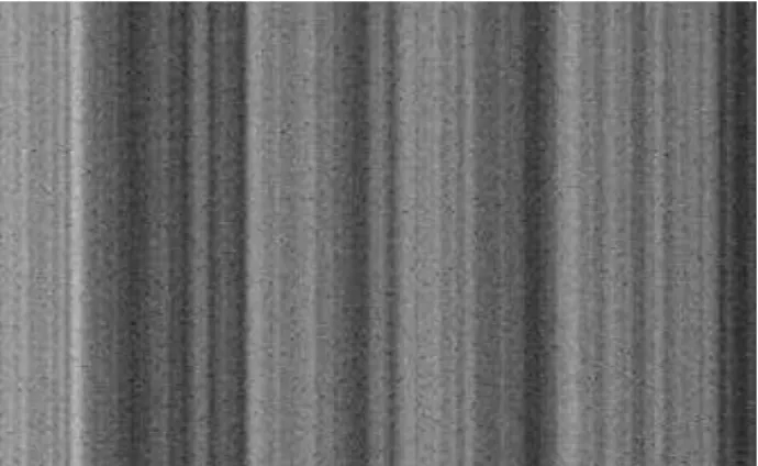
3. Emitted power: We have also remarked that the am-plitude of emitted pulses has high temporal variations which may be visible in the amplitude image and there-fore alter the spatial analysis of the data. Figure 3 rep-resents a small region of a laser band in the sensor ge-ometry, i.e. in which one pixel is linked toss one emit-ted pulse and one recorded backscattered signal. Fig-ure 3(a) represents the ratio between the amplitude of each emitted pulse and the average amplitude of all emitted pulses over the whole strip. The x-axis is along the flight track and the y-axis is along the scan direc-tion. Figure 3(a) shows high variations of the emitted power along the flight track, and similar variations (ver-tical lines) are visible on the image of first echo plitude (Fig. 3(b)). We therefore normalized the am-plitude of each measured peak (Ameasured) by the

ra-tio of the average amplitude value of all emitted pulses (Amean whole strip) and the amplitude of the emitted pulse

of the current peak Acurrent. The effects of the

correc-tion are presented in Fig. 3(c) where vertical lines have disappeared.

The whole correction procedure is described in Eq. (2) hereafter:

A = Ameasured cos θincidence

Amean whole strip

Acurrent R2 R2 s (2) 3.3.2 The Full-Width-at-Half-Maximum

The FWHM has shown some spatial variability in our data set. Considering the badland and alpine landscape, we inves-tigated the influence of the incidence angle on the FWHM

(a) Ratio between the amplitude value of the emitted laser pulse and the average amplitude values over the whole strip. Values are represented in grey level scale and stretched between 0.72 and 1.35

(b) Raw return amplitude of the first echo. Values are repre-sented in grey level scale and stretched between 0 and 150.

(c) Corrected return amplitude of the first echo from the laser fluc-tuations. Values are represented in grey level scale and stretched between 0 and 150.

Fig. 3. Effect of the correction from the laser fluctuations. Images

are presented in the sensor geometry.

only in case of bare soil areas. Indeed, the FWHM of under-vegetation ground points may have been modified by the complex optical medium. These investigations have been

performed on simulated waveforms reflected by a tilted pla-nar surface (Kirchhof et al., 2008). The simulation consists in a temporal convolution product between the emitted laser pulse chosen of Gaussian shape, the impulse response of the receiver, the spatial beam profile and the illuminated area.

We show that, for a divergence angle of 0.4 mrd, a flying altitude of 600 m, and an emitted Gaussian pulse of FWHM= 5 ns, the variations of the received pulses with regard to the emitted ones are respectively of 0.03 % (0.001 ns), 0.57 % (0.03 ns) and 5.3 % (0.26 ns) for an incidence angle of 10°, 30° and 60°. The effect of the in-cidence angle is therefore negligible on the pulse stretching with respect to the temporal sampling interval (1 ns).

We cannot extend this conclusion for ground points be-low the vegetation since the waveform has been modified through the canopy cover. The spatial variability is there-fore attributed to a more complex spatial beam response of the surface due to structures and/or reflectance properties.

4 Materials

Lidar data have been acquired over the Draix area, France. It is an experimental area on erosion processes in badlands located in the South of the French Alps. It belongs to the Euromediterranean Network of Experimental and Represen-tative Basins (ERB). The Draix area consists in five research experimental catchments, highly equipped and monitored for more than thirty years. Thirteen research units working on erosion and hydrology processes are grouped within the GIS Draix organisation (Mathys, 2004). Results for the most two eroded catchments are presented here: they concern the Laval and the Moulin catchments.

4.1 Lidar data

The data acquisition was performed in April 2007 by Sint´egra (Meylan, France) using a RIEGL© LMS-Q560 sys-tem. This sensor is a small footprint airborne laser scanner and its main technical characteristics are presented in Wagner et al. (2006). The lidar system operated at a PRF of 111 kHz. The flying altitude was approximatively 600 m leading to a footprint size of about 0.25 m. The point density was about 5 pts/m2.

The temporal sampling of the system is 1 ns. Each return waveform is made of one or two sequences of 80 samples. For each profile, a record of the emitted laser pulse is also provided.

4.2 Orthoimages

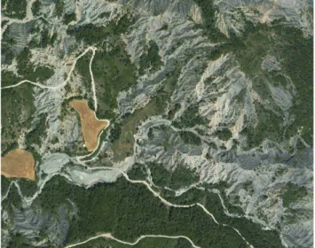
Two orthoimages were available for the study. The first one (Fig. 4(a)) is extracted from the French IGN data ba-sis BDOrtho©. Acquired in fairly good conditions (al-most no shadowed zones) by the IGN digital camera, a physical-based radiometric equalisation process has been

(a) Orthoimage extracted from the IGN BDOrtho© (RGBIGN).

(b) Orthoimage acquired during the lidar survey (RGBRAW)

Fig. 4. Two orthoimages showing RGB_RAWand RGB_IGNover the

Draix area.

applied (Paparoditis et al., 2006). The ground resolution is 0.5 m. The triplet of {red, green, blue} channels of the IGN image will be referred in this article to as RGBIGN. The

second orthoimage (Figure 4(b)) has been calculated from aerial images acquired during the lidar survey by an embed-ded digital camera (Applanix DSS Model 322). Since the survey has been performed early in the morning, numerous shadowed areas appear. Moreover, no radiometric equalisa-tion has been performed entailing a rather poor radiometric quality (see Figure 9). The ground resolution is 0.2 m. The triplet of {red, green, blue} channels of this image will be referred in this article to as RGBRAW.

5 DTM analysis with hydrological indices and photo-interpretation

The quality assessment of a DTM for hydrological purposes is not completely satisfying when considering only the ele-vation error distribution. Other DTM quality criteria directly connected to the usual hydrological information extracted from DTM may be used: drainage networks, drainage areas, slopes like presented in (Charleux-Demargne, 2001). These criteria are mainly based on the basic landform information related to the first and the second derivative of a DTM. How-ever, these criteria are not easy to use in a qualification pro-cess since (1) they are conditioned by both the algorithms

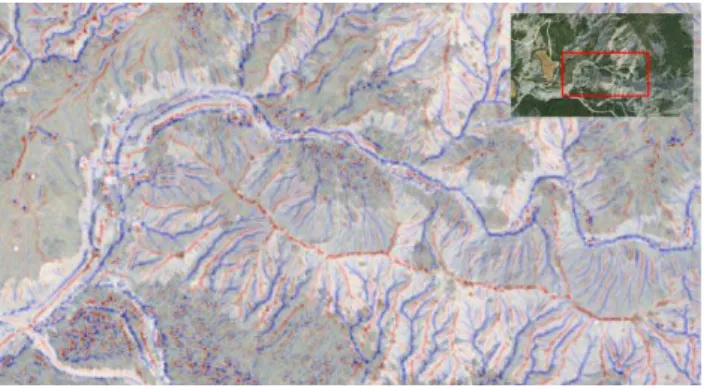
Fig. 5. CI computed on lidar data superimposed to the orthoimage.

and the parameters used to produce the information (e.g., a drainage area threshold in the D8 flow accumulation al-gorithm (O Callaghan and Mark, 1984)), (2) reference data are not easily available (how to survey drainage networks?) and finally (3) the quantification of quality is often not prop-erly defined (how to compare dissimilarities of drainage net-works?). Moreover, criteria are usually not generic: it is re-lated to a specific hydrological index.

In order to overcome these problems, a single criteria is proposed for a quantified auto-evaluation of DTMs at a given resolution in erosion areas with an hydrological and morpho-logical point of view.

This criteria is simply the linear part (in percentage) of ridges and valleys observed from an orthoimage that fall within areas having significantly non null convergence in-dex (CI) values computed on the DTM (K¨othe and Lehmeier, 1994). The convergence index corresponds, for each DTM cell, to the mean difference between angle deviations. These angle deviations are calculated in each of the eight adjacent pixels. For an adjacent pixel, the angle deviation is the ab-solute difference, in degrees, modulo 180, between its as-pect and the azimuth to the central pixel (Zevenbergen and Thorne, 1987). The convergence index is a symmetric and continuous index ranging from −90° up to 90°. This in-dex highlights ridges when highly positive and valleys when highly negative. Figure 5 shows the convergence indexes computed on the lidar strip. Main valleys and ridges appear with respectively highly negative (blue) and positive (red) values.

At a given location, a valley (resp. a ridge) is considered to be detected in the DTM if CI values belong to [−90°, −η] (resp. to [η, 90°], η ∈ R). On a DTM representing inclined planes without noise, only CI=0 (i.e., η=0) indicates the ab-sence of ridges and valleys, whatever the slope is. When dealing with noisy DTM, thresholding the CI with η to re-trieve significant ridges and valleys becomes a challenging task. We therefore simulated a distribution of CI from a set of 1000 virtual noisy DTMs. They were generated with a trend corresponding to a plane of constant slope (e.g., 33° is the

(a) (b)

Fig. 6. _{(a) Test area (85×85 m) with photo-interpreted valleys}

(blue) and ridges (red). (b) Detection of significant ridges (red) and valleys (blue).

mean slope of Draix area). The simulation consists in gen-erating Gaussian random fields (Lantuejoul, 2002) using the LU method (Journel and Huijbregts, 1978) following noise spatial distribution models with parameters: range, nugget and sill (variance) for spatial covariance.

Since the simulated CI distribution is of Gaussian shape, we set η to two times the standard deviation. We accept that five percents of CI values due to hazard on noise can be clas-sified in significant ridge and valley.

We show some results on a sub-area of Draix. The simu-lated CI distribution (performed on 33° slope, Gaussian noise of zero mean and 2.66 standard deviation) provides a thresh-old value η = 8.46. We show the results of the valley and ridge detection on Fig. 6.

Figure 6(a) is a manual delineation of apparent ridges and valleys. The photo-interpretation process is applied on main structures, but very close linear elements as well as the ele-ments near sporadic vegetated eleele-ments are not considered.

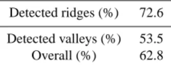
Table 1 presents the quality criteria obtained with the auto-matic approach (Figure 6(b)). The overall accuracy is 62.8%. This relatively low value can be explained by the following grounds. Firstly, the threshold η has been automatically cal-culated: the parameters of the simulation may be refined to reach better results. Secondly, the photo-interpreted valleys and ridges have been extracted from a 0.2 m-resolution image and then compared to a 1 m-resolution DTM: reliefs smaller than the resolution cell of the DTM are smoothed. Thirdly, if large ridges and valleys are well defined in the DTM, they may not appear in the photo-interpreted features since they may either be located in shadowed areas (valleys) or in sat-urated bright areas (ridges). The comparison is therefore bi-ased.

The observation of local erosion processes requires a more detailed relief restitution. Other techniques like terrestrial LiDAR or photogrammetry by unmanned aerial vehicles (Ja-come et al., 2008) are more accurate and precise, but, are not

Table 1. Morphological quality criteria results

Detected ridges (%) 72.6 Detected valleys (%) 53.5 Overall (%) 62.8

well adapted to survey large areas. However, considering the elevation accuracy of DTMs (approximately 0.9 m for 2 stan-dard deviation on the elevation random error), and that the lo-cal ablation speed over Draix area is of 1.5 cm per year (Oost-woud and Ergenzinger, 1998), change detection and monitor-ing of erosion effects would require a delay between surveys of several decades. Nevertheless, the loss of sediment vol-ume within catchments are not homogeneous and are tem-porary stored on hill-slope gully networks: 200tons/km2are trapped in the gully network, which corresponds to an ap-proximate of 150 m3(Mathys et al., 1996). These volumes are significant enough to shorter time lag for a multidate anal-ysis of DTM derived by full-waveform LiDAR (lower than a decade), even with an accuracy of some decimeters. Only full-waveform LiDAR survey which gives an adequate com-promise between precision, accuracy and extent makes pos-sible the monitoring of sediment volume displacement in the gully network at a catchments scale.

6 3-D landcover classification 6.1 Methodology

Lidar data have been used so far as accurate elevation data to extract ground points and generate DTMs. The challenges were to automatically process the data in a mountainous landscape with steep slopes and vegetation, the whole with the highest accuracy. We mentioned in the introduction that a landcover map is an important input of hydrological mod-els, especially for the parameterisation of the hydrological production function. We therefore propose in this section to describe the inputs and outputs of a classification framework wherein lidar width and amplitude values can be integrated and their benefit evaluated. Indeed, the interpretation of ad-ditional lidar parameters has been barely studied and reveals to be of interest for landcover classification. Wagner et al. (2008a) proposed classification rules based on a decision tree for vegetation/non-vegetation areas in a urban landscape us-ing solely the width and the amplitude: a point is consid-ered asVEGETATIONif (1) it is not the last pulse of a pro-file containing multiple returns (2) it is a single return with low amplitude (≤75) and large width (≥1.9 ns). Focusing on the study of the vegetation, Reitberger et al. (2008) have integrated different features to segment individual trees in a normalized graph-cut framework. Among them, the authors show that the feature corresponding to the average intensity

on the entire tree plays the most important role in leaf-on conditions, while the ratio between the number of single re-flections and the number of multiple rere-flections is the most important in leaf-off conditions.

Here, we would like to answer the question: do lidar width and intensity values improve a classification pattern in bad-lands? An efficient supervised classification algorithm called Support Vector Machines (SVM) has been used (Chang and Lin, 2001). In recent years, SVM was shown to be a rele-vant technique for remote sensing data analysis (Huang et al., 2002): ability to mix data from different sources, robust-ness to dimensionality, good generalisation ability and a non-linear decision function (contrary to decision trees for in-stance). In this paper, the 3-D lidar point cloud is labelled, thus providing a 3-D landcover classification. Mallet et al. (2008) applied this technique with success for classifying ur-ban areas from full-waveform lidar data.

Four classes have been identified focusing on a first and simple hierarchical level of 3-D land cover classification, rel-evant for badlands landscapes with anthropogenic elements: 1-LAND, 2-ROAD, 3-ROCKand 4-VEGETATION. The three first classes are increasingly sensitive to erosion processes. The first classLANDis taking into account terrain under nat-ural vegetation cover and cultivated areas in grassland. The second one,ROADs, are linear elements with natural (marls), bared but compacted material. These elements are known to impact runoff production within catchments. The third one contains areas with bared black marls in gullies, the main source of sediment production. The latter, vegetation, is a very general land cover class. This class is aggregating more detailed vegetation charcateritics, such as the 3-D vegetation structure, wich can be very usefull to dicriminate further.

The SVM algorithm requires a feature vector for each 3-D lidar point to be classified. Only three lidar features have been retained. Indeed, it appears that the larger the number of features, the more difficult to make an interpretation of the results. They are:

– dDTM, the distance between the 3-D point and the DTM,

– FWHM, the echo width (see Section 3.1). – Amp, the echo amplitude,

Additionally, RGBIGN or RGBRAW features have been

added in the classifier, providing three radiometric attributes (Fig. 8). Their introduction allows a discrimination between road and land impossible with the lidar features and improve the classification results. The training set over each of the four classes has been defined as follow:

– ROADandROCK: 200 lidar points are selected in a road and rock mask defined on the orthoimage.

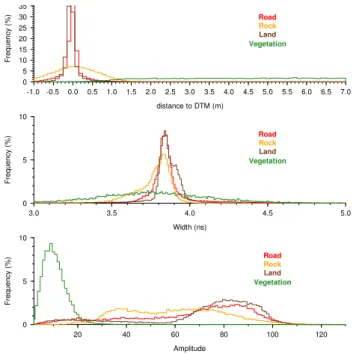
– VEGETATION: 200 lidar points are selected within a vegetation mask (lidar points classified as vegetation in Sect. 3.2) 0 5 10 F re q u e n cy (% ) 20 40 60 80 100 120 Amplitude Road Rock Land Vegetation 0 5 10 F re q u e n cy (% ) 3.0 3.5 4.0 4.5 5.0 Width (ns) Road Rock Land Vegetation 0 5 10 15 20 25 30 35 F re q u e n cy (% ) -1.0 -0.5 0.0 0.5 1.0 1.5 2.0 2.5 3.0 3.5 4.0 4.5 5.0 5.5 6.0 6.5 7.0 distance to DTM (m) Road Rock Land Vegetation

Fig. 7. Histograms of Amp, FWHM and dDTMfor the four classes

ROAD,ROCK,LANDandVEGETATION.

– LAND: 200 lidar points are selected (1) in a land mask on the orthoimage (2) in the intersection of the vegeta-tion mask and a ground mask (lidar points classified as ground in Sect. 3.2).

We have implemented the SVM algorithm with the LIB-SVM software (Hsu and Lin, 2001), selecting the generic Gaussian kernel. For more theoretical explanations, please see (Pontil and Verri, 1997).

6.2 Results

Figure 7 shows the histograms of lidar derived features cor-responding to the four selected classes. dDTMand Amp have

bounded values which describe the vegetation (resp. > 1 m and between 0 and 20), whereas the width values tend to be uniform between 3 ns and 4.5 ns.ROADandLANDhave sim-ilar distributions for lidar derived features, which explains the high confusion values in Table 2. The distributions of

ROCK is flattened for dDTM since many points are chosen

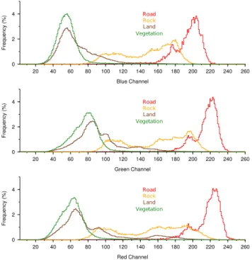
in very steep slopes, and are therefore more sensitive to the DTM quality. The amplitude of ROCK is slightly different from the other classes. Figures 8 and 9 show the histograms of RGBIGNand RGBRAW.

The classification is validated with lidar points belonging to the masks defined in the training step, but the training points. 40% of the total number of points have been vali-dated. Figure 10 shows the four validation sets for each class. A confusion matrix is then calculated for each configura-tion. True positive values correspond to the diagonal values

0 2 4 Frequency (%) 20 40 60 80 100 120 140 160 180 200 220 240 260 Red Channel Road Rock Land Vegetation 0 2 4 Frequency (%) 20 40 60 80 100 120 140 160 180 200 220 240 260 Green Channel Road Rock Land Vegetation 0 2 4 Frequency (%) 20 40 60 80 100 120 140 160 180 200 220 240 260 Blue Channel Road Rock Land Vegetation

Fig. 8. Histograms of RGBIGNfor the four classesROAD,ROCK,

LANDandVEGETATION.

0 2 4 Frequency (%) 20 40 60 80 100 120 140 160 180 200 220 240 Red Channel Road Rock Land Vegetation 0 2 4 Frequency (%) 20 40 60 80 100 120 140 160 180 200 220 240 Green Channel Road Rock Land Vegetation 0 2 4 Frequency (%) 20 40 60 80 100 120 140 160 180 200 220 240 Blue Channel Road Rock Land Vegetation

Fig. 9. Histograms of RGB_RAWfor the four classesROAD,ROCK,

LANDandVEGETATION.

Fig. 10. Ground truth classification of lidar points for each class LAND (dark brown and green), ROAD (red), ROCK (orange) and

VEGETATION(dark green).

Table 2. Confusion matrix corresponding to the classification with

{Amp, FWHM, dDTM}.

# points ROCK ROAD VEGETº LAND

71 216 ROCK 69.6 22.4 0.4 7.3 13 244 ROAD 7.5 84.2 0.1 6.6 402 995 VEGETº 0.9 0 94.2 4.7 279 321 LAND 9.1 19.4 2.7 68.6

AA 79.1%

of the confusion matrix. The accuracy of the classification results are quantified by the average accuracy AA, mean of the diagonal values of the confusion matrix.

AAdoes not depend on the number of points in each vali-dation set.

When using solely lidar derived features {dDTM, Amp,

FWHM}, Table 2 indicates that the confusion between

classes is not negligible particularly for some of them:ROCK

withROADreaches 22.4%, whileLANDwithROADreaches 19.4%, what was predictable looking through the statistics of the training set (Fig. 7). The vegetation has a high percentage of true positive (94.2%) and is well detected. With an aver-age accuracy of 79.1%, it appears that a classification based only on lidar derived features is consistent.

Before testing the effects of lidar amplitude and com-bined width with RGB features, we investigated the impact of the radiometric quality of the orthoimages on the classi-fication results. Tables 3 and 4 are the confusion matrices corresponding to the classification results with respectively

{dDTM, RGBRAW} and {dDTM, RGBIGN}. One can observe

a significant discrepancy between both radiometric features with an average accuracy of 82.1% using {dDTM, RGBRAW}

Table 3. Confusion matrix corresponding to the classification with

{dDTM, RGBRAW}.

# points ROCK ROAD VEGETº LAND

71 216 ROCK 73 19.8 0.9 5.9 13 244 ROAD 10.4 74 0.2 13.8 402 995 VEGETº 0.9 0.4 95.8 2.8 279 321 LAND 7 4.2 2.9 85.8

AA 82.1%

Table 4. Confusion matrix corresponding to the classification with

{dDTM, RGBIGN}.

# points ROCK ROAD VEGETº LAND

71 216 ROCK 89.3 8 0.2 2.2 13 244 ROAD 3.7 93.5 0 1.2 402 995 VEGETº 0.8 0.2 95.7 3.2 279 321 LAND 4 1.5 4.3 90

AA 92.2%

Table 5. Confusion matrix corresponding to the classification with

{dDTM, Amp, FWHM, RGBIGN}.

# points ROCK ROAD VEGETº LAND

712 16 ROCK 88.2 10.4 0.1 1 13 244 ROAD 3.7 93.8 0 1 402 995 VEGETº 0.1 0.2 96.5 3.1 279 321 LAND 3.5 1.6 4 90.7

AA 92.3%

Table 6. Confusion matrix corresponding to the classification with

{dDTM, Amp, FWHM, RGBRAW}.

# points ROCK ROAD VEGETº LAND

71 216 ROCK 76.2 19.5 0 4 13 244 ROAD 13.4 77.1 0.1 7.8 402 995 VEGETº 0.3 0.1 95.3 4.2 279 321 LAND 5 5 2.7 87.1

AA 83.9%

Fig. 11. Orthoimage (IGN) of the Draix area.

and 92.2% using {dDTM, RGBIGN}. The true positive values

of ROCK (resp. ROAD) increase from 73% (resp. 74%) to 89.3% (resp. 93.5%) when using {dDTM, RGBIGN} instead

of {dDTM, RGBRAW}. Moreover, the confusion between

sev-eral classes decreases significantly: ROAD with ROCK de-creases from 10.4% to 3.7%,ROADwithLANDfrom 13.8% to 1.2%,ROCK withROADfrom 19.8% to 8%, LAND with

ROAD_{from 4.2% to 1.5%. In other words, the use of {d}DTM,

RGBIGN} instead of {dDTM, RGBRAW} gives better

classifi-cation results.

True positive values are higher when using image-based features {dDTM, RGBIGN} than {dDTM, Amp, FWHM} and

the confusion between classes most of the time decreases:

LANDwithROADdecreases from 19.4% to 1.5%,ROADwith

ROADdecreases from 22.4% to 8%. Nevertheless, the com-parison is more mitigated with {dDTM, RGBRAW}. Indeed,

true positive values ofROAD decrease from 84.2% to 74% and the confusion between the other classes increases signif-icantly. However,LANDis better classified with less confu-sion withROAD(19.4% to 4.2%). As a result, it appears that even if the average accuracy of a classification using image-based features is better, amplitude and width of lidar echoes have interesting discriminative properties.

The results of the use of lidar amplitude and width in the classification process are shown in Tables 5 and 6. There are minor effects on the results when using {RGBIGN, Amp,

FWHM, dDTM} instead of {RGBIGN, dDTM}. The

classi-fication is bettered when using {RGBRAW, Amp, FWHM,

dDTM} instead of {RGBRAW, dDTM}, true positive values

ofROCKincrease from 73% to 76.2%,ROADincrease from 74% to 77.1%,VEGETATIONare similar andLANDincrease from 85.8% to 87.1%. When comparing {RGBRAW, Amp,

FWHM, dDTM} with {Amp, FWHM, dDTM} (Table 2), the

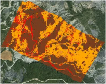
Fig. 12. Classification results: LAND(dark brown), ROAD(red),

ROCK(orange).

VEGETATION, but true positive values of ROAD decrease from 84.2% to 77.1% and the confusion withROCKincreases from 7.5% to 13.4%. In fact, the radiometry of roads are sen-sitive to tree shadows. The combination of the very high res-olution of RGBRAWand the time of the survey (early in the

morning) feeds the training set with bright and dark (shadow) radiometric values. On the contrary, lidar amplitude and width do not depend on the sun position. Superimposed on the orthoimage of Fig. 11, a 3-D landcover classification ob-tained with {RGBIGN, Amp, FWHM, dDTM} is presented in

Fig. 12 and 13.

6.3 Discussion

Finally, the quality of the classification depends mainly on the DTM accuracy (represented here as dDTM). Moreover,

within the framework of the methodology, it appears that a classification based on {Amp, FWHM, dDTM} is suitable,

but gives a worse accuracy than a classification based on

{dDTM, RGBRAW} or {dDTM, RGBIGN}. Used on their own,

full-waveform lidar data are relevant to discriminate vegeta-tion from non vegetavegeta-tion points, but the confusion between other classes remains not negligible. The amplitude and the width do not improve the classification accuracy if the ra-diometric features have a good separation between classes. Otherwise, the benefit is rather small, but in case of arte-facts in a class (like shadow) for which lidar measurements are not sensitive. Inversely, the use of poor radiometric fea-tures may alter the classification result of specific landscapes (hereROAD) where amplitude and width are well bounded. Even if amplitudes and widths appear poorly discriminant for the first level of 3-D landcover classification we used in addition to usual RGB images, we are quite convinced

Fig. 13. Classification results: LAND(dark brown), ROAD(red),

ROCK(orange) andVEGETATION(dark green).

that it could be more useful for lower hierarchical levels of 3-D landcover classification. For instance, these waveform parameters would probably give information on vegetation density, 3-D structure and type as well as local bared soil structure related to erodibility. These investigations will be the next steps of our research.

7 Conclusions

Firstly, the accuracy of the full-waveform lidar data on bad-lands is decimetric. Even if erosion dynamics on these land-scapes would require a centimetric accuracy to be studied yearly, DTMs generated from lidar survey are consistent for hydrological sciences at the catchment level. Moreover, we showed that these data permit to identify most of gullies and ridges of badland landscapes through geomorphological in-dices.

We focused this paper on generating and qualifying DTMs, but also on the automatic computation of a 3-D land-cover classification. We showed that lidar amplitude and width contain enough discriminative information on bad-lands to be classified inLAND,ROAD,ROCKandVEGETA

-TION with about 80% accuracy. Compared to usual cover classification from aerial or satellite images, 3-D land-cover classification is a new and interesting approach for hy-drologists since it allows to parametrise in a much direct way hydrological or erosion production parameters as, for instance, the plant cover C factor (Wischmeier et al., 1978). However, the introduction of image-based radiometric fea-tures combined to lidar ones in the classifier improved the accuracy of the classification (about 92%). They bring rele-vant discrimination between classes but cancelled most part of the value added from full-waveform data. This is mainly

due to the generality of the landcover classes we chose, but it would probably be more discriminant for more detailed land-cover classes.

Acknowledgements. The authors would like to deeply thank the

GIS Draix for providing the full-waveform lidar data and for helping in ground truth surveys. They are grateful to INSU for its support to GIS Draix through the ORE program.

Edited by: W. Wagner

References

Urban hydrology for small watersheds, Technical Release 55, United States Department of Agriculture, Natural Resources Conservation Service, Conservation Engineering Division, 2nd edn., 1986.

Antoine, P., Giraud, D., Meunier, M., and Ash, T. V.: Geological and geotechnical properties of the “Terres Noires” in southeast-ern France: weathering, erosion, solid transport and instability, Eng. Geol., 40, 223–234, 1995.

Antonarakis, A. S., Richards, K. S., Brasington, J., Bithell, M., and Muller, E.: Retrieval of vegetative fluid resistance terms for rigid stems using airborne lidar, J. Geophys. Res., 113, G02S07, doi:10.1029/2007JG000543, 2008.

Bailly, J., Lagacherie, P., Millier, C., Puech, C., and Kosuth, P.: Agrarian landscapes linear features detection from LiDAR eleva-tion profiles: applicaeleva-tion to artificial drainage network deteceleva-tion, Int. J. Remote Sens., 29(11–12), 3489–3508, 2008.

Baltsavias, E. P.: Airborne Laser Scanning: Basic relations and formulas, ISPRS J. Photogr. Remote Sens., 54(2–3), 199–214, 1999.

Bretar, F. and Chehata, N.: Terrain Modelling from lidar range data in natural landscapes: a predictive and Bayesian frame-work, Tech. rep., Institut G´eographique National, available at: http://hal.archives-ouvertes.fr/hal-00325275/fr/, 2008.

Bryan, R. and Yair, A.: Perspectives on studies of badland geo-morphology, in: Badland Geomorphology and Piping, edited by Bryan R, Y. A., GeoBooks (Geo Abstracts Ltd), Norwich, UK, 1–12, 1982.

Chang, C.-C. and Lin, C.-J.: LIBSVM: a library for support vec-tor machines, software available at: http://www.csie.ntu.edu.tw/

∼cjlin/libsvm, 2001.

Charleux-Demargne, J.: Valorisation des Mod`eles Num´eriques de Terrain en hydrologie. Qualit´e d’extraction d’objets et de car-act´eristiques hydrologiques `a partir des MNT. Utilisation pour l’estimation du r´egime de crues des bassins versants, Ph.D. the-sis, Universit´e de Marne-La-Vall´ee, France, 2001.

Chauve, A., Mallet, C., Bretar, F., Durrieu, S., Pierrot-Deseilligny, M., and Puech, W.: Processing full-waveform lidar data: model-ing raw signals, in: IAPRS, vol. 36 (Part 3/W52), Espoo, Finland, 2007.

Chauve, A., Bretar, F., Pierrot-Deseilligny, M., and Puech, W.: FULLANALYZE: A Research Tool for Handling, Processing and Analyzing Full-waveform Lidar Data, in: Proc. of the IEEE International Geoscience and Remote Sensing Symposium (IGARSS), Cape Town, South Africa, 2009.

Chowdhury, P. R., Deshmukh, B., and Goswami, A.: Machine Ex-traction of Landforms from Multispectral Images Using Texture

and Neural Methods, in: Proc. of the International Conference on Computing: Theory and Applications, Washington DC, USA, 721–725, 2007.

Cobby, D. M., Mason, D. C., and Davenport, I. J.: Image process-ing of airborne scannprocess-ing laser altimetry data for improved river flood modelling, ISPRS J. Photogr. Remote Sens., 56(2), 121– 138, 2001.

Cravero, J. and Guichon, P.: Exploitation des retenues et transport des s´ediments, La Houille Blanche, 3–4, 292–296, 1989. Descroix, L. and Mathys, N.: Processes, spatio-temporal factors

and measurements of current erosion in the French Southern Alps: a review, Earth Surface Processes and Landforms, 28 (9), 993–1011, 2003.

Edwards, D.: Some effects of siltation upon aquatic macrophyte vegetation in rivers, Hydrobiologia, 34 (1), 29–38, 1969. H¨ofle, B. and Pfeifer, N.: Correction of laser scanning intensity

data: Data and model-driven approaches, ISPRS J. Photogr. Re-mote Sens., 62(6), 415–433, 2007.

Hollaus, M., Wagner, W., and Kraus, K.: Airborne laser scanning and usefulness for hydrological models, Adv. Geosci., 5, 57–63, 2005,

http://www.adv-geosci.net/5/57/2005/.

Hsu, C.-W. and Lin, C.-J.: LIBSVM: a library for Support Vec-tor Machine, software available at: http://www.csie.ntu.edu.tw/

∼cjlin/libsvm, 2001.

Huang, C., Davis, L., and Townshend, J.: An assessment of sup-port vector machines for land cover classification, Int. J. Remote Sens., 22(4), 725–749, 2002.

Jacome, A., Puech, C., Raclot, D., Bailly, J., and Roux, B.: Ex-traction d’un mod`ele num´erique de terrain par photographies par drone, Revue des Nouvelles Technologies de l’Information, 79– 99, 2008.

James, L., Watson, D., and Hansen, W.: Using LiDAR data to map gullies and headwater streams under forest canopy: South Car-olina, USA, CATENA, 71(1), 2007.

Journel, A. and Huijbregts, C.: Mining Geostatistics, Academic Press, London, 610 pp., 1978.

Jutzi, B. and Stilla, U.: Range determination with waveform record-ing laser systems usrecord-ing a Wiener Filter, ISPRS J. Photogr. Re-mote Sens., 61, 95–107, 2006.

Kaasalainen, S., Hyyppa, H., Kukko, A., Litkey, P., Ahokas, E., Hyyppa, J., Lehner, H., Jaakkola, A., Suomalainen, J., Akuj¨arvi, A., Kaasalainen, M., and Pyysalo, U.: Radiometric Calibra-tion of LIDAR Intensity With Commercially Available Reference Targets, IEEE T. Geosci. Remote Sens., 47, 588–598, 2009. Kasser, M. and Egels, Y.: Digital Photogrammetry, Taylor &

Fran-cis, 2002.

King, C., Baghdadi, N., Lecomte, V., and Cerdan, O.: The applica-tion of Remote Sensing data to monitoring and modelling of soil erosion, CATENA, 62(2–3), 79–93, 2005.

Kirchhof, M., Jutzi, B., and Stilla, U.: Iterative processing of laser scanning data by full waveform analysis, ISPRS J. Photogr. Re-mote Sens., 63(1), 99–114, 2008.

K¨othe, R. and Lehmeier, F.: SARA System – System zur Automa-tischen Relief-Analyse, 11–21, 1994.

Lantuejoul, C.: Geostatistical Simulation: Models and Algorithms, Springer Verlag, Berlin, Germany, 256 pp., 2002.

Lillesand, T. and Kiefer, R.: Remote Sensing and Image interpreta-tion, John Wiley & Sons, 721 pp., 1994.

Malet, J., Auzet, A., Maquaire, O., Ambroise, A., Descroix, L., Esteves, M., Vandervaere, J., and Truchet, E.: Investigating the influence of soil surface characteristics on infiltration on marly hillslopes, Earth Surf. Proc. Landf., 28(5), 547–560, 2003. Mallet, C. and Bretar, F.: Full-Waveform Topographic Lidar:

State-of-the-Art, ISPRS J. Photogr. Remote Sens., 64, 1–16, 2009. Mallet, C., Bretar, F., and Soergel, U.: Analysis of full-waveform

li-dar data for classification of urban areas, Photogrammetrie Fern-erkundung GeoInformation (PFG), 5, 337–349, 2008.

Mason, D. C., Cobby, D. M., Horritt, M. S., and Bates, P. D.: Flood-plain friction parameterization in two-dimensional river flood models using vegetation heights derived from airborne scanning laser altimetry, Hydrol. Proc., 17(9), 1711–1732, 2003. Mathys, N.: information available: http://www.grenoble.cemagref.

fr/etna/oreDraix/oreDraix.htm, 2004.

Mathys, N., Brochot, S., and Meunier, M.: L’´erosion des Terres Noires dans les Alpes du Sud : contribution l’estimation des valeurs annuelles moyennes (bassins versants exp´erimentaux de Draix, Alpes-de-Haute-Provence, France), Revue de g´eographie alpine, 17–27, 1996.

Mathys, N., Brochot, S., Meunier, M., and Richard, D.: Erosion quantification in the small marly experimental catchments of Draix (Alpes de Haute Provence, France). Calibration of the ETC rainfall-runoff-erosion model, CATENA, 50(2–4), 527– 548, 2003.

McKean, J. and Roering, J.: Objective landslide detection and sur-face morphology mapping using high-resolution airborne laser altimetry, Geomorphology, 57(3–4), 331–351, 2004.

Murphy, P., Meng, J. O. F., and Arp, P.: Stream network mod-elling using lidar and photogrammetric digital elevation models: a comparison and field verification, Hydrol. Proc., 22 (12), 1747– 1754, 2008.

Nadal-Romero, E., Regu´es, D., Marti-Bono, C., and Serrano-Muela, P.: Badland dynamics in the Central Pyrenees: temporal and spatial patterns of weathering processes, Earth Surf. Proc. Landf., 32(6), 888–904, 2007.

O Callaghan, J. F. and Mark, D. M.: The extraction of drainage networks from digital elevation data, Comput. Vision Graphics Image Process., 28, 323–244, 1984.

O’Loughlin, E.: Prediction of surface saturation zones in natural catchments by topographic analysis, Water Resour. Res., 22(5), 794–804, 1986.

Oostwoud, W. D. and Ergenzinger, P.: Erosion and sediment trans-port on steep marly hillslopes, Draix, Haute-Provence, France: an experimental field study, CATENA, 33(22), 179–200, 1998. Paparoditis, N., Souchon, J.-P., Martinoty, G., and

Pierrot-Deseilligny, M.: High-end aerial digital cameras and their im-pact on the automation and quality of the production workflow, ISPRS J. Photogr. Remote Sens., 60, 400–412, 2006.

Pilgrim, D. H. (ed.): Australian rainfall and runoff, Institution of Engineers, Canberra, Australia, 1987.

Pontil, M. and Verri, A.: Properties of support vector machines, Tech. Rep. AIM-1612, MIT, Cambridge, USA, 1997.

Puech, C.: Utilisation de la t´el´ed´etection et des mod`eles num´eriques de terrain pour la connaissance du fonctionnement des hy-drosyst`emes, Habilitation `a diriger des recherches, Grenoble University, 2000.

Quinn, P., Beven, K., Chevallier, P., and Planchon, O.: The predic-tion of hillslope flow paths for distributed hydrological modelling using digital terrain models, Hydrol. Proc., 5(1), 59–79, 1991. Regues, D. and Gallart, F.: Seasonal patterns of runoff and

ero-sion responses to simulated rainfall in a badland area in Mediter-ranean mountain conditions (Vallcebre, Southeastern Pyrenees), Earth Surf. Proc. Landf., 29(6), 755–767, 2004.

Reitberger, J., Krzystek, P., and Stilla, U.: Analysis of full wave-form LIDAR data for the classification of deciduous and conifer-ous trees, Int. J. Remote Sens., 29, 1407–1431, 2008.

Schultz, G. and Engman, E., eds.: Remote Sensing in Hydrology and Water Management, Springer-Verlag, Berlin, Germany, 484 pp., 2000.

Sithole, G. and Vosselman, G.: Experimental Comparison of Fil-ter Algorithms for Bare-Earth Extraction from Airborne Laser Scanning Point Clouds, ISPRS J. Photogr. Remote Sens., 59(1– 2), 85–101, 2004.

Torri, D. and Rodolfi, G.: Badlands in changing environments: an introduction, CATENA, 40(2), 119–125, 2000.

Wagner, W., Ullrich, A., Ducic, V., Melzer, T., and Studnicka, N.: Gaussian Decomposition and calibration of a novel small-footprint full-waveform digitising airborne laser scanner, ISPRS J. Photogr. Remote Sens., 60(2), 100–112, 2006.

Wagner, W., Hollaus, M., Briese, C., and Ducic, V.: 3D vegeta-tion mapping using small-footprint full-waveformairborne laser scanners, Int. J. Remote Sens., 29(5), 1433–1452, 2008a. Wagner, W., Hyyppa, J., Ullrich, A., Lehner, H., Briese, C., and

Kaasalainen, S.: Radiometric calibration of full-waveform small-footprint airborne laser scanners, in: IAPRS, vol. 37(Part 1), Bei-jing, China, 2008b.

Walling, D.: Soil erosion research methods., chap. Measuring sed-iment yield from river basins,, Soil and water conservation soci-ety, Iowa, USA, 39–73, 1988.

Wischmeier, W. and Smith, D.: Predicting rainfall erosion losses: a guide to conservation planning - Agriculture Handbook, 537, US Dept Agric., Washington DC, USA, 1978.

Zevenbergen, L. and Thorne, C.: Quantitative Analysis of Land Sur-face Topography, Earth Surf. Proc. Landf., 12, 47–56, 1987. Zhang, L., O’Neill, A. L., and Lacey, S.: Modelling approaches

to the prediction of soil erosion in catchments, Environ. Softw., 11(1–3), 123–133, 1996.

Zwally, H. J., Schutz, B., Abdalati, W., Abshire, J., Bentley, C., Brenner, A., Bufton, J., Dezio, J., Hancock, D., Harding, D., Herring, T., Minster, B., Quinn, K., Palm, S., Spinhirne, J., and Thomas, R.: ICESat’s laser measurements of polar ice, atmo-sphere, ocean, and land, J. Geodynam., 34(3–4), 405–445, 2002.