HAL Id: hal-03066937
https://hal.archives-ouvertes.fr/hal-03066937
Submitted on 15 Dec 2020
HAL is a multi-disciplinary open access
archive for the deposit and dissemination of
sci-entific research documents, whether they are
pub-lished or not. The documents may come from
teaching and research institutions in France or
abroad, or from public or private research centers.
L’archive ouverte pluridisciplinaire HAL, est
destinée au dépôt et à la diffusion de documents
scientifiques de niveau recherche, publiés ou non,
émanant des établissements d’enseignement et de
recherche français ou étrangers, des laboratoires
publics ou privés.
Assessment of CNN-based Methods for Poverty
Estimation from Satellite Images
Robin Jarry, Marc Chaumont, Laure Berti-Équille, Gérard Subsol
To cite this version:
Robin Jarry, Marc Chaumont, Laure Berti-Équille, Gérard Subsol. Assessment of CNN-based
Meth-ods for Poverty Estimation from Satellite Images. 11th IAPR International Workshop on Pattern
Recognition in Remote Sensing (PRRS) in conjunction with the International Conference on Pattern
Recognition (ICPR 2020)„ Jan 2021, Milan, Italy. �hal-03066937�
Assessment of CNN-based Methods for Poverty
Estimation from Satellite Images
Robin Jarry1,2[0000−0003−4118−3619], Marc Chaumont2,3[0000−0002−4095−4410], Laure Berti-Équille4[0000−0002−8046−0570], and Gérard Subsol2[0000−0002−7461−4932]
1 French Foundation for Biodiversity Research (FRB), Montpellier, France 2 Research-Team ICAR, LIRMM, Univ. Montpellier, CNRS, Montpellier, France
3 University of Nîmes, France
4 ESPACE-DEV, Univ. Montpellier, IRD, UA, UG, UR, Montpellier, France
Abstract. One of the major issues in predicting poverty with satellite images is the lack of fine-grained and reliable poverty indicators. To address this prob-lem, various methodologies were proposed recently. Most recent approaches use a proxy (e.g., nighttime light), as an additional information, to mitigate the prob-lem of sparse data. They consist in building and training a CNN with a large set of images, which is then used as a feature extractor. Ultimately, pairs of extracted feature vectors and poverty labels are used to learn a regression model to predict the poverty indicators.
First, we propose a rigorous comparative study of such approaches based on a unified framework and a common set of images. We observed that the geographic displacement on the spatial coordinates of poverty observations degrades the pre-diction performances of all the methods. Therefore, we present a new method-ology combining grid-cell selection and ensembling that improves the poverty prediction to handle coordinate displacement.
1
Introduction
Estimating poverty indicators is essential for the economy and political stability of a nation. These indicators are usually evaluated by surveying the population and ask-ing people many questions. This requires a heavy organization, takes a long time, is sometimes only limited to easily accessible areas, and may be subjective. Therefore, solutions were proposed to estimate poverty at a large scale in an easier and faster way by using observational data, i.e., with no direct interaction with the people.
Satellite images give a quite precise observational overview of the planet. As early as 1980, Welch [Welch, 1980] monitored urban population and energy utilization pat-terns from the images of the first Landsat satellites. Since 1999 and 2013 respectively, Landsat 7 and 8 satellite series cover the entire Earth surface with a temporal resolution of 16 days and a spatial resolution of 15 to 30 meters depending on the spectral bands (8 for Landsat 7 and 11 for Landsat 8). Since 2014, Sentinel satellite series generate images with a spatial resolution of 10 meters. It is then possible to get remote-sensing data with a high time-frequency and a good spatial resolution.
Nevertheless, estimating the local wealth or poverty indicator rather than general value over a country is a very challenging problem. This requires the mapping of the
observational data (i.e., the pixel intensity of a satellite image) and the poverty indicator precisely located. In some cases, numerous indicators can be available. For example, in [Babenko et al., 2017], 350,000 poverty indicators are collected in two surveys over the city of Mexico or, in [Engstrom et al., 2017], 1,300 ground-truth poverty indicators are obtained for a limited 3,500 km2area of Sri Lanka. With a large number of indica-tors, direct supervised training with high-resolution daytime satellite images becomes possible, in particular with Deep-Learning techniques. Unfortunately, the number of such indicators is usually low in most countries, especially in developing ones. For ex-ample, only 770 poverty indicators are reported in 2016 for Malawi5with an area of more than 118, 000 km2. In 2013, Chandy [Chandy, 2013] reported in general terms that almost two-fifths of the countries do not perform at least one income survey every 5 years. Based on this observation, a direct Machine-Learning approach, processing a set of geolocalized satellite images associated with the corresponding poverty indica-tors would inevitably lead to over-fitting, and then very bad generalization (e.g., see [Ngestrini, 2019]).
But, in 2016, Jean et al. [Jean et al., 2016] proposed an accurate and scalable method based on Deep-Learning to estimate local poverty from satellite imagery, based on sparse socio-economic data. They managed to solve the problem of the limited number of poverty indicators by using a Transfer Learning technique. It consists in training a Convolutional Neural Network (CNN) on one task and then applying the trained CNN to a different but related task. Since this seminal work, many papers have been pub-lished with either applying or extending the original algorithm, or propose some vari-ants of Deep-Learning techniques. In particular, Ermon Group6at Stanford University proposed different methods to tackle the problem (see [Yeh et al., 2020] for their latest results).
The difficulty is then to compare all the available methods as they do not use the same input data and they are not evaluated with the same set of parameters. In this paper, we propose to assess the methods with a common framework in order to analyze their performances, understand the limitations of the available data (both images and indicators), and evaluate whether combining them would improve the results. In Section 2, we describe three methods we selected in this line of research. In Section 3, we present the common framework to assess fairly the performances of the methods. In Section 4, we discuss adapting the methods to improve the performances. Conclusion and future work are presented in Section 5.
2
Description of the Selected CNN-based Methods
Transfer Learning emerged recently as an efficient way to deal with a limited number of poverty indicators. For our application, proxy data related to poverty and available in large quantities can be used to train a CNN for classifying satellite images accordingly. By taking a specific layer of the resulting CNN, we can extract a feature vector that characterizes the input satellite image with respect to its correlation with the
corre-5Living Standard Measurements Study, Malawi 2016: https://microdata.worldbank.
org/index.php/catalog/2939.
sponding proxy data. As proxy data are chosen to be related to poverty, we can assume that the feature vector is an appropriate representation of poverty in the image.
Finally, we can compute the feature vectors of satellite images at the sparse locations of the limited set of poverty indicators, and perform a regression between the vectors and the poverty indicators. This process can be done efficiently despite a limited number of locations and it can establish a relationship between the satellite images and the poverty indicators.
A major issue is then to select relevant proxy data. Several solutions have been proposed and we review three of them in the following sections.
2.1 Nighttime Light
The concept of using Transfer Learning to estimate poverty from satellite images was proposed in [Jean et al. 2016]. In this work, the authors used nighttime light values (NLV), which are known, since many years, to be a good proxy for poverty evaluation (see for example, [Elvidge et al., 1997], [Doll et al., 2000] or [Chen and Nordhaus, 2011]).
NLV data set is provided by the Earth Observation Group7and the corresponding images are extracted from Google Static Map8, at 2.5 meters of resolution.
The authors introduce a CNN architecture to classify daytime satellite images by NLV. Three classes are used for low, medium, and high NLV [Jean et al., 2016, Supple-mentary Materials]. The CNN is based on a VGG-F architecture [Wozniak et al., 2018] and is pre-trained on the ImageNet dataset. Next, the network is fine-tuned on the train-ing data set, which consists of 400,000 [Xie et al., 2016] images, each of them covertrain-ing a 1km2area in Africa.
[Perez et al., 2017] is an extension of the previous research based on Landsat im-ages. It shows that despite the lower resolution of Landsat images, the model accuracy is higher than the one of the previous benchmarks.
2.2 Land Use
In [Ayush et al., 2020], the authors assume that land use, and specifically the manufac-tured objects observed in a satellite image emphasize the wealthiness of an area. The authors trained a CNN on a land use detection and classification task, to extract a fea-ture vector related to poverty. As proxy data, they used the xView data set9consisting of very high-resolution images (0.3 m) annotated with bounding boxes defined over 10 main classes (building, fixed-wing aircraft, passenger vehicle, truck, railway vehi-cle, maritime vessel, engineering vehivehi-cle, helipad, vehicle lot, construction site) and 60 sub-classes. As the size of the objects in a satellite image may vary (e.g., a truck is much smaller than a building), the network used YoloV3, with DarkNet53 backbone architec-ture [Redmon and Farhadi, 2018], which allows the detection at 3 different scales. This network is pre-trained on ImageNet and fine-tuned on the xView data set. Since it was
7NOAA Earth Observation Group Website:https://ngdc.noaa.gov/eog/
8Google Static Map, getting started Web page:https://developers.google.com/maps/
documentation/maps-static/start.
trained on a detection/classification task, a single satellite image may have several de-tection results, depending on the number of objects in the image. Thus, the input image may be associated with multiple feature vectors, one for each detection. The authors further explore this additional information by different combinations of the feature vec-tors.
2.3 Contrastive Spatial Analysis
In [Jean et al., 2019], the idea is to be able to cluster homogeneous-looking areas and assume that some clusters will be specific to poor areas. Contrary to the two previous approaches, this method is based on an unsupervised task. A CNN model is trained with the aim of learning a semantic representation of an input image according to the following constraints: (i) If two sub-parts of an image are close spatially, they must have a similar semantic representation (i.e., feature vectors); and (ii) If two sub-parts of an image are far apart, they must have a dissimilar semantic representation.
The data set is a set of image triplets (a, n, d), where a, n, and d are tiles that are sampled randomly from the same image.
More precisely, the neighbor tile n is sampled randomly in a given neighborhood of a, the anchor tile and d, the distant tile is sampled randomly outside of a’s neighbor-hood. The objective is to minimize the following cost function using the CNN:
L(ta,tn,td) = max (0, kta− tnk2− kta− tdk2+ m) (1) where ta, tn and td are the feature vectors produced by the CNN for the anchor tile a, the neighbor tile n, and the distant tile d respectively. m is the margin to enforce a minimum distance. During the minimization process, if tnis too far from tacompared to td(using the Euclidean distance), then tnwill be generated to get closer to ta, and td will get more distant from ta. The equilibrium is obtained when tdis in the hypersphere with radius kta− tnk + m. The CNN is a modified version of ResNet-18 taking the three tiles as inputs.
2.4 Regression Step
All the previous methods aim to produce a feature vector representation of a satellite image that should represent poverty to a certain extend. The first approach uses a feature vector that estimates NLV from the satellite images. The second approach uses a fea-ture vector that estimates land use. The third approach uses a feafea-ture vector that empha-sizes the differences between two satellite images. Throughout the paper, we will name the three methods, Nighttime Light,Land Use, andContrastive respectively. For each method, a Ridge regression model is trained with the pairs of feature vectors (obtained from the corresponding method) and the poverty indicators. The feature vectors are gen-erated from the images of the sparse locations where some poverty indicators are avail-able. We select the Ridge regression model, that is as close as possible to the method-ology exposed in [Jean et al., 2016], [Jean et al., 2019], and [Ayush et al., 2020].
2.5 Comparison Issues
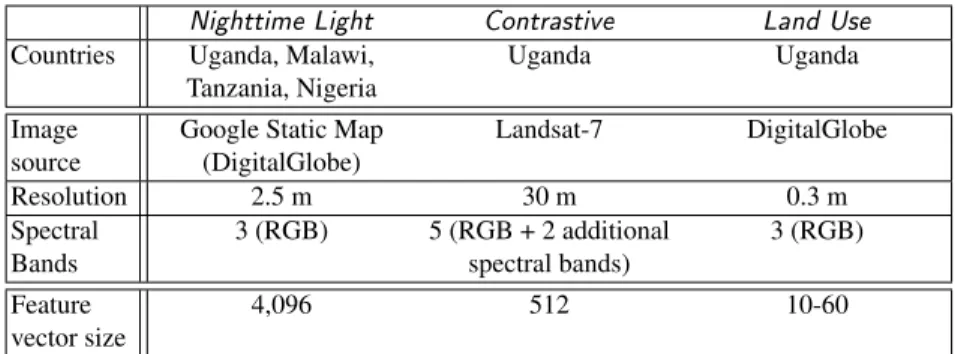
The three methods aforementioned may seem to offer comparable results from the re-sults reported, but as a matter of fact, they differ greatly by the choice of the satellite images, proxy data, and feature vector parameters as we can see in Table 1.
Nighttime Light Contrastive Land Use Countries Uganda, Malawi,
Tanzania, Nigeria
Uganda Uganda
Image source
Google Static Map (DigitalGlobe) Landsat-7 DigitalGlobe Resolution 2.5 m 30 m 0.3 m Spectral Bands 3 (RGB) 5 (RGB + 2 additional spectral bands) 3 (RGB) Feature vector size 4,096 512 10-60
Table 1. Differences between the input data and parameters used in the three methods.
Notice that the images do not share the same resolution and the structures and ob-jects captured in the images do not have the same scale. Moreover, in [Jean et al., 2019], the images contain 5 spectral bands, whereas the other methods process standard RGB images.
Experiments reported in [Perez et al., 2017] have shown that lower resolution im-ages and additional spectral bands could influence poverty estimation. With this con-sideration in mind, we can assume that the image resolution and the number of spectral bands are significant features that must be commonly set before any method compari-son.
Additionally, the size of the feature vectors generated by the CNN differs for each method. As it is difficult to know the influence of this parameter on the final R2score, we set the size to be identical across the different methods, to provide a fair comparison.
3
A Common Framework to Assess the CNN-based Methods
Our goal is to compare the three methods consistently and fairly with a common frame-work, to expose their benefits and limitations. Therefore, we decided to use the same satellite image source, the same image dimension and scale, the same regression steps, and the same socio-economic indicators. Doing so, we can compare which approach better emphasizes the poverty and if an unsupervised method, i.e., without proxy data, can outperformNighttime LightorLand Usemethods.
Before discussing the framework, it is important to notice that the poverty indicators given in the available surveys are artificially moved from their actual position, which may lead to biasing the results.
Fig. 1. Geographic displacement procedure performed on LSMS socio-economic surveys.
Surveying operators add a random geographic displacement up to 10km on latitude and longitude from the location where the socio-economic indicator is evaluated, to pro-tect the anonymity of respondents (see [Burgert et al., 2013]10). In the example given in Figure 1, the poverty indicators of a village are distributed over a 10km × 10km sur-rounding area. This means that the actual poverty indicator can be significantly different from the reported one in the survey.
3.1 Framework Specifications
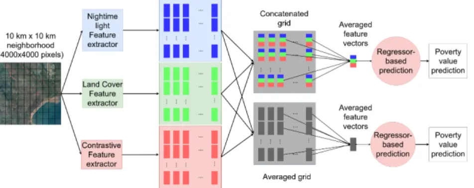
We can represent the three methods as the global pipeline shown in Figure 2. In the com-mon framework we propose, the algorithm operates over a 10 km×10 km area around a given input location (i.e. latitude and longitude coordinates) with a corresponding poverty indicator. It takes as input a 4,000×4,000 pixels satellite image centered on the considered location. This ensures that the true indicator location is indeed in the image. Each image is then split into 100 sub-images (of 400 × 400 pixels), each one covering a 1 km×1 km area according to a regular grid. The sub-images are then processed by
10This document shows how Demographic and Health Surveys are modified, and claims that the
Living Standards Measurement Study, our survey provider, performs the same anonymization policy.
a Deep Learning feature extractor specific to a selected method (Nighttime Light,Land
Use,Contrastive) in order to produce a fixed-size feature vector. Finally, the feature vectors are averaged and sent to a Ridge regressor, which returns the poverty estimation value for the 1km × 1km area centered in the input location.
3.2 Data Description
Satellite images are used for both feature extractor training and poverty indicator esti-mation using regression. Some proxy data are also needed to buildNighttime Lightand
Land Usefeature vectors.
Satellite images: Since we want to compare the approaches, the images used to build all the feature extractor and output the socio-economic estimates are provided by the Google Static Map API11. The satellite images used are 400 × 400 pixels, covering a 1km2 area (2.5 meters resolution) with the classical RGB color channels. For each location in the survey, we use the same type of images to build a larger one that covers a 10km × 10km neighboring area.
Proxy data forNighttime Lightmethod: As in [Jean et al., 2016], we used the 1km resolution world map of NLV, provided by the Earth Observation Group in 201312. No-tice that afterward, the Earth Observation Group has provided 500m resolution world maps. Unfortunately, there is no reliable time reference mentioned and associated with Google Static Map images so we assume that 2013 NLV data are roughly consistent with Google Static Map images. Finally, 71,000 daytime images were randomly se-lected from the NLV world map in Africa.
Proxy data forLand Usefeature extractor:
The xView dataset image resolution (0.3 m) is much higher than GSM one (2.5 m), which prevents us from using the object detection methodology based on xView dataset. We then adapted the idea and use a global land use classifier which outputs a single value instead of a set of feature vectors corresponding to each detected object.
We used land use labels provided in the Eurosat data set [Helber et al., 2018]. It consists of almost 30,000 satellite images of European places, labeled into 10 classes: sea lake, river, residential, permanent crop, pasture, industrial, highway, herbaceous vegetation, forest, and annual crop. The authors provided a GeoTIFF data set13, includ-ing the locations of all images, we simply used these locations and downloaded the corresponding Google Static Map API images.
Proxy data forContrastivefeature extractor: Since it is an unsupervised method, no proxy data is required. Therefore, we used the poverty indicator location to generate 4,000 × 4,000, images with 2.5 meters resolution. Then, for each image, we randomly sample 100 anchor, neighbor, and distant image triplets, with the same size, area cov-erage, and channel as introduced earlier. We set the neighborhood size to 400 pixels, so
11Google Static Map getting started web page: https://developers.google.com/maps/
documentation/maps-static/start.
12Nighttime Light world map: https://www.ngdc.noaa.gov/eog/dmsp/
downloadV4composites.html.
13GeoTIFF data set provided by [Helber et al., 2018]: https://github.com/phelber/
the central pixel of each neighbor image (resp. distant image) is less (resp. more) than 400 pixels away from the anchor image. The overall process generates 77,000 triplets.
Poverty indicators: We used the poverty indicators from LSMS surveys14. We fo-cus on the 2016 Malawi survey and consider the natural logarithm of the consumption expenditures as the poverty indicator. Note that the surveys are designed in two steps. The country is divided into clusters, and then, several households are surveyed within each cluster. In the resulting survey, only the clusters coordinates are reported (and ran-domly displaced for anonymization purposes, as explained earlier). In our experiments, we use the 770 clusters provided by the survey to train and test the poverty prediction models at the cluster level.
3.3 Metrics and Evaluation Goal
Performances of CNNs: We use the accuracy metric for assessing the classification task which allows us to compute feature vectors inNighttime Light andLand Use. It is defined as follows: A= 1 N N
∑
i=1 δ (yi, ˆyi) (2) with y = (yi)i∈{1,...,N} (resp. ˆy= ( ˆyi)i∈{1,...,N}) the true (resp. predicted) NLV value or land use, N the number of predictions, and δ the Kronecker delta. SinceContrastivedoes not make any prediction, we can not use accuracy to measure its quality performance.Performances of the Ridge regressor: We consider y = (yi)i∈{1,...,N} (resp. ˆy= ( ˆyi)i∈{1,...,N}) as the true (resp. predicted) poverty indicator and N be the number of predictions. Similarly to previous work, we used the R2score, also called coefficient of determination, defined as follows:
R2= 1 −∑ N
i=1(yi− ˆyi)2 ∑Ni=1( ¯y− yi)2
. (3)
R2aims to measure the mean squared error (numerator) over the variance (denom-inator). As a universal and classical metric, it corresponds to the amount of variance explained by the model.
Cross-validation: The usual train/test splitting process leads to too small data sets impacting the quality of the learning and decreasing the performances. The sparsity of poverty indicators causes some differences between training and testing data distribu-tions. Therfore, the results obtained from a given train/test split can be very different from the ones obtained with other train/test splits. To avoid this problem, we use 10-fold cross-validation and average the scores.
3.4 Implementation
We ran our experiments using a workstation with 32 Gb, Intel Xeon 3.6GHz 12 cores, and a NVIDIA Quadro GV100 graphic card. We used the Python TensorFlow 2.x li-brary.
14Living Standard Measurements Study, Malawi 2016: https://microdata.worldbank.
The three CNNs are based on the VGG16 architecture, followed by a fully con-nected layer (used to extract the features) and ended with the classification layer. The VGG16 architecture is pre-trained on ImageNet. We used stochastic gradient descent as optimizer.
All the image pixel values are scaled from 0 to 1 and a horizontal and vertical flip is randomly applied during the training phase as data-augmentation. At the end of each epoch, a validation step is done. The feature extractors are generated with the weights that optimize the validation accuracy when available (Nighttime LightandLand Use) or the validation loss (Contrastive). The training phase ran for 100 epochs and lasts for 18 hours forNighttime Light, 13 hours forLand Use, and 3 hours forContrastive.
The feature vectors generated by the feature extractors have d = 512 dimensions. We use the Ridge regression with regularization parameters α chosen among the values {10−4, 10−3, . . . , 105}.
3.5 Results
Table 2 gives R2 scores which can be considered as baseline results. The first col-umn contains the results obtained when only the feature vector corresponding to the anonymized position is used for regression (without considering the 10km × 10km neighborhood). The second column contains the results obtained when all the feature vectors corresponding to an input image in the 10km × 10km neighborhood are av-eraged. Regardless of the feature extractor, we can observe across the methods that there is a significant difference between the R2score when all the positions are consid-ered compared to the score obtained with a single feature vector from the anonymized position. The gain ranges from +0.04 to +0.09. Note that the R2values for the three state-of-the-art approaches are similar, with 0.47, 0.46, and 0.45. Nevertheless, the R2 standard deviation remains high and prevents a fair ranking of the approaches.
anonymized Position All Positions α Nighttime Light 0.404 ±0.07 0.449±0.09 102 Land Use 0.383 ±0.08 0.47±0.08 103 Contrastive 0.385±0.07 0.462±0.08 102
Table 2. R2scores of the three poverty prediction methods, evaluated on the test data set (10-folds cross-validation).
4
How to Improve the Results?
Let us investigate two ways to ameliorate the methods’ prediction. The first proposition consists in handling the spatial perturbation of the coordinates. The second approach consists in combining the three approaches.
4.1 Handling the Geographic Perturbation
The random perturbation injected in the spatial coordinates of the surveyed poverty indicators may directly affect the prediction results. Therefore, we propose a 2-step method with two variants each, adapting the following step of the framework exposed in Section 3.1: For each position in the survey, (1) We consider all the 10km × 10km neighboring areas for feature extraction, and (2) We average the resulting feature vec-tors.
On the one hand, the first step allows capturing the true position of the poverty indicator. On the other hand, it captures also the 99 false positions of the poverty indi-cator, perturbing the most important information. The second step reduces drastically the amount of information. The resulting average feature vector is a summarized rep-resentation of the 10km × 10km neighborhood in which all the specific features are omitted.
Adaptation of Step (1) with grid-cell selection: Instead of considering all the 10km × 10km neighboring areas for each position in the survey, we select specific cells in the grid of the neighborhood. The selection is based on the inhabitant num-ber from WorldPop15 and NLV. More precisely, we keep the cells that correspond to: (a) The n most populated places, and (b) The n highest NLV, with n varying in {1, 5, 10, 20, 40, 60, 80}.
After this first adaptation, we exclude "no mans’ land" areas where there is no plau-sible position for a poverty indicator. Then, the feature extractors process only the se-lected cells and return n feature vectors per position in the survey.
Adaptation of Step (2) without averaging the feature vectors: For each position in the survey: (a) We average the n feature vectors and compare with the case where (b) The n feature vectors are used for regression. In the latter case, the n feature vectors are annotated with the poverty indicator collected at the corresponding position in the survey. Doing so, we ensure that the specific features captured in all the feature vectors are processed by the regression model.
4.2 Combining the Approaches
There is a large body of research on ensembling methods in the literature. As a starting point, we investigate two simple and straightforward ways of combining the approaches illustrated, in Figure 3. Future work will explore and test other ensembling methods.
Given the entire grid (10km × 10km area), a feature extractor outputs one vector for each cell. Please note that some cells may not be processed because of the grid-cell selection, depending on their respective inhabitant number (1a) or NLV (1b). Given a grid-cell, i.e., a sub-image of 400 × 400 pixels that covers a 1km2area, each of the three feature extractors returns a feature vector. Then, the three feature vectors are either averaged (Ensembling Averaged) or concatenated (Ensembling Concatenated).
4.3 Experiments and Analysis
Performances of feature extractors: The CNNs are used to extract features from im-ages. Therefore, their respective accuracy values are not used to determine whether or
not they are good classifiers. However, the accuracy metric can be used as an indi-rect measure to indicate the degree of consistency between the features generated by the CNNs, according to the classification problem (only forNighttime LightandLand Use approaches).Nighttime Light reaches 64% of accuracy on the validation data set, whereasLand Usereaches 97%. As mentioned earlier, instead of the accuracy measure, we use the R2score for evaluatingContrastive’s performance on the poverty prediction task.
Fig. 3. Ensembling pipeline. Similar to figure 2, with an intermediate step of either concatenation or averaging, represented by the gray grids. Note that that the previous adaptation (1) and (2) are not shown, for the sake of clarity.
R2of SOTA methods R2of our methods handling geographic perturbation Single anonymized position Averaging across all positions Population-based grid-cell selection n= 20 and averaging NLV-based grid-cell selection n= 20 and averaging Random grid-cell selection n= 20 and averaging Population-based grid-cell selection n= 20 and not averaging Nighttime Light 0.404± 0.07 0.449± 0.09 0.496± 0.09 0.487 ± 0.08 0.411± 0.07 0.379±0.08 Land Use 0.383±0.08 0.47± 0.08 0.483± 0.08 0.466± 0.08 0.403± 0.05 0.35±0.07 Contrastive 0.385±0.07 0.462± 0.08 0.486± 0.04 0.464± 0.06 0.388± 0.05 0.313±0.04 Ensembling Concatenated 0.44±0.08 0.48± 0.09 0.491± 0.07 0.502± 0.08 0.429± 0.07 0.387±0.07 Ensembling Averaged 0.41± 0.08 0.47± 0.09 0.494± 0.07 0.487± 0.07 0.422± 0.05 0.378±0.07 Table 3. R2 scores for different grid-cell selection (column) and feature extractors (row). Best R2= 0.502 is obtained with the ensembling method by concatenation, with NLV-based grid-cell selection (n = 20).
Discussion on grid-cell selection: We can notice that the two grid-cell selection approaches have similar results, essentially because there is an overlap between the cells selected by each method.
When selecting the grid-cells, either based on the population criterion, or the NLV criterion, the average R2score increases up to +0.05 compared to the score obtained when using all the feature vectors. The highest increase is obtained with the population criterion. Each approach benefits from the population-based grid-cell selection. Only
Nighttime Light benefits from NLV-based grid-cell selection. Compared to the results obtained by averaging all the feature vectors, all the approaches give an average R2 above 0.48. At this stage, we can say that our grid-cell selection method slightly im-proves the results. By selecting the most likely true positions of the indicators in the survey, we add the geographical context. However, when considering the same pro-portion of geographical context, random grid-cell selection is still less efficient than population-based grid-cell selection or NLV-based grid-cell selection, from +0.06 to +0.1. This suggests naturally that capturing the true position improves the prediction of the model.
Discussion on averaging or not the feature vectors: With the same grid-cell selection, averaging the selected feature vectors leads to the best results and should be recommended. In Table 3, the same grid selection is applied for both columns 3 and 6, but the selected feature vectors are averaged (column 3) and the selected feature vectors are all processed (column 6) by the regression model. We can notice that averaging increases the R2score up to +0.15. The correct cell (correct position) with the correct poverty value may be masked by the 20 other feature vectors. This probably explains the poor performance of this approach.
Discussion on the ensembling approaches: Combining the approaches by con-catenation or averaging always improves the average R2score by +0.01 approximately. The best results are obtained with NLV-based grid-cell selection, with an average R2 reaching 0.50. However, the improvement is negligible. For example, when using the population-based grid-cell selection, there is no improvement compared toNighttime Lightalone.
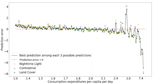
Next, we investigate whether an ensembling approach combining the three methods can significantly improve the results. For several test folds and all the ground truth data in each test fold, we compare the relative prediction error made by Nighttime Light,
Land Cover, andContrastive (shown in Figure 4, for one particular test fold). Then, for each ground truth observations, we select the prediction with the smallest prediction error. We average the R2score obtained with the best prediction over the test folds, and obtain R2= 0.6. This score is significantly higher than all the other results presented in Table 3. Thus, there is room for improvement by ensembling the methods.
Additionally, in Figure 4, we observe that, regardless of the feature extractor, the three approaches are slightly over-estimating the richness when the poverty is extreme, and give more erroneous predictions when the poverty is above 2.4$/day. This can be explained by a fewer number of poverty indicators that are greater than 2.4$/day in the learning set.
Fig. 4. Prediction error of the three feature extractors for one of the test fold with respect to the poverty level. The prediction is obtained by averaging all the feature vectors for a given position and applying the learnt regression model. Black line connects the best predictions among the three predictions for each test sample. Note that the X-axis is not linear.
5
Conclusion and Future Work
By providing a fair comparison between three state-of-the-art models for poverty pre-diction, we present several insightful results: (1) Such models produce similar results on the same framework. (2) The spatial perturbation injected in the coordinates of poverty indicators is a key issue that reduces significantly the prediction power of the models. By handling the spatial perturbation of the coordinates, our grid-cell selection method shows better performances and motivates future work to ameliorate the entire process. (3) Using anonymized coordinates from the surveys implies poverty prediction at a 10km × 10km scale (which can still capture the true position) rather than 1km × 1km scale. However, it prevents the use of very high-resolution images available to-day. Covering a 100 km2area with high-resolution images would necessitate very large images (4,000 × 4,000 with 2.5 meters resolution) that cannot be directly processed by a CNN. We believe that this opens several new research directions to handle noise and high-resolution images for CNN-based prediction models. (4) We showed that our combination of the three considered methods does not augment drastically the qual-ity performance. However, we experience that choosing the best prediction among the three methods leads to R2= 0.6. Thus, we claim that there exists a combination of the three methods that can give significant improvement of the R2score. As it is a choice on the prediction strategy, we believe that other or more sophisticated ensembling methods can be even more efficient. (5) Finally, the small size of the data set causes some differ-ences and discrepancies between the training and testing data sets, which are reflected by high standard deviation values during the cross-validation.
To pursue this work, we aim to propose a combination method that can reach higher R2 scores, eventually using multi-spectral imagery to estimate poverty indicators as other work in the literature. Using the fair benchmark for poverty prediction we pro-posed, we plan to explore the benefits of multi-spectral images compared to natural RGB images. Finally, other deep learning architectures may be more likely to give a better feature representation of images. Therefore, one of our goals will be to test and find an optimal architecture.
Acknowledgment
This research was partly funded by the PARSEC group, funded by the Belmont Forum as part of its Collaborative Research Action (CRA) on Science-Driven e-Infrastructures Innovation (SEI) and the synthesis centre CESAB of the French Foundation for Re-search on Biodiversity. This work was also partly funded by the French ANR project MPA-POVERTY.
References
[Ayush et al., 2020] Ayush, K., Uzkent, B., Burke, M., Lobell, D., and Ermon, S. (2020). Gen-erating interpretable poverty maps using object detection in satellite images. In Bessiere, C., editor, Proceedings of the Twenty-Ninth International Joint Conference on Artificial Intelli-gence, IJCAI-20, pages 4410–4416. International Joint Conferences on Artificial Intelligence Organization. Special track on AI for CompSust and Human well-being.
[Babenko et al., 2017] Babenko, B., Hersh, J., Newhouse, D., Ramakrishnan, A., and Swartz, T. (2017). Poverty mapping using convolutional neural networks trained on high and medium resolution satellite images, with an application in mexico. NIPS 2017 Workshop on Machine Learning for the Developing World.
[Burgert et al., 2013] Burgert, C. R., Colston, J., Roy, T., and Zachary, B. (2013). Geographic displacement procedure and georeferenced data release policy for the demographic and health surveys. DHS Spatial Analysis Reports No. 7. Calverton, Maryland, USA: ICF International. [Chandy, 2013] Chandy, L. (2013). Counting the poor: Methods, problems and solutions behind
the $1.25 a day global poverty estimates. Working Paper No. 337682, Developement Ini-tiatives & Brooking Institution. http://devinit.org/wp-content/uploads/2013/09/ Counting-the-poor11.pdf.
[Chen and Nordhaus, 2011] Chen, X. and Nordhaus, W. D. (2011). Using luminosity data as a proxy for economic statistics. Proceedings of the National Academy of Sciences, 108(21):8589– 8594.
[Doll et al., 2000] Doll, C. N. H., Muller, J.-P., and Elvidge, C. D. (2000). Night-time imagery as a tool for global mapping of socioeconomic parameters and greenhouse gas emissions. Ambio, 29(3):157–162.
[Elvidge et al., 1997] Elvidge, C., Baugh, K., Kihn, E., Kroehl, H. W., Davis, E., and Davis, C. (1997). Relation between satellite observed visible-near infrared emissions, population, economic activity and electric power consumption. International Journal of Remote Sensing, 18:1373–1379.
[Engstrom et al., 2017] Engstrom, R., Hersh, J., and Newhouse, D. (2017). Poverty from space: Using high-resolution satellite imagery for estimating economic well-being. Policy Re-search Working Paper; No. 8284, World Bank, Washington, DC. https://openknowledge. worldbank.org/handle/10986/29075 License: CC BY 3.0 IGO.
[Helber et al., 2018] Helber, P., Bischke, B., Dengel, A., and Borth, D. (2018). Introducing eu-rosat: A novel dataset and deep learning benchmark for land use and land cover classification. In IGARSS 2018-2018 IEEE International Geoscience and Remote Sensing Symposium, pages 204–207. IEEE.
[Jean et al., 2016] Jean, N., Burke, M., Xie, M., Davis, W. M., Lobell, D. B., and Ermon, S. (2016). Combining satellite imagery and machine learning to predict poverty. Science, 353(6301):790–794.
[Jean et al., 2019] Jean, N., Wang, S., Samar, A., Azzari, G., Lobell, D., and Ermon, S. (2019). Tile2vec: Unsupervised representation learning for spatially distributed data. In AAAI-19/IAAI-19/EAAI-20 Proceedings, pages 3967–3974. AAAI technical track : Machine Learning. [Ngestrini, 2019] Ngestrini, R. (2019). Predicting poverty of a region from satellite imagery
using cnns. Master’s thesis, Departement of Information and Computing Science, Utrecht Uni-versity. Unpublished,http://dspace.library.uu.nl/handle/1874/376648.
[Perez et al., 2017] Perez, A., Yeh, C., Azzari, G., Burke, M., Lobell, D., and Ermon, S. (2017). Poverty prediction with public landsat 7 satellite imagery and machine learning. NIPS 2017, Workshop on Machine Learning for the Developing World.
[Redmon and Farhadi, 2018] Redmon, J. and Farhadi, A. (2018). Yolov3: An incremental im-provement. CoRR, abs/1804.02767.
[Welch, 1980] Welch, R. (1980). Monitoring urban population and energy utilization patterns from satellite data. Remote Sensing of Environment, 9(1):1 – 9.
[Wozniak et al., 2018] Wozniak, P., Afrisal, H., Esparza, R., and Kwolek, B. (2018). Scene recognition for indoor localization of mobile robots using deep CNN. International Confer-ence on Computer Vision and Graphics.
[Xie et al., 2016] Xie, M., Jean, N., Burke, M., Lobell, D., and Ermon, S. (2016). Transfer learning from deep features for remote sensing and poverty mapping. 30th AAAI Conference on Artificial Intelligence.
[Yeh et al., 2020] Yeh, C., Perez, A., Driscoll, A., Azzari, G., Tang, Z., Lobell, D., Ermon, S., and Burke, M. (2020). Using publicly available satellite imagery and deep learning to understand economic well-being in Africa. Nature Communications, 11(1):2583.