Aeroacoustic measurement and analysis of transient supersonic hot nozzle flows

(1)

AEROACOUSTIC MEASUREMENT AND ANALYSIS OF TRANSIENT

SUPERSONIC HOT NOZZLE FLOWS

by

DANIEL ROBERT KIRK

Bachelor of Science in Mechanical Engineering

Rensselaer Polytechnic Institute, 1997

Submitted to the Department of Aeronautics and Astronautics in partial fulfillment of the requirements for the degree of

MASTER OF SCIENCE

in

AERONAUTICS AND ASTRONAUTICS

at the

MASSACHUSETTS INSTITUTE OF TECHNOLOGY

June 1999

/ 7 . .

/partmn

/ -:. '

.-

oautcs

":

' May

and Astronautics

25,

1999

A

Profess Ian A. Wai Associate Professor of Aeroi.i d A sAstronautics

. . .Thesis Supervisor

·.·- .-.

·-.. .

~

'

\

:. -·?Prfessor Jaime Peraire Associate Professo of Aeronautics and Astronautics Chairman, Departmental Graduate Committee Author:

Certified by:

Accepted by:

(2)

(3)

Aeroacoustic Measurement and Analysis of Transient Supersonic Hot Nozzle Flows

by

Daniel Robert Kirk

Submitted to the Department of Aeronautics and Astronautics on May 25, 1999, in partial fulfillment of the requirements for the degree of

Master of Science

Abstract

A transient testing technique for the study of jet noise was investigated and assessed. A shock tunnel facility was utilized to produce short duration, 10-20 millisecond, underexpanded supersonic hot air jets from a series of scaled nozzles. The primary purpose of the facility is to investigate noise suppressor nozzle concepts relevant to supersonic civil transport aircraft applications.

The shock tube has many strengths; it is mechanically simple, versatile, has low operating costs, and can generate fluid dynamic jet conditions that are comparable to aircraft gas turbine engine exhausts. Further, as a result of shock heating, the total temperature and pressure profiles at the nozzle inlet are uniform, eliminating the noise associated with entropy non-uniformities that are often present in steady-state, vitiated air facilities. The primary drawback to transient testing is the brief duration of useful test time. Sufficient time must be allowed for the nozzle flow and free jet to reach a quasi-steady-state before acoustic measurements can be made. However, if this constraint is met, the short run times become advantageous. The test articles are only exposed to the high temperature flow for a fraction of a second, and can be constructed of relatively inexpensive stereo-lithography or cast aluminum.

A comparison between shock tunnel transient noise data and steady-state data is presented to ascertain the usefulness of the technique to make acoustic measurements on scaled nozzles. Three types of nozzles are compared in the assessment effort: (1) a series of 0.64 - 1.9 cm exit diameter small-scale round nozzles that can be operated at transient and cold-flow steady-state conditions at the MIT facility for in-house comparison, (2) a series of 5.1 - 10.2 cm exit diameter ASME standard axisymmetric nozzles, and (3) a 1/1 2th scale version of a modern mixer-ejector nozzle. Scaled versions of nozzles (2) and (3) were tested at Boeing's steady-state low speed aeroacoustic facility for comparison to the transient shock tube noise data. The assessment establishes the uncertainty bounds on sound pressure level measurements over the range of frequency bands, nozzle pressure ratios (1.5 - 4.0), total temperature ratios (1.5 - 3.5), and nozzle scales for which the facility can be employed as a substitute and/or as a complimentary mode of investigation to steady-state hot-flow test facilities.

Far-field narrowband spectra were obtained at directivity angles from 65 to 145 degrees and the data were extrapolated to full-scale flight conditions consistent with FAR-36 regulations. Nozzle pressure ratio and total temperature ratio were repeatable to within 1 percent of desired conditions. The constraint of short test duration is shown to be alleviated through the use of multiple runs to reduce the uncertainty associated with making transient acoustic measurements. Sound pressure level versus frequency trends with nozzle pressure ratio and directivity angle are shown to be comparable between the steady-state and transient noise data for all three nozzle types. The small scale nozzles exhibited agreement to within + 1 - 2 dB over a full-scale frequency range of 50 - 1250 Hz. The ASME nozzle results demonstrated that the transient noise data replicates the Boeing steady-state data to within 2 - 3 dB on SPL versus full-scale frequency from 250 - 6300 Hz, as well as OASPL and PNL versus directivity angle. The magnitude of EPNL values are shown to agree to within 1 - 3 dB depending on test condition and nozzle scale. The mixer-ejector model exhibited agreement with the steady-state noise data to within 2 - 5 dB over a frequency range of 500 - 6300 Hz for all directivity angles. OASPL and PNL versus directivity angle noise data exhibited agreement with magnitude to within 1 - 4 dB. Steady-state trends

with MAR, azimuthal angle, and EPNL were also present in the transient noise data.

Thesis Supervisor: Professor Ian A. Waitz

(4)

Acknowledgments

Praise be to the God and Father of our Lord Jesus Christ, who has blessed us in the heavenly realms with every spiritual blessing in Christ. For he chose us in him before the creation of the world to be holy and

blameless in his sight. In love he predestined us to be adopted as his sons through Jesus Christ, in

accordance with his pleasure and will - to the praise of his glorious grace, which he has freely given in

the One he loves. In him we have redemption through his blood, the forgiveness of sins, in accordance

with the riches of God's grace that he lavished on us with all wisdom and understanding.

Ephesians 1:3-8

All glory and praise to my Father

The completion of this thesis is the result of assistance and advice from a number of individuals. Foremost, I would like to thank my thesis advisor Prof. Ian A. Waitz. In May of 1997, before I committed to attending MIT, Prof. Waitz told me, "My job is to provide as many opportunities as possible for you to shine." Those words rang true over the course of this research, and for those opportunities I am grateful. I am sincerely appreciative of his guidance and genuine advice, not only on this project, but with course work, the doctoral qualifying examination, as well as in many other aspects of graduate education. I look forward to continuing to work under the tutelage of Prof. Waitz during my doctoral studies at MIT.

I consider myself fortunate to have worked on this project with Doug Creviston. Through the course of over 1000 shock tunnel shots and re-coating the acoustic chamber with fiber glass absorber in smoldering heat, our friendship was always present. My prayers are with you as you continue beyond the confines of the shock tunnel. A special thanks to James Bridges, for answering numerous questions concerning aeroacoustics, providing countless hours of help mastering the ever enigmatic DADS and for always taking the time to review and make sense of the results. Also thanks to David Forsyth for help with the steady-state data and LSAF. Thanks to Edward Kawecki, Brad Leland, Kamran Fouladi, and Alfred Stern for their support and valuable technical advice throughout the course of this project.

I would also like to express my thanks and appreciation for one of my best pals, Chris Spadaccini. I have shared numerous memorable experiences with my friend, studying for the Ph.D. qualifiers, getting jacked at the gym, managing our top-notch fantasy baseball squad, escorting disgruntled Red Sox fans out of Fenway after the Yankees clinched the A.L. East in 1998 and the general goofing around we do on a daily basis. Thanks for getting my back at MIT and for playing an outstanding shortstop. I would also like to thank Kevin Lohner, for being an extraordinary friend to me. I will always remember the numerous graduate school experiences we shared together, from class work to playing softball. Other friends that have made my GTL experience that much more memorable include the Protz brothers, Mez Polad, Tony Chobot, Jeff Freedman, Amit Mehra, Luc Frechette, Adam London, Rory Keogh, Brian Schuler, Margarita Brito, Ken Gordon, Dave Underwood, Jinwoo Bae, Stephen Lukachko and my office-mates John Chi and Asif Khalak. Also within the GTL, a very special thanks to Lori Martinez, Diana Park, Paul Warren, Victor Dubrowski and Jimmy Letendre. Also, thanks to Frank 'Hey there he is... you never know... hey, how about those Red Sox' Rogers.

Serdecznie dziekuje dla mojej mamy i taty za wychowanie mnie w wierze i dla pracy w Jezusie Chrytisie. Dziekuje bardzo za wasza milosc i cierpliwosc, moje ciazka prace poswiecelem dla was. Unbound thanks to my dear parents for years of love and guidance.

This thesis is dedicated to Mahdad Koosh. An altruist, who through his trying experiences, was able to enrich the lives of many. I was privileged to whiteness this firsthand. My life was enriched through our years of friendship. I miss my friend.

This material is based upon work supported under a National Science Foundation Graduate Fellowship. Any opinions, findings, conclusions, or recommendations expressed by the author do not necessarily reflect the views of the NSF. This work was supported by Pratt & Whittney PO F760652 from NASA HSCT/CPC Prime Contract NAS3-27235.

(5)

List of Figures

1-1 Artist conception of the High Speed Civil Transport 21

1-2 General arrangement of HSCT Model 2.4-7A 22

1-3 Conceptual HSCT mixer-ejector noise suppression system: Section and rear view 23

1-4 Isometric and side view of a typical lobed mixer 24

1-5 Streamwise and transverse vorticity details 24

1-6 Schematic of MIT shock tube and associated roller assembly 25

2-1 MIT shock tunnel facility schematic 30

2-2 View of 1/2 0hscale ASME nozzle within the acoustic chamber 31

2-3 Shock tunnel facility control room 31

2-4 Small-scale round nozzles 32

2-5 ASME Nozzles (a) 1/15th scale ASME conic nozzle, (b) 1/20h scale ASME conic nozzle 33 mounted on the driven end of the shock tube

2-6 1/1 2th scale LSMS model and associated features 34

2-7 Top view of LSMS model and Kulite pressure transducer locations 34

2-8 Isometric view of LSMS model mounted onto driven section of shock tunnel 35

2-9 Top view of LSMS model 35

2-10 Far isometric view of LSMS model 35

2-11 Microphone locations at constant radius for ASME conic nozzle testing 37 2-12 Typical calibration chart for B&K 4135 1/4 inch microphone. SN: 2072162 shown ₃₉

2-13 Free-field corrections for microphones 4135 with protection grid 39

2-14 Microphone system schematic and associated components 40

2-15 Influence of humidity on the SPL produced by Pistonphone Type 4228 42 2-16 Example of location of the steady-state pressure region and NPR calculation 43 2-17 Calculation of TTR from incident shock passage over the four transducers located in the 44

driven section of the shock tube

2-18 Free-field level flyover geometry at 1629 ft. used in extrapolation of model-scale noise data 45 to full-scale conditions

2-19 Azimuthal flight geometry used in extrapolation of model scale noise data 45 2-20 Amount of data contamination as a function of the separation between background noise 48

and data measurement

(10)

and minimum separation from data

2-22 1/2 0th Scale ASME nozzle NPR = 1.51, TTR = 1.82 SPL versus narrowband frequency 49 showing background noise measurement

2-23 Point source schematic used in facility validation 51

2-24 Decay of point source noise with distance for four frequencies showing a comparison 51 between hand-held SPL meter and B&K 4135 microphones

2-25 (a) Primary diaphragm scoring, and (b) Ruptured primary and secondary diaphragms 53

2-26 Detail of diaphragm section and knife blade configuration 53

2-27 Shock tunnel filling history for NPR = 2.48 and TTR = 2.43 54

2-28 View of Low Speed Aeroacoustics Facility, LSAF 55

2-29 View of LSAF acoustic chamber where ASME and LSMS nozzles are tested 56

2-30 Schematic of LSAF azimuthal angle measurement configuration 56

3-1 Schematic of wave system in a shock tube during the time of interest 60

3-2 Wave system in a reflection type shock tube 61

3-3 Incomplete shock reflection due to mass flow through the nozzle 67

3-4 Flow chart summarizing test time limitations 68

3-5 Expansion wave limited test times 69

3-6 Boundary layer approximated as steady flow over a semi-infinite flat plate through a 72 change of reference frame

3-7 Illustration of the measurement of boundary layer transition with a thin film heat gauge 73

3-8 Boundary layer thickness versus shock tube station 77

3-9 Displacement thickness versus shock tube station 78

3-10 Momentum thickness versus shock tube station 78

3-11 Wave diagram showing theoretical versus realized wave behavior 79

3-12 Vertical velocity due to the unsteady turbulent boundary layer 81

3-13 Characteristic lines of integration for shock wave attenuation 81

3-14 Incident shock wave attenuation parameter versus incident shock Mach number for 83 turbulent boundary layer model

3-15 Percent contribution to shock attenuation of characteristic lines for turbulent model 84 3-16 Percent incident shock wave attenuation versus shock tunnel station for MIT facility 85 3-17 Shock bifurcation for reflected shock and laminar boundary layer interaction 86

4-1 Supersonic turbulent jet structure schematic 90

4-2 (a) Schlieren images of /4 inch conic nozzle with view of the exit plane and (b) 2 exit 91 diameters downstream in which the turbulent mixing region can be seen

(11)

4-3 Schematic of outward refraction of sound rays by jet flow 94

4-4 Mixer-ejector noise generation mechanisms and source locations 95

4-5 Jet noise source distributions at low Mach numbers for constant Strouhal number 96

4-6 Schematic of jet starting and development with nomenclature 97

4-7 Non-dimensional jet starting time as a function of 1 jet/De 99

4-8 Variations of the chi-square variable about its mean, S/E(S), as a function of the number of 102 degrees of freedom, k. Depicted are the boundaries for 99%, 95%, 90%, 80%, 70%, 60%,

and 50% of the realizations

4-9 A dB resolution vs. frequency for 90% confidence for 6.8 and 10.2 cm nozzles 104 4-10 Human auditory response to sounds of constant intensity across the audible range 106

4-11 Contours of equal noisiness (Noy values) 107

4-12 Pressure comparison between steady-state and transient within the ejector duct for LOW 109 NPR and HIGH MAR condition

4-13 Pressure comparison between steady-state and transient within the ejector duct for HIGH 110 NPR and HIGH MAR condition

4-14 Driven section and ejector pressure traces for LSMS model: LOW NPR condition 111 4-15 Driven section and ejector pressure traces for LSMS model: MID NPR condition 111 4-16 Driven section and ejector pressure traces for LSMS model: HIGH NPR condition 112

5-1 SPL versus model-scale frequency for 1/4 inch exit diameter round nozzle operating at 116

steady-state conditions, NPR = 2.5 and TTR = 1.0. As-measured acoustic data at constant microphone radius with Strouhal number shown at 2, 5, 7, 10, 20, 40, and 80 kHz

5-2 1/4 inch nozzle narrowband comparison of as-measured transient versus steady-state 118

acoustic data, data are acquired at the MIT facility at NPR = 2.5 and TTR - 1.0

5-3 1/3-Octave comparison of as-measured transient versus steady-state noise data. Both data 119 sets were acquired at the MIT facility at NPR - 2.5 and TTR - 1.0

5-4 Steady-state ASME data: 70 degrees 121

5-8 SPL versus 1/3-Octave Frequency for 70, 90°, 120°and 140°angles, LOW condition 122 5-9 SPL versus 1/3-Octave Frequency for 70°, 90°, 1200 and 1400 angles, MID condition 123 5-10 SPL versus 1/3-Octave Frequency for 7Y, 90°, 120°and 140°angles, HIGH condition 123 5-11 OASPL and PNL versus directivity angle for steady-state ASME nozzle data 124

(12)

5-13 As-measured 1/3-Octave SPL versus frequency 127 5-14 Use of multiple runs to decrease the uncertainty of acoustic data 128 5-15 1/20th scale ASME nozzle OASPL and PNL versus directivity angle at LOW condition: Use ₁₂₉

of multiple runs to decrease the uncertainty of acoustic data, 12 and 48 milliseconds of test time

5-16 Extrapolated data comparison 5.1 cm ASME nozzle, NPR =1.51, TTR = 1.82 130 5-17 Extrapolated data comparison 5.1 cm ASME nozzle, NPR =2.48, TTR = 2.43 131 5-18 Extrapolated data comparison 5.1 cm ASME nozzle, NPR = 3.43, TTR = 2.91 131 5-19 OASPL and PNL versus directivity angle comparison for 5.1 cm ASME nozzle 132 5-20 Extrapolated data comparison 6.8 cm ASME nozzle, NPR = 2.48, TTR = 2.43 133 5-21 Extrapolated data comparison 10.2 cm ASME nozzle, NPR = 1.51, TTR = 1.82 134 5-22 Comparison of front end versus back end of the quasi-steady pressure region 135 5-23 Extrapolated data comparison 10.2 cm ASME nozzle, NPR = 2.48, TTR = 2.43 136 5-24 Extrapolated data comparison 10.2 cm ASME nozzle, NPR = 3.43, TTR = 2.91 136 5-25 Extrapolated OASPL Data Comparison, 6.8 cm and 10.2 cm Nozzles 137 5-26 Shock tunnel schematic showing the location of the secondary diaphragm section 140 5-27 Jettisoned plug location at 10 milliseconds after test initiation 141 5-28 Jettisoned plug location at 16 milliseconds after test initiation 141 5-29 Steady-state pressure signature within driven section of shock tube 141

5-30 As-measured acoustic data for 1/10"hscale ASME nozzle 142

5-31 Mechanical drawing of the secondary diaphragm section installed on the shock tube 143 5-32 Orthogonal view of secondary diaphragm section with 5.1 cm ASME nozzle 144 5-33 Open secondary diaphragm section showing square transition region 144 5-34 0.64 cm exit diameter nozzle comparison transient versus steady-state with secondary 145

diaphragm section in place

5-35 Secondary diaphragm section: secondary diaphragm versus jettisoned plastic plug 146

5-36 SPL versus 1/3-Octave frequency for LOW condition 147

5-37 OASPL and PNL versus directivity angle for LOW condition 148

5-38 SPL versus 1/3-Octave frequency for MID condition 149

5-39 OASPL and PNL versus directivity angle for MID condition 149

5-40 SPL versus 1/3-Octave frequency for HIGH condition 150

5-41 OASPL and PNL versus directivity angle for HIGH condition 150

5-42 LOW MAR, LOW NPR, 90 azimuthal 153

5-43 LOW MAR, LOW NPR, 24 azimuthal 153

5-44 MID MAR, LOW NPR, 90 azimuthal 154

(13)

5-46 HIGH MAR, LOW NPR, 90 azimuthal 154

5-47 HIGH MAR, LOW NPR, 24 azimuthal 154

5-48 LOW MAR, MID NPR, 90 azimuthal 155

5-49 LOW MAR, MID NPR, 24 azimuthal 155

5-50 MID MAR, MID NPR, 90 azimuthal 155

5-51 MID MAR, MID NPR, 24 azimuthal 155

5-52 HIGH MAR, MID NPR, 90 azimuthal 156

5-53 HIGH MAR, MID NPR, 24 azimuthal 156

5-54 LOW MAR, HIGH NPR, 90 azimuthal 156

5-55 LOW MAR, HIGH NPR, 24 azimuthal 156

5-56 MID MAR, HIGH NPR, 90 azimuthal 157

5-57 MID MAR, HIGH NPR, 24 azimuthal 157

5-58 HIGH MAR, HIGH NPR, 90 azimuthal 158

5-59 HIGH MAR, HIGH NPR, 24 azimuthal 158

5-60 Steady-State OASPL and PNL Summary for LOW MAR 159

5-61 Steady-State OASPL and PNL Summary for MID MAR 159

5-62 Steady-State OASPL and PNL Summary for HIGH MAR 160

5-63 Steady-State OASPL and PNL Summary for LOW NPR and TTR, 90 azimuthal 161 5-64 Steady-State OASPL and PNL Summary for LOW NPR and TTR, 24 azimuthal 161 5-65 Steady-State OASPL and PNL Summary for MID NPR and TTR, 90 azimuthal 161 5-66 Steady-State OASPL and PNL Summary for MID NPR and TTR, 24 azimuthal 161 5-67 Steady-State OASPL and PNL Summary for NPR and TTR = HIGH, 90 azimuthal 162 5-68 Steady-State OASPL and PNL Summary for NPR and TTR = HIGH, 24 azimuthal 162 5-69 SPL versus full-scale frequency, LOW NPR and TTR, HIGH MAR, 90 azimuthal 163 5-70 OASPL and PNL versus directivity angle, LOW NPR and TTR, 90 azimuthal 163 5-71 SPL versus full-scale frequency, LOW NPR and TTR, LOW MAR, 24 azimuthal 164 5-72 SPL versus full-scale frequency, LOW NPR and TTR, HIGH MAR, 24 azimuthal 165 5-73 OASPL and PNL versus directivity angle, LOW NPR, LOW MAR, 24 azimuthal 165 5-74 OASPL and PNL versus directivity angle, LOW NPR, HIGH MAR, 24 azimuthal 166 5-75 SPL versus full-scale frequency, MID NPR and TTR, HIGH MAR, 90 azimuthal 167 5-76 OASPL and PNL versus directivity angle at LOW NPR condition, 90 azimuthal 167 5-77 SPL versus full-scale frequency, HIGH NPR and TTR, LOW MAR, 90 azimuthal 168 5-78 SPL versus full-scale frequency, HIGH NPR and TTR, HIGH MAR, 90 azimuthal 169 5-79 OASPL and PNL versus directivity angle at HIGH NPR, LOW MAR, 90 azimuthal 170 5-80 OASPL and PNL versus directivity angle at HIGH NPR, HIGH MAR, 90 azimuthal 170

(14)

6-1 Schematic of mixing process associated with a typical lobed mixer 175

6-2 Focused-Schlieren system schematic 177

6-3 Steady-State: a) raw Schlieren image, b) Schlieren after background subtraction, and c) 178 extended color depth over normalized intensity surface

6-4 Transient: a) raw Schlieren image, b) Schlieren after background subtraction, and c) 179 extended color depth over normalized intensity surface

6-5 Mie-Scattering system schematic 180

6-6 1/4 inch nozzle exit plane: 30 microseconds and 5 milliseconds exposure. Normalized gray- 183

scale and contour plots, respectively

6-7 1/4 inch nozzle downstream: 30 microseconds and 5 milliseconds exposure. Normalized 184

gray-scale and contour plots, respectively

6-8 10th Scale ASME: 5 milliseconds exposure. Normalized gray-scale and contour plots, 185 respectively

6-9 Shock tube nozzle force balance schematic 186

6-10 Proposed thrust measurement system schematic 187

6-11 Effect of large diameter baffling placed 6 inches behind 1/20th scale ASME nozzle 190

B-1 Characteristic lines over which equation B.9 is to be integrated 208

B-2 Incident waves on the contact surface due to boundary-layer effects 209

(15)

List of Tables

2.1 Summary of ASME conic nozzle geometry 33

2.2 Summary of shock tunnel facility performance capability 36

2.3 Description of B&K 4135 /4 inch microphone 38

2.4 Summary of B&K 4135 microphone calibration coefficients, factory versus measured 42

2.5 Summary of DADS output files 46

3.1 Summary of shock tunnel convention and notation 60

3.2 1-D gas dynamic model results for desired jet conditions 64

3.3 Analytically predicted and experimentally realized test times for ASME nozzles (ms) 71

3.4 Test time limitation nomenclature 71

3.5 Transition parameters over the TTR Range of interest to the MIT shock tunnel 75 3.6 Physical effect summary of heat transfer on boundary layer behavior 83

3.7 Summary of perturbation quanities 86

4.1 Approximate nozzle flow-through and start-up times for a typical mixer-ejector model 100 4.2 Summary of test matrix to determine whether multiple runs can be used to reduce the 103

uncertainty associated with making transient acoustic measurements

4.3 Analytically predicted and experimentally realized test times for ASME nozzles (ms) 108

4.4 Test time limitation nomenclature 108

4.5 Analytically predicted and experimentally realized test times for LSMS nozzle (ms) 113

5.1 Summary of steady-state microphone directivity angles 121

5.2 Summary of EPNL values for ASME nozzle tests and azimuthal angle variation 125

5.3 Summary of acquired ASME conic nozzle data 126

5.4 Performance comparison between transient and steady-state facilities 13

5.5 ASME conic nozzle EPNL summary (EPNdB) 139

5.6 Change in directivity angle associated with secondary diaphragm section length 144 5.7 Comparison summary for jettisoned plug versus secondary diaphragm section tests 145 5.8 Summary of acquired data for secondary diaphragm section diagnostics 146 5.9 Summary of frequency range of comparison and associated band numbers 147 5.10 Summary of steady-state tests that will be duplicated at the transient MIT facility using 152

(16)

5.11 Summary of SPL versus full-scale frequency for LSMS testing combinations 153 5.12 Summary of OASPL and PNL versus directivity angle for LSMS testing combinations 158

B. 1 Summary of perturbation directionality 206

B.2 Summary of velocity directionality and associated waves 207

B.3 Summary of line slopes for Figure B-1 208

(17)

Nomenclature

Roman

A Cross-sectional area, m2

D Diameter, m

EPNL Effective Perceived Noise Level, EPNdB

K Kinematic momentum

M Mach number

MAR Exit to primary throat area ratio

Ms Incident shock wave Mach number

NPR Nozzle Pressure Ratio, P5/PO

OASPL Overall Sound Pressure Level, dB

PNL Perceived Noise Level, dB

Pr Prandtl number

Re Reynolds number

Ret Transition Reynolds number

Rmi, Distance from nozzle exit to microphones, m

SPL Sound Pressure Level, dB

St Strouhal number

T Static temperature, K

Tr Adiabatic recovery temperature, K

Tt Total temperature, K

TTR Total temperature ratio

a Local speed of sound, m/s

cs Incident shock wave speed, m/s

dB Decibel, re 20 4lPa

f Frequency, Hz

I Length, m

ijet Jet length, m

1PC Potential core length, m

mp Primary nozzle mass flow, kg/s

p Static pressure, Pa

(18)

texg Exhaustion of test gas time scale, ms

tjet Jet development time scale, ms

tnozzle Nozzle starting time scale, ms

twave Reflected wave test time limit, ms

u Velocity, m/s

x Axial distance, m

Greek

XHe Helium mass fraction, %

Y Ratio of specific heats

p Density, kg/m3

La Viscosity,

6 Boundary layer thickness, m

6 Boundary layer displacement thickness, m

Virtual kinematic viscosity

'x Wall shear force, N

XT Time, s

0 Boundary layer momentum thickness

5J Directivty angle, degrees

v Kinematic viscosity

Boundary layer similarity parameter

Subscripts

dn Driven section

dr Driver section

e Exit

o Conditions behind the incident shock wave

p Primary stream

r Reflected shock

s Secondary stream

(19)

t Total or stagnation quantities

w Wall

O Ambient conditions

1-5 Conditions in the shock tube

Superscripts

* Primary nozzle throat

(20)

(21)

Chapter

1 Introduction

1.1 Background

Current projections of the demand for air transportation indicate that the market is expected to undergo significant growth, particularly in trans-Pacific operation. In Boeing's 1996 Current Market Outlook, air traffic was predicted to increase 5.1% per year worldwide and 7.1% per year in Asia during the period from 1996 to 2015. Such a substantial increase in the demand for air transportation has rekindled an interest in developing a supersonic commercial transport for trans-ocean operation. Currently, NASA and United States aerospace industry leaders, such as Boeing, Pratt & Whitney and General Electric Aircraft Engines, are participating in a joint research initiative to explore technologies to expedite the inception of such an aircraft. This new aircraft which has been designated the High Speed Civil Transport (HSCT) is

shown in Figure 1-1.

Figure 1-1: Artist conception of the High Speed Civil Transport, [58]

Realistic specifications for the new HSCT call for a Mach 2.4, 300 passenger, 5,500 nautical mile range aircraft. A more detailed schematic of the proposed design is shown in Figure 1-2. Because of its speed, a trip from Los Angeles to Tokyo, for example, would take just over four hours instead of the typical 10 hour flight time for a subsonic aircraft. The total cost of research and development is estimated at $15 - 20 billion with an actual development period of around 7 - 10 years. Surveys indicate that 50% of

passengers would accept an average 25% surcharge over subsonic fares, while a 30 - 40% surcharge

seems to be more pragmatic for an adequately profitable HSCT. The estimated market need of about 550 units by the year 2020 justifies a satisfactory return on investment of around 12% for only one

(22)

manufacturer. The unit cost of each HSCT is projected at 1.8 times that of the Boeing 747-400 in order to generate satisfactory profit for both airlines and manufacturers. However, before a supersonic HSCT takes to the skies, the technology to meet environmental compatibility and operational requirements for such an aircraft must be investigated and developed, [43].

-- 128 FT * (39.0 M) ..

0

A

.0

.0~ --- . L o 1 _ ~

(17.1

M)

~ 7 FT 100 FT 102 FT (2.1 M) (30.5 M) (31.1 M)

Figure 1-2: General arrangement of HSCT Model 2.4-7A, [61]

Aircraft noise is currently one of the most significant environmental concerns facing air carriers, as well as one of the most difficult engineering challenges associated with HSCT viability. Furthermore, with an anticipated population density increase within the vicinity of airports, noise abatement is of increasing consequence in the design of aircraft engines. The current supersonic transport, the Concorde, fails to meet the FAR 36 Stage III noise regulations, and must receive a special exemption to operate at U.S. airports, [48]. A future supersonic transport will have to meet the same stringent airport noise regulations that apply to subsonic transports. Hence, NASA's High Speed Research Program has instituted an effort to develop a jet noise suppressor for use on the proposed HSCT aircraft, [58].

The dominant noise source for aircraft at take-off and landing is the high speed exhaust jet that exits from the engine. A significant reduction in jet velocity during this phase of the aircraft's operation is widely regarded as one of the most promising means to curtail jet noise, [14]. Current efforts to develop such a technology have primarily focused on acoustically-lined mixer-ejectors. A schematic of a such a design is shown in Figure 1-3.

(23)

SECTION A-A

Secondary

Flow Ejector Shroud Wall b*A

Primary Lobed

wPrimary

-- Mixer Mixing

Flow 010 - - -

-Nozzle

-

'p

- H --

'e

-

1

'-A

Figure 1-3: Conceptual HSCT mixer-ejector noise suppression system: Section and rear view, [28]

The underlying concept behind these nozzles is to make use of deployable chutes to mix ambient air with engine exhaust inside an acoustically-treated ejector duct. This reduces the jet exit velocity and, correspondingly, the turbulent intensity of the free jet and the associated radiated noise. With such an arrangement, thrust loss and the additional weight of the mixer-ejector are of critical importance in the design process. For this concept to be practically viable, a noise reduction of at least 4 EPNdB per percent of thrust loss will be required, while at the same time adding less than 20% to the total engine weight. It is therefore essential to mix the streams as rapidly as possible to reduce the required ejector length, and to perform the mixing of the two co-flowing streams with minimal fluid mechanic losses, [43], [52].

Research has demonstrated that a fixed geometry, passive lobed mixing device can be employed to rapidly mix co-flowing streams with relatively low losses. A schematic of a lobed mixer is shown in Figure 1-4. The augmented mixing that results from use of such a device is linked to the geometry of the mechanism and to the strain field associated with the generation of embedded streamwise and transverse vorticity along the interface between the co-flowing streams. Specifically, three distinct features of this lobed mixer design augment the mixing process:

1. Increased interfacial area between the two intermixing streams due to the convoluted trailing edge. 2. The presence of counter-rotating streamwise vortices on the interface between the two streams

stretches the interface, further increasing interfacial area and increasing local gradients in fluid properties which provide the driving potential for mixing.

3. When the freestream velocities on either side of the lobe are not equal, as is most often the case in practical devices, vorticity components parallel to the trailing edge are present, resulting in Kelvin-Helmholtz or transverse vorticity, which further enhances the mixing process.

Items 2 and 3 are shown schematically in Figure 1-5.

I I

I

UT U1 Uj

I I

(24)

Diffusion/Cancellation with Neighboring Vortices ,; sA~:' ' I, U1 -h SIDE VIEW u2 2 Ic

U

2

.

Figure 1-4: Isometric and side view of a typical lobed mixer

Large-Scale Small-Scale

Streamwise Vortices Transverse Vortices

:. I rI ain Lobe -__

U2

o

Lobe I railing Edge

Figure 1-5: Streamwise and transverse vorticity details

Enhanced mixing rates are crucial to performance, where one pound of ejector weight can add more than 10 pounds to the gross take-off weight of a four engine HSCT aircraft. Thus far, experiments and analytical predictions indicate that advanced mixer-ejector nozzles can suppress jet noise to one-quarter of today's Concorde. Additionally, advanced high-lift aerodynamic devices combined with new operating procedures for take-off, climb-out, and landing could cut noise levels even more substantially, [28], [52].

1.2 Motivation

In order to elucidate the links between the dominant flow structures and acoustic radiation of hot turbulent supersonic jets, as well as to facilitate development of simplified acoustic models, carefully controlled experiments must be conducted. Conventional steady-flow combustion or electric-arc-heated facilities are

(25)

currently employed as the primary means of acquiring fluid mechanic and acoustic data used to investigate noise suppressor nozzle concepts. Typical sub-scale nozzles cost more than $100,000 and require several months to design and fabricate. Such time and fiscal constraints impose practical limits on the number of nozzle concepts and geometries that can be investigated and provide motivation for the development of more flexible and efficient testing techniques for the study of noise suppressor nozzles.

One concept, the shock tube, is mechanically simple, has minimal operating and maintenance costs, and can generate flows with a wide range of total pressures and total temperatures comparable to steady-state facilities. Furthermore, as a result of shock heating, the total temperature and pressure profiles at the nozzle inlet are uniform, eliminating the noise associated with entropy non-uniformities that are often present in steady-state, vitiated-air facilities. The compromise made for mechanical simplicity and versatility is the brief duration of useful test time. Sufficient time must be allowed for the nozzle flow and free-jet to reach a quasi-steady-state before measurements can be made. However, if this constraint is met, the short run times become advantageous. The test nozzles are exposed to high temperature flow for only a fraction of a second, thus relatively inexpensive stereolithography or cast aluminum nozzles ($2,000 -$50,000 each), can be tested at realistic flow conditions. Conversely, nozzles for steady-state facilities are typically an order of magnitude more expensive since they must be robust enough to withstand pressures at elevated temperatures for extended periods of time.

1.3 Shock Tunnel Facility Overview

The shock tunnel is a research facility operating within MIT's Gas Turbine Laboratory and the Aero-Environmental Research Laboratory. A detailed design and analysis of the facility was performed by

Kerwin [22].

The shock tube consists of a 7.3 m driven section and an 8.4 m driver, both constructed from 30 cm diameter steel pipe. The shock tube is suspended on rollers to provide access to the diaphragms and allow repositioning of the test nozzles with respect to the microphones. Figure 1-6 provides a simple schematic of the shock tube's modular parts, as well as the roller assembly onto which it is mounted.

I-Beam Track - Linear Rollers Secondary Diaphragm Section Test Article

Primary Diaphragm Section

8.4 m -1- 7.3 m

(26)

The nozzles exhaust into an 8.3 m x 9.8 m x 3.7 m anechoic test chamber treated with a 10 cm thick fiberglass acoustic absorber, which results in 10 to 20 dB reduction in reflected acoustic intensity for frequencies above 500 Hz. Fluid mechanic and acoustic data acquisition systems are located in the control room adjacent to the test chamber. The filling and firing of the shock tunnel is completely automated and computer controlled once the desired fluid jet conditions have been specified. Turnaround time for the facility varies depending on the jet conditions being investigated, but is typically around. 30 - 40 minutes, making 8 - 10 shock tunnel tests per day viable. A more detailed description of the facility is contained in

Chapter 2, and in Reference [22].

1.4 Objective

The objective of the research described in this thesis is to assess whether or not a transient shock tunnel facility can be utilized to produce useful fluid mechanic and acoustic measurements of hot supersonic jets and nozzle flows.

1.5 Approach

In order to achieve this objective,

1. A series of experiments involving an acoustic point source, a small round nozzle operating in steady-state, and small round nozzle operating transiently were conducted to assess and validate the internal consistency and repeatability of the facility. A comparison between steady-state and transient acoustic data on a small round nozzle, both tested within the shock tunnel facility, was made.

2. An assessment of the acoustic performance of three sizes of reference conic ASME (American Society of Mechanical Engineers) nozzles was performed over a range of operating conditions relevant to an HSCT application. A comparison between steady-state acoustic data obtained from Boeing's LSAF (Low Speed Aeroacoustic Facility, [60]) and transient data obtained from the MIT shock tunnel was performed.

3. Facility repeatability on a run-to-run basis and day-to-day basis, determination of useful test times and a comparison to an analytical prediction were performed.

4. An assessment of whether multiple transient shock tunnel shots could be combined to reduce the uncertainty associated with making transient acoustic measurement, was performed.

5. An investigation of the acoustic performance of model mixer-ejector, similar to that shown in Figure 1.3 and shown in more detail in Figures 2-6 and 2-7, was performed over a range of operating

(27)

conditions relevant to HSCT application. A comparison between steady-state acoustic data obtained from Boeing's LSAF and transient data obtained from the MIT shock tunnel was performed.

6. An assessment to establish the uncertainty bounds on sound pressure level measurements over the range of frequency bands, nozzle pressure ratios, total temperature ratios, and nozzle scales for which the facility can be successfully utilized as a substitute and/or as a complimentary mode of investigation to steady-state hot-flow test facilities, was completed.

1.6 Thesis Overview

This thesis describes an effort to assess whether or not a shock tunnel facility can be utilized to produce useful fluid mechanic and acoustic measurements on hot supersonic jets and nozzle flows. The resolution of this objective is brought to fruition through the course of the next four Chapters. Chapter 2 presents an overview and discussion of the MIT shock tunnel facility, as well as a brief overview of the steady-state facility where the acoustic data used in the comparison effort was obtained. Chapter 3 presents an overview of shock tube wave phenomena and physics in order to develop a 1-D inviscid ideal gas model to predict the flow properties across the nozzle. Also included in this chapter is an analytical prediction of the useful test times that can be achieved with the facility, as well as an extension of the 1-D model to include viscous effects associated with the unsteady turbulent boundary layer behind the incident shock wave. Chapter 4 continues with theoretical development of the acoustics associated with the supersonic scaled-jet. Chapter 5 presents the acoustic results obtained from a series of nozzles that were tested, as well as how the transient acoustic data performs with respect to steady-state measurements. The thesis is concluded with Chapter 6, which presents an overview of two other diagnostics that can be performed on scaled-nozzles using the shock tunnel facility: mixing measurements and thrust diagnostics.

(28)

(29)

Chapter 2 Experimental Facility and

Instrumentation

This chapter describes the MIT shock tunnel facility and its accompanying support instrumentation used to make fluid mechanic and acoustic measurements on scaled-nozzle flows. A description of the. test articles used in the investigation is presented along with a summary of facility performance and range of operation. The chapter also presents a description of the fluid mechanic data processing and gives an overview of the acoustic data system (Digital Acoustic Data System, DADS) located at NASA Lewis Research Center, which was used to process both the transient shock tunnel data as well as the steady-state data obtained at Boeing's Low Speed Aeroacoustics Facility, LSAF.

2.1 Facility Overview, Test Articles and Performance Capability

The shock tunnel is a research facility that operates within MIT's Gas Turbine Laboratory and the Aero-Environmental Research Laboratory. A detailed design and analysis of the facility was performed by Kerwin [22].

2.1.1 Shock Tunnel Facility Description

The MIT shock tube consists of a 7.3 m driven section and an 8.4 m driver section, both constructed from 30 cm diameter steel pipe. A schematic of the shock tunnel facility is shown in Figure 2-1. More details of the facility are contained in Reference 22.

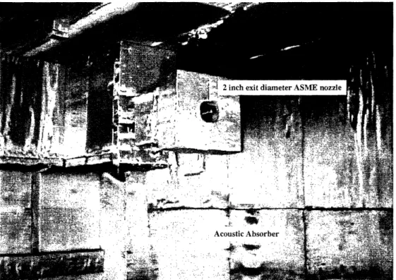
The shock tube is suspended on rollers to provide access to the diaphragms and allow repositioning of the nozzles with respect to the microphones. The nozzles exhaust into an 8.3 m x 9.8 m x 3.7 m anechoic test chamber treated with a 10 cm thick fiberglass acoustic absorber, which results in 10 to 20 dB reduction in reflected acoustic intensity for frequencies above 500 Hz. This precaution is taken to avoid reflection of the jet noise during the test and to eliminate reverberations of the high amplitude noise associated with the initiation of jet flow into the test chamber. The shock tunnel is equipped with a system that flushes the residual helium from the driver section after each test, ensuring subsequent tests are not tainted by extraneous helium. Helium introduced to the test chamber after a test is removed via an exhaust fan located within the test chamber.

(30)

Fluid Jet

Sideline Microphones

R = 4.4 m .

Figure 2-1: MIT shock tunnel facility schematic

Control

Room

7.3 m

(31)

A view of the acoustic chamber and 1/2 0th scale nozzle is shown in Figure, 2-2.

.~~~~~~~~~~-,

', ;.

.

'" :Acoustic Absorber

,

, ~ '

Figure 2-2: View of 1/20th scale ASME nozzle within the acoustic chamber

The control room is shown in Figure 2-3.

Figure 2-3: Shock tunnel facility control room

":. ,..:v - . -. ,

(32)

For a transient facility that acquires only 10-20 ms of data per test to be practical, the turn-around time from test-to-test should be such that 8-10 tests can be completed per day. The run-to-run turn-around time

for this facility was found to be 30-45 minutes depending on the desired set conditions, i.e. the high NPR

condition takes longer to fill the driver section than a low NPR condition.

2.1.2 Test Articles

The primary test articles used in the experiments to assess the performance of the MIT shock tunnel facility are three sizes of ASME standard axis-symmetric nozzles and a Large Scale Model Similitude (LSMS) mixer-ejector model. Furthermore, to compliment the investigation, a series of small exit diameter nozzles were fabricated to fit onto the end of the 1/20h scale ASME nozzle. This section provides a brief description of the nozzle geometries.

2.1.2.1 Small-Scale Nozzles

A series of small scale nozzles, 1/4, Y2, and 3/4 inch exit diameter were fabricated to take advantage of the

compressed air tunnel flushing system. Nozzles of this small size can be run at steady-state as well as under transient conditions to provide an 'in-house' comparison between transient and steady-state acoustic data. A picture of two of the small scale nozzles is shown in Figure 2-4.'

/2 inch exit diameter nozzle I: ,'

,.,

i 1/4 inch exit diameter nozzle

33;..

Figure 2-4: Small-scale round nozzles

The small-scale nozzles are attached to the 5.1 inch exit diameter (1/20th scale) ASME nozzle using three mounting pins located 120 degrees apart, as shown in the figure. Additionally, a bead of silicon is placed around the base of the nozzle to ensure a good seal between the two nozzles.

The dark discoloration shown on the nozzle of Figure 2-4 is black spray-paint that was applied to the nozzle to minimize glare during video diagnostics, which are discussed in Section 6.1.2.1.

(33)

2.1.2.2. ASME Conic Nozzles

The sizes of the three ASME standard. axisymmetric nozzles used on the shock tube to assess facility performance, as well as the ASME nozzle used to acquire steady-state acoustic data, are summarized in Table 2.1.

Table 2.1: Summary of ASME conic nozzle geometry

Nozzle Description I Nozzle Scale I Exit Diameter ] Exit Area, A* I Lp

Transient (Small) 1/20' 2 inches / 5.1 cm 3.14 in2/ 20.43 cm2 7.5 in/ 19.1 cm Transient (Medium) 1/15th

2.67 inches / 6.8 cm 5.6 in2/ 36.32 cm2 10 in / 25.4 cm Transient (Large) 1/1 0th 4 inches / 10.2 cm 12.57 in2/ 81.71 cm2 14 in / 35.6 cm

Steady-State 1/8th 5 inches / 12.7 cm 19.63 in

2

/ 126.67 cm2 17.5 in / 44.5 cm Full-Scale Comparison 1 40 inches / 101.6 cm 1248 in2/ 8051.6 cm2 140 in / 355.6 cm

A picture of the 1/15th Scale ASME nozzle is shown in Figure 2-5a, and the 1/20th mounted on the driven end of the shock tube is shown in Figure 2-5b.

scale ASME nozzle

Figure 2-5: ASME Nozzles (a) 1/1 5th scale ASME conic nozzle, (b) 1/20thscale ASME conic nozzle

mounted on the driven end of the shock tube

2.1.2.3. LSMS Mixer-Ejector Model

The geometry of the LSMS mixer-ejector nozzle is limited rights exclusive (LER), so no explicit definitions of the geometry of the model can be portrayed in this thesis. Figure 1-3 of Chapter 1 provided a conceptual design of a mixer-ejector similar to the one investigated using the shock tunnel. The model is a 1/12'h scale version of the full-size, with an overall length of the model being slightly larger than the 1/10th_{scale ASME nozzle. Figure 2-6 shows the shell of the mixer-ejector, as well as some of the features}

of the model. Figure 2-7 shows a top view of the model, specifically depicting the location of the Kulite pressure transducers. The chute racks tested in the LSMS model are made of either cast aluminum or plastic stereo-lithography, SLA. The aluminum chute rack was cast from an SLA model.

(34)

.Stilling Chamber and/or Secondary Diaphragm Section

ruI I'IUW VI Uil. UllLtll

Figure 2-6: 1/12t scale LSMS model and associated features

Stilling Chamber and/or Secondary Diaphragm Section

Mounting to Driven Section of Shock Tube

Quartz Side-Walls

For Flow Visualization

Figure 2-7: Top view of LSMS model and Kulite pressure transducer locations

Mounting to Driven S of Shock ' 3eometry -ea Ratio A .,UI . YU _ _ V _ . _ _.,,,

(35)

The LSMS model also features an additional five Kulite pressure transducers (9 - 13) located on the bottom of the mixing duct, with transducer number 9 located directly below transducer number 8, and transducer 13 located in the lower bell-mouth assembly. Pressure signatures from these transducers will be shown in Section 4.5. Some digital photos of the LSMS model mounted in the shock tunnel facility are shown in Figures 2-8 - 2-10.

Figure 2-8: Isometric view of LSMS model mounted onto driven section of shock tunnel

(36)

2.1.3 Facility Performance and Range of Operation

The shock tunnel range of performance for the experiments presented in this thesis is summarized in Table 2.2. The shock tube is rated to 100 psi, corresponding to potentially achievable nozzle pressure ratios and total temperature ratios significantly higher than those presented in Table 2.2.

Table 2.2: Summary of shock tunnel facility performance capability

Parameter of Interest Range of Operation

Nozzle Pressure Ratio, NPR 1.5 - 4.0

Total Temperature Ratio, TTR 1.2 - 3.5

Steady-State Nozzle Capability 1/4, 2, and 3/4 inch exit diameters

ASME Nozzles 2, 2.56, and 4 inch exit diameters

Mixer-Ejector Size similar to ASME nozzles

Minimum RmidDe for Steady-State Nozzles 600

Minimum RmiDe for ASME Nozzles 40 (4 inch nozzle, worst case)

Minimum RiJDe for LSMS - 40

Full Scale Frequency Range (B&K 4135) 100 Hz - 8 kHz

Full Scale Frequency Range (B&K 4136) 100 Hz - 6 kHz

Also presented in the summary are the microphone location constraints due to the size of the test chamber (as well as the constraining radius divided by the nozzle exit diameter), and the frequency range which can be measured using the microphones.

2.2 Fluid Mechanic and Acoustic Instrumentation and

Measurement

This section presents an overview of the instrumentation and measurement tools used in the facility to make pressure measurements within the tube and in the test chamber.

2.2.1 Fluid Mechanic and Ambient Condition Measurement Instrumentation

Three Sensotec STJE 0-2000 kPa transducers accurate to ± 690 Pa are mounted in the driver, diaphragm, and driven sections of the shock tube. These transducers are used to display the set pressures of the three sections of the shock tube before each test. Four Kulite XT-190 0-670 kPa dynamic pressure transducers are flush-mounted on the wall of the driven section. These four transducers are used to measure the nozzle pressure, shock speed, and test time (duration of the uniform pressure region). A Paroscientific 0-2000 kPa transducer accurate to + 207 Pa is used to calibrate the Sensotec control and Kulite dynamic pressure transducers. Additionally, two MKS mass flow controllers are employed to control the filling of the driver section of the tube with the helium-air mixture. Ambient conditions are measured just prior to each test

(37)

using a Paroscientific model 740 pressure transducer and Vaisala HMP231 temperature and humidity sensor. Ambient conditions are measured just prior to each test using a Paroscientific model 740 pressure transducer and Vaisala HMP231 temperature and humidity sensor.

2.2.2 Acoustic Instrumentation

This section presents a brief overview of the acoustic instrumentation used in the facility, a description of the microphones and associated support hardware, as well as procedures used to calibrate the microphones.

2.2.2.1 Microphones and Accompanying Support Instrumentation

Acoustic data were acquired using 6 Bruel & Kj.r 4135, 1/4 inch free-field microphones positioned on a

constant radius arc 3.7 m from the nozzle exit at zero degrees incidence; locations are shown in Figure

2-11. I

?

145 deg.

1 140 deg.

,- '

130 deg.

120 deg.

70 deg.

%.% 5~~~~~~~~~~ 110 deg.

Figure 2-11: Microphone locations at constant radius for ASME conic nozzle testing

For an appropriate comparison between the transient and steady-state data, the microphones were located at directivity angles comparable to the steady-state facility. The six microphones were placed at directivity angles: 70, 110, 120, 130, 140, and 145 degrees, as measured- from the inlet axis. To ensure that far-field behavior of the jet noise is captured, the microphones were located at greater than 30 exit diameters away from the nozzle exit. For the 10.2, 6.8 and 5.1 cm exit diameter nozzles, the microphones were located at 39, 57 and 76 exit diameters away, respectively. For the LSMS mixer-ejector model testing the

(38)

microphones were located at slightly different directivity angles2 _{and the microphones were no longer} placed at constant radius to take advantage of room geometry and ease of aziumuthal angle measurement. 3 The microphones used in the experiment are Brulel & Kjer 4135, /4 inch free-field microphones. Some important properties of the B&K 4135 are summarized in Table 2.3.

Table 2.3: Description of B&K 4135 ¼14 inch microphone, [8]

Microphone Property____ Description / Value

Frequency Response Characteristic Free-Field 0°Incidence and Random Incidence

Open Circuit Frequency Response 4 Hz to 100 kHz

Open Circuit Sensitivity mV/Pa 4

Lower Limiting Frequency (-3 dB) 0.3 Hz to 3 Hz

Cartridge Thermal Noise (dB) 29.5

Resonance Frequency 100 kHz

Polarization Voltage 200 V

Condenser microphones require an electric field to be present between the backplate and the diaphragm when being used. The 4135 is an externally polarized microphone that obtains the charge for the electric field from a DC power supply4 connected to the microphone via the preamplifier. Charge build-up on the backplate is not instantaneous, due to the high charge resistance of the preamplifier. Therefore externally polarized microphones reach the correct working voltage after about one minute. Before this time a microphone may not be within specifications. Also, during production, the microphone cartridges are subjected to a high temperature (150 C) forced aging process which ensures long term stability. The predicted long-term stability is of the order of 1 dB over several hundred years at room temperature.

A sample calibration chart for one of the B&K microphones is shown in Figure 2-12. The upper curve is the open circuit free field characteristic, valid for the microphone cartridge without protection grid, for 0°sound incidence. The middle curve is the open circuit random incidence response, valid for the microphone with protection grid DD0023. The lower curve is the open circuit pressure response recorded with an electrostatic actuator. As can be seen from Figure 2-12, the response of the 4135 microphone rapidly rolls-off after around 100 kHz.

2 Peak noise for ASME nozzles is around 130-140 degrees as measured by the convention shown in Figure 2-11. For mixer-ejector tests, the peak noise is expected to be located around 110-120 degrees, hence the microphones for LSMS testing were clustered more tightly around this region.

3 Azimuthal angle geometry is described in Figure 2-19 within Section 2.3. 4 This DC power is provided by the Microphone Multiplexer Type 2822.

(39)

Calibration Chart

ltl-a Cndemr MIaphone

Type 4135 Sarim No 2072162 Callbration Data I:t t: ComatlWa aaam,. K.: COl, CpidU Caibration Condtion Pdadta Voa~

AlMm IltM hPm.U Amnbnl TroPa IRaa H.umily -48.7 m IV/pa ].67 mV/Pa +22.7 dB 6.1 pF 200 V 1 08 hP. 25 'C 50%

Oa.: 02.Jun.1990 SIIaa: 8K

OCbltrlofi dt Vnid at 1013hP, 23'C md 50% RH. For ppu iomal. _ aa awr- d of

1 Pa - N/m' - 1dynr/ans t pbr

I P cralo to i PL 0f 94 dllB 20 pd

dB

-1i

g, 9O 1W 200 W 1o000 2000 5000 10000 20000 0000 OOt00 200000

Figure 2-12: Typical calibration chart for B&K 4135 1/4 inch microphone. SN: 2072162 shown, [9]

When using a free-field response microphone such as the 4135, the microphone should be pointed towards the source. Figure 2-13 shows the free-field corrections for the B&K 4135 microphone with incidence angle. rn 0. 4) C1 -o 'c 0 .2₀₎ 0 0 4 5 6 7 8 910 15 20 30 40 506070 100 Frequency (kHz) 150 200 -801068/1e

Figure 2-13: Free-field corrections for microphones 4135 with protection grid, [8]

4'

..4

I

(40)

For all experiments conducted in this thesis, the microphones were oriented at zero degrees incidence to the source5 and grid caps were left on. The calibration curves shown in figures 2-12 and 2-13 were taken into account in the acoustic data processing, which will be further discussed in Section 2.3:

The microphones are connected to a /2 inch B&K preamplifier Type 2669 using a UA 0035 1/4 to 1/2 inch adapter. The preamplifier has a very high input impedance presenting virtually no load to the

microphone, [9]. The high output voltage, together with an extremely low inherent noise level, gives a wide dynamic range, with a frequency response of ± 0.5 dB between 3 Hz to 200 kHz. The preamplifiers are then connected to cable 2669 B, which in turn connects to B&K Microphone Multiplexer 2822 using a coaxial extension cable AO 0038. The purpose of the multiplexer is to power the pre-amplifiers and to convert the output to a BNC cable which connects to a set of variable gain Pacific amplifiers. From the amplifiers the output is fed into the data acquisition system that is described in Section 2.2.3. A schematic of the microphone assembly and associated support instruments is shown in Figure 2-14.

5m AO 0038 To ADTEK Data 4135 Microphone Type 1669 Coaxial Cable Acqusition System

Cartridge Preamplifier I R(C | I nr Mul Type 2822 xK

111 Multiplexer

UA 0035 2669 B ,,J --_

1/4 to 1/2 Adaptor Connection Cable PacificVariable Gain Amplifer

Figure 2-14: Microphone system schematic and associated components

2.2.2.2 Microphone Calibration

Calibration coefficients for each microphone were obtained with a B&K Pistonphone type 4228 using the procedure described in this section, [11]. The sound pressure level given on the calibration chart for the piston phone is only for the reference conditions stated there. However, ambient conditions will affect the SPL and give rise to a number of corrections. These should, therefore, be taken into account. Ambient condition corrections for pressure, load volume and relative humidity were taken into account during the calibration process to comply with class 1L laboratory requirements, equation 2.1. For improved calibration, a class OL standard should be used, which is presented in equation 2.2.

Class 1L actualSPL = statedSPL + ALp + ALv 2.1

Class OL actualSPL = statedSPL + ALp + AL, + ALH 2.2

5 The source location was taken to be the exit plane of the nozzle. This assumption is further discussed in Chapter 4.