• Aucun résultat trouvé

Bayesian sparse polynomial chaos expansion for global sensitivity analysis

N/A
N/A
Protected

Academic year: 2021

Partager "Bayesian sparse polynomial chaos expansion for global sensitivity analysis"

Copied!
43
0
0

Texte intégral

(1)

HAL Id: hal-01476649

https://hal.archives-ouvertes.fr/hal-01476649

Submitted on 25 Feb 2017

HAL is a multi-disciplinary open access

archive for the deposit and dissemination of sci-entific research documents, whether they are pub-lished or not. The documents may come from

L’archive ouverte pluridisciplinaire HAL, est destinée au dépôt et à la diffusion de documents scientifiques de niveau recherche, publiés ou non, émanant des établissements d’enseignement et de

Bayesian sparse polynomial chaos expansion for global

sensitivity analysis

Qian Shao, Anis Younes, M Fahs, Thierry A. Mara

To cite this version:

Qian Shao, Anis Younes, M Fahs, Thierry A. Mara. Bayesian sparse polynomial chaos expansion for global sensitivity analysis. Computer Methods in Applied Mechanics and Engineering, Elsevier, 2017, 318, pp.474-496. �10.1016/j.cma.2017.01.033�. �hal-01476649�

(2)

Bayesian sparse polynomial chaos expansion for global

sensitivity analysis

Qian Shaoa,b, Anis Younesc,d,e, Marwan Fahsc, Thierry A. Maraa a

PIMENT, EA 4518, Université de La Réunion, FST, 15 Avenue René Cassin, 97715 Saint-Denis, Réunion

b

School of Civil Engineering, Wuhan University, 8 South Road of East Lake, Wuchang, 430072 Wuhan, PR China

c

LHyGeS, UMR-CNRS 7517, Université de Strasbourg/EOST, 1 rue Blessig, 67084 Strasbourg, France

d

IRD UMR LISAH, F-92761 Montpellier, France

e

LMHE, Ecole Nationale d’Ingénieurs de Tunis, Tunisie

Abstract

Polynomial chaos expansions are frequently used by engineers and modellers for uncertainty and sensitivity analyses of computer models. They allow rep-resenting the input/output relations of computer models. Usually only a few terms are really relevant in such a representation. It is a challenge to infer the best sparse polynomial chaos expansion of a given model input/output data set. In the present article, sparse polynomial chaos expansions are in-vestigated for global sensitivity analysis of computer model responses. A new Bayesian approach is proposed to perform this task, based on the Kashyap information criterion for model selection. The efficiency of the proposed al-gorithm is assessed on several benchmarks before applying the alal-gorithm to identify the most relevant inputs of a double-diffusive convection model. keywords: Global sensitivity analysis, Sobol’ indices, Sparse polynomial chaos expansion, Bayesian model averaging, Kashyap information criterion, Double-diffusive convection

email: shaoq88@gmail.com, younes@unistra.fr, fahs@unistra.fr, mara@univ-reunion.frQ. Shao, A. younes, M. Fahs, T.A. Mara (2017), Bayesian sparse polynomial chaos

expansion for global sensitivity analysis, Computer Methods in Applied Mechanics and Engineering, 318, 474–496, doi:10.1016/j.cma.2017.01.033

(3)

Contents

1 Introduction 3

2 Sobol’ decomposition 4

3 Polynomial chaos representation of the model response 6

3.1 Full PC expansion . . . 6

3.2 Computing the PC coefficients . . . 7

3.3 Sparse polynomial chaos expansion . . . 8

3.4 PC-based global sensitivity indices . . . 8

4 The Bayesian Model Averaging Framework 9 5 Bayesian sparse PCE 11 5.1 Our working assumptions . . . 11

5.2 Post-processing . . . 13

5.3 The proposed algorithm . . . 14

6 Synthetic mathematical examples 16 6.1 Ishigami function . . . 16

6.2 Sobol’ function . . . 18

6.3 Morris function . . . 20

7 Application to double diffusive convection in porous media 21 7.1 Problem statement . . . 21

7.2 Sensitivity analysis . . . 23

(4)

1. Introduction

Mathematical models are widely used in many scientific disciplines to explain and understand the observed real world. Their translation into com-puter models allows studying different scenarios by exploring the input space. However, the use of computer models for specific applications is usually ham-pered by the inherent uncertainties about the input values and the model itself. Hence, good modelling practice requires that uncertainties be ac-knowledged and taken into account by modellers. Uncertainty and sensitiv-ity analyses should be routinely implemented both in the modelling process and in the operational use of the model [1].

For this purpose, polynomial chaos expansion (PCE) has received much attention over the last two decades (e.g., [2, 3, 4, 5, 6, 7, 8, 9]). In computer models in engineering, PCE has been proven useful for the analyses of uncer-tainty, sensitivity and risk of failure. A ‘good’ PCE representation contains all the salient features of the model response within the input space in which it has been built. The challenge is to obtain such a ‘good’ representation. There are typically two approaches to building a PCE: intrusive and

non-intrusive. The intrusive approach requires modifying the computer model,

whereas the non-intrusive approach only needs input/output samples. In this paper, we discuss non-intrusive approaches.

The non-intrusive computation of the PCE coefficients is often conducted with one of two methods, projection or regression. The latter is efficient when dealing with a moderate number of input variables. However, with a large number of input variables or a high-degree polynomial, the number of coefficients increases dramatically. In that case, a large number of model evaluations is required to compute the overall set of PCE coefficients (see [7]). Moreover, a large number of coefficients poses the problem of overfitting when regression-based methods are employed. To circumvent this problem, one needs to decrease the number of coefficients in the PCE. To this end, several approaches have been developed to construct a sparse PCE, where only basis functions and coefficients that make significant contributions to the model response of interest are retained. As far as our knowledge extends, the original idea of a sparse PCE came from Blatman and Sudret [10, 11, 12], where they developed an iterative forward–backward algorithm to construct a sparse PCE based on a stepwise regression technique. Later, a least angle regression algorithm was proposed by [13]. Hu and Youn [14] presented a sparse iterative scheme using the projection technique. More recently, Fajraoui et al. [15] developed a simple strategy to construct a sparse PCE from a heuristic rule.

(5)

averag-ing (BMA) is proposed to construct sparse PCEs. BMA, relyaverag-ing on Bayes’ theorem, is a well known statistical approach to perform quantitative com-parisons of competing models [16, 17]. The difficulty of BMA lies in the evaluation of a quantity referred to as the ‘Bayesian model evidence’ (BME), which involves an integral over the whole input space, so it generally has no analytical expression. The Kashyap information criterion (KIC) was derived from BMA under some assumptions regarding the posterior probability dis-tribution [18]. In the present paper, the KIC is employed to select the best sparse PCE for a given input/output sample.

The sparse PCE is employed in the present paper for the global sensitiv-ity analysis of computer model responses. For this purpose, variance-based sensitivity indices are of interest. These sensitivity indices (also called Sobol’ indices) are defined in Section 2. In Section 3, the polynomial chaos rep-resentation of a multi-dimensional function is recalled. In particular, it is given in detail how to determine the Sobol’ indices from the PCE coeffi-cients. Then, in Section 4, the BMA and KIC are defined before proposing, in § 5, our algorithm for inferring the optimal sparse PCE from a given data set. The performance of the proposed algorithm is assessed on different well-known benchmarks for global sensitivity analysis in Section 6. Finally, an application to a porous medium is proposed in Section 7, before concluding (§ 8).

2. Sobol’ decomposition

Let us consider a mathematical model Y =M(X) having an independent input vector X = (X1, . . . , Xn)T and a scalar output Y . We denote by

x= (x1, x2, . . . , xn)T the isoprobabilistic transformed vector of X, namely,

     x1 = F1(X1) .. . xn = Fn(Xn) (1)

where Fi is the cumulative distribution function of Xi, that is, Xi ∼ pi(Xi) =

dFi(Xi)/dXi. Such a transformation is convenient because the input vector

x contains independent random parameters uniformly distributed in the n-dimensional unit hypercube Kn. In the sequel, we assume that Y is square

integrable, that is, Y ∈ L2.

The Sobol’ decomposition represents any square-integrable functionM(X) into a sum of terms of increasing dimensions:

M(X) ≡ M0+ n X i1=1 Mi1(xi1) + n X i2>i1 Mi1i2(xi1, xi2) +· · · + M12...n(x) (2)

(6)

such that Z 1

0 M

i1...is(xi1, . . . , xis)dxik = 0 if k ∈ {1, . . . , s} (3)

On the one hand, Eq. (3) ensures the uniqueness of the decomposition Eq. (2), and on the other hand, ensures the pairwise orthogonality of the summands in the following sense:

Z

KnM

i1...is(xi1, . . . , xis)Mj1...jt(xj1, . . . , xjt)dx = 0

for {i1. . . is} 6= {j1, . . . , jt}

(4)

where dx = dx1. . . dxn for the sake of simplicity.

Moreover, with the above properties, each term in Eq. (2) can be derived analytically. For example, the constant term, the univariate term, and the bivariate terms can be written, respectively, as follows:

M0 = E[M(X)] ≡ Z KnM(X)dx (5) Mi1(xi1) = Z Kn−1M(X)dx∼i 1 − M0 (6) Mi1i2(xi1, xi2) = Z Kn−2M(X)dx∼{i 1,i2}− Mi1(xi1)− Mi2(xi2)− M0 (7) In these expressions, R

Kn−1dx∼i1 denotes the integration over all variables

except xi1. Similarly,

R

Kn−2dx∼{i1,i2} denotes the integration over all

param-eters except xi1 and xi2.

As X is a vector of random variables, the model response Y =M(X) is also a random variable, with variance D:

D = V[M(X)] ≡

Z

KnM

2(X)dx

− M20 (8)

Due to the orthogonality property in Eq. (4), the total variance Eq. (8) can be decomposed as follows: D = n X i1=1 Di1 + n X i2>i1 Di1i2 +· · · + D12...n (9)

where Di1...is is the partial variance:

Di1...is =

Z

KsM 2

(7)

Thereby, the partial sensitivity indices (Sobol’ indices) due to the coopera-tive effect of the input random variables {xi1, . . . , xis} can be defined in the

following form:

Si1...is =

Di1...is

D ∈ [0, 1] (11)

Hence, the first-order sensitivity index Si represents the amount of variance

of the model response due to xi alone. The higher Si, the more Y is sensitive

to the variable xi. Sij measures the amount of variance of Y due to the

co-operative effect (also called the interaction) of xi and xj. To further evaluate

the whole contribution of xi to the variance of Y , the total sensitivity index

ST i is introduced [19]: SiT = X u:i∈u Su (12)

There have been a plethora of methods proposed in the literature to assess the Sobol’ indices. They can be classified as spectral methods [7, 20, 21, 22], non-parametric methods [23, 24, 25, 26], emulator-based methods [27, 28, 29], among others. In the present work, we focus on the spectral method called the polynomial chaos (PC) expansion. In this approach, the model response is cast onto an orthonormal polynomial basis of L2. Thanks to the nature of

the polynomial chaos basis, the sensitivity indices can be computed simply, as analytical functions of the PC coefficients [7].

3. Polynomial chaos representation of the model response

3.1. Full PC expansion

The model response can be expanded as follows in terms of a polynomial basis:

Y =M(X) ≡ X

α∈Nn

aαψα(x) (13)

where α = α1. . . αn (with αi > 0) is an n-dimensional index, and the aα’s

are the PC coefficients.

The multidimensional polynomial ψα1...αn is the tensor product of

uni-variate standardized shifted-Legendre polynomials: ψα1...αn(x) =

n

Y

i=1

ψαi(xi) (14)

We recall that the first shifted standardized Legendre polynomials are: ψ0 =

1, ψ1(x) = √ 3(2x− 1), ψ2(x) = 3 √ 5 2 (2x− 1) 2 √5 2 and so on.

Eq. (13) is usually referred to as the polynomial chaos expansion (PCE) of Y . For computational purposes, the PCE is usually truncated to retain only

(8)

a finite number of terms. One commonly retains those polynomials whose total degree |α| ≡Pn

i=1αi does not exceed a given degree p:

Y ≃ Mp(x)≡ X α∈Ap,n aαψα(x), A p,n ≡ {α ∈ Nn :|α| ≤ p} (15)

With such a truncation, the problem of characterizing the random response Y is reduced to evaluating a finite set of unknown coefficients. The total number of unknown coefficients P can be calculated from the maximal degree p and the number n of input variables as follows:

P =n + p

p 

= (n + p)!

n!p! (16)

where P increases polynomially with both p and n. The expression Eq. (15) is called the full PC representation of degree p of the model response Y .

3.2. Computing the PC coefficients

There are typically two ways to compute the PC coefficients: 1) by projec-tion (see [30] among others) and 2) by regression (e.g., [7]). Projecprojec-tion-based methods exploit the orthonormality of the PC basis elements by assessing the integral

aα=

Z

RnM(X)ψ

α(x)dx (17)

using a numerical integration scheme.

The regression-based methods minimize some distance between the model responses and the truncated PCE,

ap = argmin ap

(L(M(X)|Mp)) (18)

with ap = {aα, 0 6 |α| 6 p} the vector of PC coefficients. L(M(X)|Mp)

defines the distance to be minimized between M and Mp. In a probabilistic

framework, L(·) represents a probability function that measures how likely the identified PCE fits the model response.

With the regression-based methods considered in this paper, a problem arises from the dramatic increase of P when increasing the maximal degree p or the number of input variables n. Indeed, a large number of model evaluations N is required in this context and the evaluation of Eq. (18) can be hampered by overfitting issues. To prevent overfitting, a Bayesian based algorithm is proposed in Section 5 to build a sparse PCE, which retains only a small number of basis functions and PC coefficients to capture the main stochastic features of the model response. Thus, a small number of model evaluations may be sufficient to compute the sparse PC coefficients.

(9)

3.3. Sparse polynomial chaos expansion

LetA be a non-empty finite subset of Nn, with which the truncated PCE

can be defined by

MA(x)≡

X

α∈A

aαψα(x) (19)

The common truncation scheme in Eq. (15) corresponds to the choice A = Ap,n, which is referred to as the full PCE. Since the large cardinality

of this set may lead to the computational issues previously discussed, the determination of truncation sets A of small cardinality is of interest. Thus, we define that if the following condition is verified, the truncated PCE is sparse:

IS = card(A)

card(Ap,n) ≪ 1, p ≡ maxα∈A

(|α|) (20)

In the present paper, a new algorithm, based on Bayesian model selection, is proposed to build sparse PCEs.

3.4. PC-based global sensitivity indices

Once the sparse PCE of a model response is built, a global sensitivity analysis can be carried out at a negligible additional computational cost by analytically computing the Sobol’ indices. Let us consider the PCE in Eq. (19). A subset of multidimensional indices Ii1...is in A is defined such

that Ii1...is =  α∈ A : αk > 0 k∈ (i1, . . . , is), ∀k = 1, . . . , n αk = 0 k /∈ (i1, . . . , is), ∀k = 1, . . . , n  (21) Using this notation, the sparse PCE can be rewritten in the form of the Sobol’ decomposition: MA =a0+ n X i1=1 X α∈Ii1 aαψα(xi1) + n X i2>i1 X α∈Ii1i2 aαψα(xi1, xi2) +· · · + n X is>···>i1 X α∈Ii1,...,is aαψα(xi1. . . , xis) +· · · + X α∈I1,...,n aαψα(x) (22)

where each summand in Eq. (2) can be identified in the above equation as follows: Mi1...is(xi1,...,is) =

P

(10)

Due to the orthonormal property of the polynomial basis, the total and partial variances can be derived analytically from the sparse PCE represen-tation as follows: DA = X α∈A\{0} a2α, D A i1...is = X α∈Ii1...is a2α (23)

Now it is easy to compute the partial sensitivity indices for the subset of input variables {xi1, . . . , xis} from the above equations:

SA i1...is =

DA i1...is

DA (24)

The total sensitivity index of an input variable xi is thus given by the

sum of all the partial sensitivity indices involving i: SiT,A = X

α:αi>0

SαA (25)

In the numerical exercises in Section 6, the estimated sensitivity indices are compared to analytical values for some benchmarks functions. The effi-ciency of the algorithm proposed in Section 5 is assessed by evaluating the following errors with respect to the sample size (i.e., computational cost):

e1 = n X i=1 |Sex i − SiA| (26) eT = n X i=1 |SiT,ex− SiT,A| (27)

where the superscript "ex" stands for the analytical value. 4. The Bayesian Model Averaging Framework

Let us consider Nm plausible competing sparse PCE models MAk:

MAk ≡

X

α∈Ak

aαψα(x), k = 1, . . . , Nm (28)

The above equation can be written in the vector formMAk = akψk with

the parameter vector ak and the vector of polynomial terms ψk. Let X =

{X(1), . . . , X(N )} be a set of input data and Y = {Y(1), . . . , Y(N )}T be the

set of output data such that Y(r) =M(X(r)). The challenge is to scrutinize

(11)

the best sparse PC representation among the set {MAk, k = 1, . . . , Nm}.

To this end, Bayesian model averaging (BMA), a formal statistical approach based on Bayes’ theorem, is introduced to realize an objective ranking and a quantitative comparison of the proposed alternative models. The BMA approach combines prior information of each model with the observed data to estimate the posterior probability for each individual model to be the best one among the competing models. The posterior probabilities P(MAk|Y)

are given by Bayes’ theorem: P(MAk|Y) =

P(Y|MAk)P(MAk)

PNm

i=1P(Y|MAi)P(MAi)

(29) whereP(MAk) is the prior probability that model MAk is the best one from

the set of considered models before any data is collected. The equally likely prior P(MAk) = 1/Nm is usually used if the prior information is vague.

P(Y|MAk) is the likelihood of the observed data, expressing the preference

shown by the data for different models. The denominator in Eq. (29) is the normalization constant, which ensures that the posterior distribution on the left-hand side is a valid probability density and integrates to one. Neglecting the normalizing constant, Bayes’ theorem can be written in the following way:

P(MAk|Y) ∝ P(Y|MAk)P(MAk) (30)

Therefore the key to obtaining the posterior probability is to define the term P(Y|MAk), which is known as the Bayesian model evidence (BME).

This term quantifies the likelihood of the observed data integrated over each model’s parameter space with the following expression:

P(Y|MAk) =

Z

RPk P(Y|MAk

, ak)P(ak|MAk)dak (31)

where Pk is the number of parameters for the model MAk. P(ak|MAk)

denotes the prior distribution of the parameter set ak. P(Y|MAk, ak) is the

likelihood function, which expresses how probable is the observed data for different settings of the parameter vector ak of the model MAk.

The integral in Eq. (31) over the full parameter space of the model is not easy to calculate analytically, especially for high-dimensional parame-ter spaces. A mathematical approximation, e.g., a Taylor series expansion followed by a Laplace approximation is thus used to render the integration computationally tractable. The Laplace approximation assumes that the pos-terior distribution of the parameters is Gaussian and highly peaked around its local maximum with the expression P(ak|Y, MAk) ∼ N (˜ak, C˜a˜a). The

(12)

(MAP), which represents the most likely parameter set for model MAk,

con-sidering both the prior belief about the parameters and the fitting of the observed data. The covariance matrix C˜a˜a is estimated at the MAP solution

(i.e., ak = ˜ak).

Conducting a Taylor expansion of lnP(Y|MAk) centred on the posterior

mode ˜ak, with third- and higher-order terms neglected, then taking the

ex-ponential of the resulting expansion and computing the integration with the Laplace approximation yields

P(Y|MAk)≃ P(Y|MAk, ˜ak)P(˜ak|MAk)(2π)

Pk/2|Σ˜|−1/2 (32)

where ˜Σis the Pk× Pk Hessian matrix of second derivatives of the negative log posterior defined by

h ˜Σi ij =− ∂2lnP(˜a k|Y, MAk) ∂ai∂aj ak=˜ak (33) Eq. (32) yields −2 ln P(Y|MAk)≃ −2 ln P(Y|MAk, ˜ak)−2 ln P(˜ak|MAk)−Pkln(2π)+ln| ˜ Σ| (34) By assuming that the posterior distribution is virtually Gaussian around the MAP (Laplace approximation), one can set ˜Σ= C−1

˜

a˜a, which leads to the

Kashyap information criterion (KIC, [18]):

KICk =−2 ln P(Y|MAk, ˜ak)− 2 ln P(˜ak|MAk)− Pkln(2π)− ln |C˜a˜a| (35)

Evaluating KICk is a computationally feasible alternative to directly

computing BME. KICk reduces the computational effort by considering the

most likely parameter set instead of integrating over the entire parameter space. Note that ˜ak and C˜a˜a in Eq. (35) are usually estimated by

optimiza-tion algorithms.

5. Bayesian sparse PCE

5.1. Our working assumptions

Evaluating the KICk of each competing model MAk allows finding the

best model, the one corresponding to the smallest KIC. Let us define the degree and the interaction order of any index α respectively as follows:

pα≡ |α| = n X i=1 αi, qα ≡ n X i=1 1α i>0 (36)

(13)

where 1αi>0 = 1 if αi > 0 and 0 otherwise.

Moreover, let y = (Y − E [Y ])/V [Y ] be the standardized model response variable and y the vector of standardized model responses. Our strategy to build a sparse PCE for y relies on the first assumption that the model error,

ǫk= y− MAk(x) (37)

is a homoscedastic Gaussian variable, that is, ǫk ∼ N (0, σ2k). This leads to a

Gaussian likelihood function P(Y|MAk, ak, σ 2

k)∼ N (MAk, σ 2

k). The matrix

formulation of the previous equation also becomes

ǫk= y− ψkak (38)

Because MAk is an approximation of y (centred and reduced), it is

ex-pected that the PCE coefficients are close to zero. Consequently, we further assume that P(ak|MAk)∼ N (0, Caa) (39) with Caa =       σ2 α1 0 . . . . 0 . .. 0 . . . ... 0 . .. 0 0 . . . 0 σ2 αPk       where σ2

αi = (pαi + qαi − 1)q2αi stands for the variance assigned to the ith

term in Ak. This prior assigns a high variance to the PC element with a

high level of interactions and a high polynomial degree. This has the effect of favouring low degree and interaction terms by assigning smaller weights to those elements. Note that because y is a standardized vector, a0 is always

equal to zero. Thus, in the following, it is supposed that a0 ∈ A/ k. In the

present work, Gaussian priors are assigned to the PCE coefficients but it is worth mentioning that Laplace priors can also be a good choice [31, 32]. Finally, it is worth mentioning that, except for the model selection criterion, our proposed approach is equivalent to the ridge regression approach [33] and that assuming Laplace priors is tantamount to the Least Absolute Shrinkage and Selection Operator approach (LASSO, see [34]).

By noting that the PCE is linear with respect to its coefficients, the analytical expression of the posterior distribution is given by

P(ak|y, MAk, ˜σ 2

(14)

and P(σk−2|y, MAk, ˜ak)∼ Γ  N + 2 2 , 2 Nσ˜ −2 k  (41) with ˜ ak = Ca˜˜aψTky ˜ σ2 k (42) C˜a = ψ T kψk ˜ σ2 k + C−1 aa −1 (43) ˜ σ2k= (y− ψka˜k) T (y− ψka˜k) N (44)

Eq. (44) gives the MAP estimate of the current model error σ2

k. Solving

Eqs. (42–44) requires an iterative process that starts by setting ˜σ2

k (say, ˜σ2k=

1). Then, after inferring ˜akand C˜a˜a from Eq. (42) and Eq. (43) respectively,

˜ σ2

k is updated from Eq. (44). The calculations are repeated until ˜σk2converges

within a given relative precision (say 10−2). In this context, we can take

advantage of these analytical expressions to evaluate KICk and infer the

best sparse PCE for y. In the sequel, the Bayesian sparse PCE is denoted by MA, and the associated vector of coefficients and the optimal error variance

are denoted by, respectively, aA and σ2

A. Similarly, the PCE degree and level

of interaction are denoted pA and qA, respectively, while PA corresponds to the number of coefficients in the sparse PCE.

5.2. Post-processing

Eqs. (40–41) indicate that aA and σ2

A are random variables.

Conse-quently, the Sobol’ indices estimated with the best sparse PCE should also be treated like random variables as well as any statistics computed with MA. Hence, it is possible to assign a credible interval to the Sobol’ indices

estimate. This is achieved by randomly sampling draws of aA and σ2 A

ac-cording to their posterior densities and evaluating the total variance and partial variances (from Eq. (23)) for each draw before estimating the Sobol’ indices (Eq. (24)). In this way, one obtains a sample of sensitivity indices from which, for instance, the 95% credible interval of each statistic can be extracted. In the sequel, Latin hypercube samples of size 100,000 are gen-erated to evaluate the credible intervals. It is worth mentioning that these calculations are computationally cheap with sparse PCEs.

Since KIC-based PCE selection is a compromise between model simplic-ity and goodness of fit, overfitting is avoided. Thereby one can rely on the relative training error to gauge whether the identified sparse PCE is an ac-curate or poor representation of the original model M. Because the vector

(15)

of model responses is standardized, the relative training error is nothing but σ2

A. However, the validity of this statement relies on the assumption that

the model error is Gaussian, which is not always true. One can confirm this assumption by checking whether the residual (i.e., the vector of model error at the MAP) follows the expected distribution, namely,N (0, σ2

A). If it is not

the case, it is likely that the identified sparse PCE is not reliable. In this situation, it is recommended to increase the sample size where the Laplace approximation is more likely to hold [17].

5.3. The proposed algorithm

Suppose that we have generated an experimental design X = {X(1), . . . ,

X(N )} with N realizations, e.g., a random design based on Monte Carlo

sam-pling, Latin Hypercube sampling or quasi-random low discrepancy sequences. The quasi-Monte Carlo (QMC) method of [35] is adopted for generating sam-ples in this work due to its space filling property. After running the model at the design points, the model responses of interest are gathered into the vector Y = {Y(1), . . . , Y(N )}T. Using the concept of BMA, it is now possible

to devise an algorithm that selects the optimal sparse PCE model from the data set (X , Y). The algorithm is outlined in the following:

Step 1 (Initialization): The data (X , Y) are transformed into standard-ized vectors (x, y). Then, the initial degree and interaction order of the PCE are defined; it is recommended to choose either (p = 2, q = 1) or (p = 4, q = 2), depending on the features of the model response of interest. Further, the following subset is created: Ap,q={α ∈ Nn : p

α 6p, qα 6q}/{0}.

Step 2 (Ranking via correlation coefficient): Set P = Card (Ap,q) and

define the polynomial basis functions ψ = (ψ1, ψ2, . . . , ψP) associated to

Ap,q. Then, calculate the Pearson correlation coefficient r

j between each

polynomial term ψj(x) ∀j = 1, . . . , P and the model response vector y as

follows:

rj =

COV[y, ψj(x)] pV[y]V[ψj(x)]

(45) where COV is the covariance operator. Then, sort the array (r2

1, r22, . . . , r2P)

in descending order and rearrange the polynomial basis functions accordingly in a new vector ˆψ= ( ˆψ1, . . . , ˆψj, ˆψj+1, . . . , ˆψP) such that rj2 >r2j+1.

Step 3 (Ranking via partial correlation coefficient): Compute the partial

correlation coefficient ˆrj|1,...,j−1 between each basis function ˆψj(x) and y for

j = 1, . . . , P with the following equation: ˆ rj|1,...,j−1= COVhy, ˆψj(x)| ˆψ1(x), . . . , ˆψj−1(x)i r Vhy| ˆψ1(x), . . . , ˆψ j−1(x) i Vh ˆψj(x)| ˆψ1(x), . . . , ˆψ j−1(x) i (46)

(16)

where COV [·|·] is the conditional covariance operator and V [·|·] the con-ditional variance operator. As in step 2, sort the array (ˆr2

1, ˆr2|12 , ˆr23|1,2, . . . ,

ˆ r2

P |1,...,P −1) in descending order, based on which we update the vector of PC

basis elements ˜ψ= ( ˜ψ1, . . . , ˜ψj, ˜ψj+1, . . . , ˜ψP) such that ˆrj|1,...,j−12 >rˆj+1|1,...,j2 .

Initialize KIC1 = +∞, ψA= ˜ψ1 and k = 2.

Step 4 (Identification of the current sparse PCE): Define a sparse PCE

model MAk with the polynomial basis ψk = (ψA, ˜ψk). The BMA approach

is used to estimate the current sparse PCE model MAk. Evaluate the MAP estimates ˜ak and Ca˜˜a from Eqs. (42–43) as well as the KICk assigned to

the current model MAk (Eq. (35)). If KICk 6 KICk−1, set ψA = ψk and

aA = ˜ak, otherwise set KICk = KICk−1. Then, set k = k + 1 and repeat

this step until k = P .

Step 5 (Enriching Ap,q): Write M

A = aAψA for the identified sparse

PCE whose elements belongs to the subset A. If the subset A contains (i) elements of degree p− 1 or p, then set p = p + 2 or (ii) elements of level of interaction q, then set q = q + 1 and resume from Step 2 after setting Ap,q = A and enriching the subset from elements of degree p − 1 and p as

well as elements of level of interaction q. Otherwise, stop the calculation. The algorithm starts by considering all the PC basis elements of low degree (typically p = 2) and low level of interactions (q = 1). This ensures that the initial number of elements to be analyzed with the KIC is small. Before evaluating the latter, the basis elements are reordered by order of importance in the next two following steps. First, in Step 2, the Pearson correlation coefficient rj between the model response y and each basis element

ψj is computed. The Pearson correlation coefficient measures the strength of

the linear relation between ψj and y. Consequently, r2j measures how ψj is

a relevant basis element for the investigated sparse PCE. Because there may have been spurious correlations in the experimental design X , the Pearson correlation coefficients can be misleading in highlighting the relevant terms. Consequently, a second reordering is performed in Step 3 on the basis of the estimated partial correlation coefficients. Step 4 proceeds to the identification of the optimal sparse PCE for the basis elements belonging to the current subset Ap,q. Then, the latter is enriched in Step 5 if the optimal sparse PCE

contains elements of degree exceeding p− 1 or level of interactions q. The enrichment is made using basis elements of higher degrees (p + 1, p + 2) and higher levels of interactions (q + 1). In this case, the procedure is resumed for the new subset (from Step 2). If the current identified sparse PCE does not contain basis elements of degree exceeding p− 1 or level interaction q, then the current sparse PCE is deemed the Bayesian sparse PCE MA.

(17)

possible interaction levels q + 1 in Step 5 can provide a very high number of terms in Ap,q. Consequently, during this phase, only the interactions that

involve the relevant inputs of the current iteration are considered. If we consider the multi-dimensional index α = α1. . . αn, the relevant inputs are

those with at least one nonzero index in the subset Ap,q. Thus, ∀α ∈ Ap,q,

if αi1 always equals zero, then xi1 is deemed irrelevant and is not further

considered for higher interaction levels.

Although the proposed enrichment strategy reduces the computational cost, it may result in the identification of a sparse PCE with poor perfor-mance. The quality of the identified PCE modelMAis measured a posteriori

by assessing the relative training error σ2

A. Our experience suggests that a

good sparse PCE satisfies σ2

A < 0.05. Otherwise, it is recommended to restart

the PCE identification procedure with higher initial values of p and q. If the identified PCE is still not satisfactory, then the experimental designX should be enriched and the model response vector Y updated before restarting the identification of the optimal sparse PCE.

Regarding the parameter estimation, we assume that the prior parame-ter and error distributions are both Gaussian. Thus the parameparame-ters can be estimated by the analytical expression of the MAP as described in Section 4. Generally, calculating the MAP analytically allows avoiding the prob-lem of a poorly conditioned matrix usually encountered with the regression method for small sample sizes. However, a larger data set basically yields a more accurate estimation of the sparse PCE, as the Laplace approximation is expected to hold in situations where a relatively large sample size is available. 6. Synthetic mathematical examples

6.1. Ishigami function

Let us consider a popular benchmark in global sensitivity analysis, the Ishigami function [36, 37]:

Y = sin X1+ a sin2X2+ bX34sin X1 (47)

where the inputs are independent random variables uniformly distributed over [−π, π]. This function is smooth, nonlinear and non-monotonic. We note that xi = Xi+12. The total and partial variances of Y can be calculated

analytically: D = a 2 8 + bπ4 5 + b2π8 18 + 1 2, D1 = bπ4 5 + b2π8 50 + 1 2, D2 = a2 8 , D3 = 0,

(18)

D12= D23= 0, D13 =

8b2π8

225 , D123 = 0.

The coefficients in the function take the numerical values a = 7, b = 0.1. Note that the function is sparse in nature since there are three independent variables in the model but the maximum interaction order is 2. Moreover, the function is even with respect to the variables X2 and X3, hence the odd

polynomials of these variables should be zero in the PCE. This means that to identify a good sparse PCE for this function, one must initialize p = 4 and q = 2. Indeed, choosing p = 2 and q = 1 will discard the input variable X3

in the investigated sparse PCE (see the discussion in the previous section). The sparse PCE coefficients are evaluated using quasi-random sequences of different sizes N = 2j(j = 5, 6, . . . , 13). These sequences are used to study

the convergence of the proposed algorithm for building a sparse PCE. The degree and interaction level of the PCE are iteratively increased from p = 4 and q = 2 as described in Section 5.3. The obtained results from the sparse PCEs are reported in Table 1.

Table 1 reveals that N = 26 model evaluations are sufficient to obtain

relatively accurate estimates with a sparse PCE. We note that the relative training error is very small, σ2

A ≃ 1.2 × 10⁻³. The sensitivity indices in this

case show a discrepancy around 2% with respect to the reference solution. With N = 26 model evaluations, the sparse PCE produced by the iterative

procedure has a maximum degree pA = 9 but contains only PA = 13 terms,

whereas the corresponding full PCE would contain P = 3 + 9

9 

= 220 terms (the index of sparsity IS = 13/220 ≈ 0.059) and would thus require at least 220 model evaluations to compute the whole set of coefficients.

Now let us investigate the sensitivity of the sparse PCE estimation to the number of model evaluations. In Table 1 it is observed that the accuracy of the estimates increases with the number of model evaluations. For instance, using N = 25 model evaluations leads to a quite large relative error (σ2

A ≃

0.31) while the latter reduces from N = 26 model evaluations. In particular, a

two-digit accuracy is obtained for all the sensitivity indices for N = 2j, j > 7.

It is also observed that all the sparse PCEs contain relatively low numbers of terms compared to their full counterparts (with indices of sparsity that range from 2.6% to 6.0%), which reflect the sparse structure of the model response.

The various 95% credible intervals of both the first-order and total sensi-tivity indices estimates are plotted in Figure 1 together with the analytical reference values. From this figure, it clearly appears that the credible inter-vals obtained from N = 26 model runs are quite narrow and well centred

(19)

estimates.

Furthermore, the rate of convergence of the proposed procedure for build-ing a sparse PCE is studied. In Figure 2, the absolute errors of the first-order and total sensitivity indices are reported as functions of the number of model evaluations. The results of this figure show a high convergence rate of the sensitivity indices with respect to the number of model evaluations for the sparse PCE. This high convergence rate is due to the smoothness of the Ishigami function.

All the statistics computed with the identified Bayesian sparse PCEs for different sample sizes are reliable under the assumption of Gaussian model errors. To check this assumption a posteriori, the empirical cumulative dis-tribution function (CDF) of the residual evaluated at the MAP is compared with the expected normal CDF. This comparison is carried out for different sample sizes (see Figure 3). It can be inferred that, except for N = 25, the

residuals are virtually normally distributed. Hence, assuming a Gaussian error between the Ishigami function and the Bayesian sparse PCE seems a reasonable assumption.

To test the stability of the algorithm, for different sample sizes we re-peat one hundred times the Bayesian sparse PCE identification from different draws. To do so, the quasi-random sequences are generated by sampling from different points in the input space. The results are depicted in Figure 4 in the form of box-and-whisker plots. The latter show relatively large variations of the Sobol’ indices estimates, especially at low sample sizes (N = 25, 26). We

note that, as compared to the uncertainty ranges provided by the Bayesian sparse PCE (see Figure 1), the effect of the experimental design is non-negligible at low sample sizes. Thereby, the uncertainties computed with the optimal sparse PCE are underestimated. To obtain more reliable uncertain-ties one could consider all probable sparse PCEs instead of considering only the best one. We did not consider this alternative in the present work.

6.2. Sobol’ function

Let us consider the Sobol’ function [23]: Y = n Y i=1 |4Xi− 2| + bi 1 + bi (48) where the input variables Xi, i = 1, . . . , n are uniformly distributed over [0, 1].

This function is non-smooth and non-monotonic. The analytical expressions of the total and partial variances are

D = n Y i=1 (Di+ 1)− 1, Di = 1 3(1 + bi)2 , Di1...is = s Y k=1 Dik.

(20)

For numerical application, we set the number of input variables n = 9 and bi = (i− 1)/4. This function is a challenging one due to the presence of the

absolute value which slows down the convergence of the PCE. Moreover, the level of interactions is very high, as revealed by the differences between the first-order and total Sobol’ indices (see Table 2, column #2).

For the same reason as before, the initial degree and interaction order of the sparse PCE are p = 4 and q = 2. Several sample sizes are used to assess the efficiency of the algorithm N = 2j, (j = 5, . . . , 13). Inaccurate results were obtained for sample sizes less than N = 28. The results are listed in

Table 2 for N = 28, . . . , 213 and depicted in Figure 5.

It can be observed that with the increase of the number of model eval-uations, the accuracy of the Bayesian sparse PCE slightly improves. The relative training error σ2

A never decreases below 10−2 (see the last row of

Table 2). With N = 212 model evaluations, the sparse PCE yields estimates

with an accuracy similar to the reference solution (discrepancy less than 8%). In this case, the sparse PCE has a maximum degree pA = 18 and total terms PA = 174, revealing a noticeably small sparsity index of 3.7× 10⁻⁵ with

re-spect to a full PCE of the same degree. Indeed, the corresponding full PCE of degree p = 18 would contain P = 4, 686, 825 terms. This would be com-putationally unaffordable because of the large number of model evaluations required.

The credible intervals assigned to the estimated sensitivity indices are depicted in Figure 5. The uncertainty bounds are particularly large at low sample sizes and become very narrow from N > 211. Yet, despite of the

rel-atively large uncertainties at N = 28 and N = 29, the first three inputs are

identified as significantly more important than the remainder. Surprisingly, for N = 210 the subset of inputs (x

3, x4, x5) is found of equal importance.

Although at N = 211 the uncertainties assigned to the estimated total

sensi-tivity indices are very narrow, they do not encompass the analytical values (meaning that the estimated values are slightly biased). This indicates that the proposed approach may require a lot of model runs to accurately capture the structure of non-smooth functions.

Figure 6 shows the rate of convergence of the proposed procedure for building a sparse PCE in terms of the absolute errors of the first-order and total sensitivity indices as functions of the number of model evaluations. The results show that the convergence rate of the proposed method for the Sobol’ function is relatively slow compared to the results for the Ishigami function. This low convergence rate is due to the loss of the spectral convergence of the PCE for non-smooth functions.

The Gaussian error assumption is checked a posteriori by comparing the CDF of the residual with the expected target CDF (see Figure 7). It can

(21)

be noted that, albeit some slight discrepancies, the CDFs match surprisingly well despite the non-smoothness of the Sobol’ function. Hence, it can be concluded that the Gaussian error assumption is acceptable in the present exercise.

The stability of the algorithm is again tested by replicating one hundred times the Bayesian sparse PCE identification at different sample sizes. The results are depicted in Figure 8. We note that the total sensitivity indices estimates are more sensitive to the experimental design (bottom plot) than the first-order sensitivity indices (top plot). The influence of the experimental design at low sample sizes is very important on the uncertainty range and on the bias. They decrease with the increase of the sample size.

6.3. Morris function

To assess the proposed method for large dimensional problems, we con-sider now the so-called Morris function [38]:

Y = β0+ 20 X i=1 βiXi+ 20 X i<j βijXiXj+ 20 X i<j<k βijkXiXjXk+ 20 X i<j<k<l βijklXiXjXkXl (49) where Xi = 2(1.1xi/(xi+ 0.1)− 0.5) if i = 3, 5, 7 2(xi − 0.5) otherwise (50)

and the xis are uniformly distributed over [0,1]. The coefficients βi are

as-signed as follows:        βi = 20 for i = 1, . . . , 10 βij =−15 for i, j = 1, . . . , 6 βijk =−10 for i, j, k = 1, . . . , 5 βijkl = 5 for i, j, k, l = 1, . . . , 4 (51)

The remaining coefficients are zero.

The sensitivity indices are computed by post-processing the sparse PCE obtained by setting the initial degree and interaction order to p = 2 and q = 1. This choice is reasonable because, unlike the previous cases, the Morris function is neither even nor odd, and its dimensionality is high. Hence, initializing p = 2 and q = 1 allows reducing the computational time of the postprocessing. Different sizes of experimental designs N = 2j, (j =

5, 6, . . . , 13) are used to build the sparse PCE. Because there are no reference values for this function, we assess the quality of the estimation by comparing the sensitivity indices and their credible intervals.

(22)

Figure 9 shows the ten greatest total sensitivity indices with their un-certainty bounds for the different sample sizes. It is found that the credible intervals with a small number of model evaluations (N = 25 and N = 27)

are relatively wide, which indicates the necessity of enlarging the number of model evaluations to get more accurate results. Much narrower uncertainty bounds are found using large numbers of model evaluations (N = 29, 211 and

213) in Figure 9. The values of the total sensitivity indices are greater than

those of the first-order sensitivity indices, which demonstrates that the model is non-additive and contains interactions between the parameters. Moreover, we can observe in Figure 9 that ST

1, S2T and S4T are the three greatest values

and have almost the same importance. ST

3, S5T, S6T, S8T, S9T and S10T have

in-termediate values. From the sample size N = 29, the following classification

of the input variables can be made:

• a group of important variables: x1, x2, x4;

• variables with intermediate significance: x3, x5, x6, x8-x10;

• one variable with small importance: x7;

• a group of non-significant variables: x11-x20.

7. Application to double diffusive convection in porous media

7.1. Problem statement

In this section, the methodology developed for sensitivity analysis is ap-plied to the problem of double diffusive convection (DDC) in saturated porous media. DDC occurs when the saturating fluid contains several constituents and when the density gradients inducing natural convection are caused simul-taneously by the temperature and compositional effects. This configuration has received considerable attention in recent years due to the wide range of its environmental and energetic applications. DDC in porous media involves multiple physical processes related to the flow, heat transfer, mass transfer, and buoyancy forces. For this reason, it is an appropriate concrete problem for testing new methods of sensitivity analysis.

The problem under consideration is that of a square porous cavity with horizontal mass and thermal gradients (Figure 10). The left and right vertical walls of the cavity are subjected to normalized temperatures and concentra-tions TL = CL = 1 and TR = CR = 0, respectively. The horizontal surfaces

are assumed to be adiabatic and impermeable. The heat and mass gradients generate buoyancy forces and yield to a rotating unit cell within the cavity. This problem has played a key role in the investigation of the DDC in porous

(23)

media. However, as far as our knowledge extends, no global sensitivity anal-ysis has ever been conducted to identify the most relevant model inputs for DDC.

To model DDC in porous media, the fluid flow in the cavity is assumed to comply with Darcy’s law and the Boussinesq approximation. The porous medium is in local thermal equilibrium with the fluid. Under these condi-tions, the steady state governing equations of the fluid flow as well as the heat and mass transfer inside the porous cavity can be written in the following non-dimensional form: ∂u ∂x + ∂v ∂y = 0 (52) H2 K u =− ∂pt ∂x (53) H2 K v =− ∂pt ∂y + GrT (T + Nr.C) (54) u∂T ∂x + v ∂T ∂y = Rk P r  ∂2T ∂x2 + ∂2T ∂y2  (55) u∂C ∂x + v ∂C ∂y = 1 Le.P r  ∂2C ∂x2 + ∂2C ∂y2  (56) where H is the size of the square cavity, u and v are the velocity components in the x ∈ [0, 1] and y ∈ [0, 1] directions, pt is the total pressure of the

system including the fluid pressure and gravitational head, T and C are the temperature and concentration, respectively, Rk is the ratio of the effective

thermal diffusivity of the porous medium to that of the fluid, P r, Le and GrT

are the Prandtl, Lewis and thermal Grashof numbers, respectively, Nr is the buoyancy ratio, and K is the permeability of the stratified porous medium, defined by

K(x, y) = K0eζ1Hx+ζ2Hy (57)

Here, K0 is the permeability at the origin, while ζ1 and ζ2 are the rates of

change of ln(K) in the x and y directions. In the simulation, the average permeability and Rayleigh number are defined for the heterogeneous porous medium as follows: K = Z 1 0 Z 1 0 K(x, y)dxdy (58) Ra = K.P r.GrT H2 (59)

The system is solved using the highly accurate Fourier–Galerkin (FG) method described in [39, 40]. The FG method is one of the most popular

(24)

spectral methods, used extensively in large-scale computations to solve par-tial differenpar-tial equations because of its ability to achieve high precision with a relatively small number of degrees of freedom. The method consists in expanding the unknowns (stream function, temperature and concentration) into the appropriate Fourier series truncated at given orders. As shown in [40], the number of Fourier modes required to obtain stable solutions with the FG method depends on the average Rayleigh number (Ra) and the level of heterogeneity (ζ1 and ζ2). In this paper, the sensitivity analysis requires

several evaluations of the model. Hence, moderate ranges of Ra and (ζ1, ζ2)

are used in order to obtain accurate solutions in an affordable CPU time (see Table 3). The level of truncation orders of the Fourier series is fixed to be 90 and 30 in the x and y directions, respectively. Thus a total number of 3× 90 × 30 = 8100 Fourier coefficients are determined in the computation.

The model parameters are listed in Table 3. The size of the cavity H and the ratio of thermal diffusivity Rk are considered as deterministic. The

Prandtl number, the average Rayleigh number, the average permeability, the rates of change of the permeability in the x and y directions, the Lewis num-ber, and the buoyancy ratio are assumed to be random parameters. Their properties are specified in Table 3. These parameters are gathered into a random vector X = (P r, Ra, K, ζ1, ζ2, Le, Nr)T of dimension n = 7. All

seven random variables are supposed to be uniformly and independently dis-tributed.

The model responses of interest are the average Nusselt and Sherwood numbers (Nu, Sh), as well as the maximum velocity components (umax, vmax)

in the x and y directions. These variables are commonly used to investigate DDC problems because they provide a quantitative idea of the fluid circu-lation velocity, as well as the heat and mass fluxes. The average Nusselt number (resp. Sherwood number) represents the ratio of the total rate of heat transfer (resp. mass transfer) to the rate of conductive heat transfer (resp. diffusive mass transport) across the boundary. They are defined by

Nu = Z 1 0 ∂T ∂x x=0 dy (60) Sh = Z 1 0 ∂C ∂x x=0 dy (61) 7.2. Sensitivity analysis

The sensitivity indices of the input parameters (P r, Ra, K, ζ1, ζ2, Le, Nr)

are estimated using the Bayesian sparse PCE approach. The initial size of the quasi-random experimental design is N = 25. The experimental design is

pro-gressively enriched until a satisfactory solution is reached (σ2

(25)

In this example, a satisfactory sparse PCE is obtained with a sample size of N = 27, for which we found σ2

A(Nu) = 3.1× 10⁻³, σ2A(Sh) = 3.9× 10⁻³,

σ2

A(umax) = 2.1×10⁻², and σA2(vmax) = 1.5×10⁻². The 95% credible interval

of each sensitivity index is derived using the scheme outlined in Section 5.2. The estimates of the first-order and total sensitivity indices are sketched in Figure 11. In this figure, the credible intervals are quite narrow for all the sensitivity indices, which demonstrates the validity of the sparse PCE estimation. It also appears that the variances of the model responses are due to distinct random variables. For instance, for the first model response Nu, the variance is mainly explained by the average Rayleigh number Ra and buoyancy ratio Nr. As a matter of fact, the Nusselt number represents the dimensionless thermal diffusive flux through the hot wall, which is propor-tional to the temperature gradient. The latter is in turn proporpropor-tional to the thickness of the thermal boundary layer generated by the fluid circulation within the porous cavity. The origin of this flow lies in the buoyancy forces, which are mainly controlled by the Rayleigh number and the buoyancy ra-tio for the thermal effects. The same behaviour is noted for the average Sherwood number Sh, which represents the solute diffusive flux at the salted wall. However, for Sh, we can notice the additional influence of the Lewis number Le, which is the main parameter controlling the mass diffusivity. For both Nu and Sh, Figure 11 shows that Ra has the most significant contri-bution. Besides, for both Nu and Sh, the total sensitivity indices are close to the first-order sensitivity indices, which means that the relations between the model responses (Nu, Sh) and the parameters are practically additive (negligible interactions). Regarding the model responses umax and vmax, it is

shown in Figure 11 that the influence of P r and Ra are both significant. This may be explained by the fact that P r and Ra are related to the viscous and buoyancy effects, which play the key roles in the fluid flow process. The total sensitivity indices of P r and Ra are greater than their first-order sensitivity indices, which indicates the existence of interactions between them.

The identified sparse PCEs only contain 13, 15, 16 and 15 terms in the expansions for Nu, Sh, umax, and vmax, respectively, which indicates a high

sparsity. Taking the model response umax, for example, the maximum degree

of the sparse PCE is pA = 6. Thus a full PCE of the same degree would contain P = 10, 296 terms, which yields a sparsity index of 1.5× 10⁻³.

8. Conclusion

In this paper, a new algorithm is proposed to build sparse PCEs of com-puter model responses. They are then used to compute Sobol’ indices for global sensitivity analysis. The new algorithm relies on the statistical

(26)

ap-proach called BMA, which performs quantitative comparisons of competing models. In particular, the model selection criterion KIC is adopted to identify the best sparse PCE from a given data set. We propose a new algorithm to construct a sparse PCE that only contains the significant polynomial terms for the data set at hand. Thus, a reduced number of coefficients is esti-mated. Using the analytical expression of the MAP, the retained coefficients are computed with a low number of model evaluations (as compared to the full PCE), avoiding the problem of a poorly conditioned matrix encountered with the regression method.

The proposed algorithm is tested on four examples of applications, includ-ing three analytical functions, namely the Ishigami function (smooth), the Sobol’ function (non-smooth), and the Morris function (high-dimensional). The fourth example is a Fourier–Galerkin model for double-diffusive con-vection in a heterogeneous porous cavity. High sparsity is found in these examples, with a sparsity index varying from 0% to 6%. Using Bayesian sparse PCE, good estimates of the sensitivity indices can be obtained with a rather low number of model evaluations compared to full PCE.

Moreover, thanks to the Bayesian framework, the posterior distribution of the coefficients in the sparse PCE can be easily computed. Accordingly, it is possible to assign credible interval to each sensitivity index with little computational effort. Furthermore, the accuracy of the sparse PCE is eval-uated by both the residual and the size of the credible intervals. Although our study reveals that these intervals can be underestimated, they allow for gauging the degree of importance of the input variables. The numerical ex-ercises also show that the proposed Bayesian sparse PCE can yield estimates of the sensitivity indices with low bias and variance.

Acknowledgement

This work has been funded by the French National Research Agency through the research project RESAIN (n◦ ANR-12-BS06-0010-02).

References

[1] A. Saltelli, M. Ratto, T. Andres, F. Campolongo, J. Cariboni, D. Gatelli, M. Saisana, S. Tarantola, Global Sensitivity Analysis: The Primer, Probability and Statistics, John Wiley and Sons, Chichester, 2008. [2] R. G. Ghanem, S. P. Spanos, Stochastic finite elements: A spectral

(27)

[3] M. A. Tatang, W. W. Pan, R. G. Prin, G. J. McRae, An efficient method for parametric uncertainty analysis of numerical geophisical model, J. Geophysics Research 102 (1998) 21925–21932.

[4] D. Xiu, G. E. Karniadakis, The Wiener-Askey polynomial chaos for stochastic differential equations, SIAM, Journal of Scientific Computing 24 (2002) 619–644.

[5] O. Le Maître, M. T. Reagan, H. N. Najm, R. G. Ghanem, O. M. Knio, A stochastic projection method for fluid flow: II. Random process, Journal of Computational Physics 181 (9–44).

[6] H. G. Matthies, A. Keese, Galerkin methods for linear and nonlinear elliptic stochastic partial differential equations, Computer Methods in Applied Mechanics & Engineering (2005) 1295–1331.

[7] B. Sudret, Global sensitivity analysis using polynomial chaos expan-sions, Reliability Engineering and System Safety 93 (2008) 964–979. [8] N. Fajraoui, F. Ramasomanana, A. Younes, T. A. Mara, P. Ackerer,

A. Guadagnini, Use of global sensitivity analysis and polynomial chaos expansion for interpretation of nonreactive transport experiments in laboratory-scale porous media, Water Resources Research 47, W02521 (2011) doi:10.1029/2010WR009639.

[9] M. Riva, A. Guadagnini, A. Dell’Oca, Probabilistic assessment of seawa-ter intrusion under multiple sources of uncertainty, Advances in Waseawa-ter Resources 75 (2015) 93–104.

[10] G. Blatman, B. Sudret, Sparse polynomial chaos expansions and adap-tive stochastic finite elements using a regression approach, Comptes Ren-dus de Mécanique 336 (2008) 518–523.

[11] G. Blatman, B. Sudret, Efficient computation of global sensitivity in-dices using sparse polynomial chaos expansions, Reliability Engineering and System Safety 95 (11) (2010) 1216–1229.

[12] G. Blatman, B. Sudret, An adaptive algorithm to build up sparse poly-nomial chaos expansions for stochastic finite element analysis, Proba-bilistic Engineering Mechanics 25 (2010) 183–197.

[13] G. Blatman, B. Sudret, Adaptive sparse polynomial chaos expansion based on least angle regression, Journal of Computational Physics 230 (6) (2011) 2345–2367.

(28)

[14] C. Hu, B. D. Youn, Adaptive-sparse polynomial chaos expansion for reliability and design of complex engineering systems, Structural and Multidisciplinary Optimization 43 (2010) 419–442.

[15] N. Fajraoui, T. A. Mara, A. Younes, R. Bouhlila, Reactive transport parameter estimation and global sensitivity analysis using sparse poly-nomial chaos expansion, Water, Air and Soil Pollution 223 (2012) 4183– 4197.

[16] S. P. Neuman, Maximum likelihood Bayesian averaging of uncertain model predictions, Stochastic Environmental Research and Risk Assess-ment 17 (5) (2003) 291–305.

[17] A. Schöniger, T. Wöhling, L. Samaniego, W. Novak, Model selection on solid ground: Rigourous comparison of nine ways to evaluate Bayesian evidence, Water Resources Research 50 (2014) 9484–9513.

[18] R. L. Kayshap, Optimal choice of AR and MA parts in autoregressive moving average models, IEEE Trans. Pattern Anal. Machine Intell. 4 (2) (1982) 99–104.

[19] T. Homma, A. Saltelli, Importance measures in global sensitivity anal-ysis of nonlinear models, Reliability Engineering and System Safety 52 (1996) 1–17.

[20] R. I. Cukier, C. M. Fortuin, K. E. Shuler, A. G. Petschek, J. H. Schaibly, Study of the sensitivity of coupled reaction systems to uncertainties in rate coefficients. I. theory, J. Chemical Physics 59 (1973) 3873–3878. [21] A. Saltelli, S. Tarantola, K. Chan, A quantitative model independent

method for global sensitivity analysis of model output, Technometrics 41 (1999) 39–56.

[22] T. A. Mara, Extension of the rbd-fast method to the computation of global sensitivity indices, Reliability Engineering and System Safety 94 (2009) 1274–1281.

[23] I. M. Sobol’, Sensitivity estimates for nonlinear mathematical models, Math. Mod. and Comput. Exp. 1 (1993) 407–414.

[24] M. J. J. Jansen, Analysis of variance designs for model output, Computer Physics Communication 117 (1999) 35–43.

[25] A. Saltelli, Making best use of model evaluations to compute sensitivity indices, Computational Physics Communications 145 (2002) 280–297.

(29)

[26] H. Rabitz, O. Alis, J. Shorter, K. Shim, Efficient input-output model representations, Computer Physics Communications 117 (1999) 11–20. [27] J. E. Oakley, A. O’Hagan, Probabilistic sensitivity analysis of complex

models: a Bayesian approach, J. Royal Statist. Soc. B 66 (2004) 751– 769.

[28] M. Ratto, A. Pagano, P. Young, State dependent parameter meta-modelling and sensitivity analysis, Computer Physics Communications 117 (11) (2007) 863–876.

[29] G. T. Buzzard, D. Xiu, Variance-based global sensitivity analysis via sparse-grid interpolation and cubature, Communications in Computa-tional Physics 9 (2011) 542–567.

[30] T. Crestaux, O. L. Maître, J.-M. Martinez, Polynomial chaos expansion for sensitivity analysis, Reliability Engineering and System Safety 94 (2009) 1161–1172.

[31] K. Sargsyan, C. Safta, H. N. Najm, B. J. Debusschere, D. Ricciuto, P. Thornton, Dimensionality reduction for complex models via Bayesian compressive sensing, International Journal for Uncertainty Quantifica-tion (2014) 63–93.

[32] S. D. Babacan, R. Molina, A. K. Katsaggelos, Bayesian compressive sensing using Laplace priors, IEEE Trans. on Image Process. (2010) 53– 63.

[33] A. E. Hoerl, R. Kennerd, Ridge regression: Biased estimation for nonorthogonal problems, Technometrics 12 (1970) 55–67.

[34] R. Tibshirani, Regression shrinkage and selection via the LASSO, Jour-nal of the Royal Statistical Society, Serie B 58 (1) (1996) 267–288. [35] I. M. Sobol’, V. I. Turchaninov, Y. L. Levitan, B. V. Shukman,

Quasi-random sequence generator (routine LPTAU51), Keldysh Institute of Applied Mathematics, Russian Academy of Sciences (1992).

[36] A. Saltelli, K. Chan, E. M. Scott, Sensitivity analysis, John Wiley and Sons, Chichester, 2000.

[37] T. Ishigami, T. Homma, An importance quantification technique in un-certainty analysis for computer models, in: First International Sympo-sium on Uncertainty Modeling and Analysis, IEEE, 1990, pp. 398–403.

(30)

Table 1: Ishigami function—Sensitivity indices estimated with Bayesian sparse PCE versus the number of model runs

Ref. Val. N = 25

N = 26

N = 27

N = 28 Est. Err. (%) Est. Err. (%) Est. Err. (%) Est. Err. (%)

S1 0.31 0.35 12.8 0.31 -1.7 0.31 -0.7 0.31 0.0 S2 0.44 0.65 46.0 0.45 2.2 0.44 0.3 0.44 0.0 S3 0.00 0.00 - 0.00 - 0.00 - 0.00 -ST 1 0.56 0.35 -36.5 0.55 -1.8 0.56 -0.2 0.56 0.0 ST 2 0.44 0.65 46.0 0.45 2.2 0.44 0.2 0.44 0.0 ST 3 0.24 0.00 -100.0 0.24 -1.9 0.24 0.5 0.24 0.0 pA 6 9 9 12 qA 1 2 2 2 PA 5 13 13 17 IS 6.0 × 10⁻² 6.0 × 10⁻² 6.0 × 10⁻² 3.7 × 10⁻² σ2 A 3.1 × 10 −1 1.2 × 10⁻³ 2.1 × 10⁻³ 1.2 × 10⁻⁵ N = 29 N = 210 N = 211 N = 212 N = 213 Est. Err. (%) Est. Err. (%) Est. Err. (%) Est. Err. (%) Est. Err. (%)

0.31 0.0 0.31 0.0 0.31 0.0 0.31 0.0 0.31 0.0 0.44 0.0 0.44 0.0 0.44 0.0 0.44 0.0 0.44 0.0 0.00 - 0.00 - 0.00 - 0.00 - 0.00 -0.56 0.0 0.56 0.0 0.56 0.0 0.56 0.0 0.56 0.0 0.44 0.0 0.44 0.0 0.44 0.0 0.44 0.0 0.44 0.0 0.24 0.0 0.24 0.0 0.24 0.0 0.24 0.0 0.24 0.0 12 14 14 14 16 2 2 2 2 2 20 22 22 22 25 4.4 × 10⁻² 3.2 × 10⁻² 3.2 × 10⁻² 3.2 × 10⁻² 2.6 × 10⁻² 1.9 × 10⁻⁸ 1.5 × 10⁻⁸ 1.5 × 10⁻⁸ 1.5 × 10⁻⁸ 9.0 × 10⁻¹²

[38] M. D. Morris, Factorial sampling plans for preliminary computational experiments, Technometrics 33 (1991) 161–174.

[39] Q. Shao, M. Fahs, A. Younes, A. Makradi, A high-accurate solution for darcy–brinkman double-diffusive convection in saturated porous media, Numerical Heat Transfer, Part B: Fundamentals 69 (2016) 26–47. [40] M. Fahs, A. Younes, A. Makradi, A reference benchmark solution for free

convection in a square cavity filled with a heterogeneous porous medium, Numerical Heat Transfer, Part B: Fundamentals 67 (2015) 437–462.

(31)

Table 2: Sobol’ function—Sensitivity indices estimated with Bayesian sparse PCE versus the number of model runs Ref. Val. N = 28 N = 29 N = 210 N = 211 N = 212 N = 213

Est. Err. (%) Est. Err. (%) Est. Err. (%) Est. Err. (%) Est. Err. (%) Est. Err. (%)

S1 0.19 0.26 33.8 0.21 6.1 0.23 19.0 0.21 8.5 0.20 3.0 0.20 2.1 S2 0.12 0.18 43.4 0.16 26.2 0.16 25.5 0.14 8.4 0.13 3.7 0.13 2.7 S3 0.09 0.13 55.9 0.11 26.7 0.08 -7.3 0.10 10.3 0.09 1.9 0.09 1.7 S4 0.06 0.05 -14.6 0.08 22.5 0.08 33.2 0.07 4.8 0.07 6.8 0.06 1.7 S5 0.05 0.05 5.7 0.05 5.2 0.06 29.6 0.05 9.1 0.05 3.1 0.05 -0.8 S6 0.04 0.02 -53.1 0.03 -22.3 0.04 6.3 0.04 5.2 0.04 7.6 0.04 2.0 S7 0.03 0.03 -14.8 0.03 -3.4 0.03 6.7 0.03 8.7 0.03 4.1 0.03 2.0 S8 0.03 0.02 -3.4 0.03 31.7 0.03 2.1 0.03 10.7 0.03 4.6 0.03 3.5 S9 0.02 0.03 34.5 0.02 -9.2 0.02 6.1 0.02 15.1 0.02 4.5 0.02 2.6 ST 1 0.40 0.41 4.2 0.39 -1.5 0.37 -5.9 0.39 -1.8 0.39 -0.3 0.39 -0.3 ST 2 0.28 0.29 3.6 0.19 4.0 0.29 4.4 0.26 -6.0 0.27 -2.8 0.28 -0.2 ST 3 0.20 0.22 6.1 0.21 4.5 0.15 -28.7 0.20 -2.4 0.19 -5.6 0.20 -2.4 ST 4 0.16 0.07 -56.2 0.17 7.1 0.16 4.3 0.14 -11.7 0.16 0.8 0.15 -2.3 ST 5 0.12 0.10 -20.0 0.08 -30.6 0.14 14.2 0.11 -8.0 0.11 -6.4 0.11 -8.0 ST 6 0.10 0.03 -70.0 0.08 -22.6 0.10 -0.1 0.08 -16.3 0.10 -2.2 0.09 -5.1 ST 7 0.08 0.04 -50.3 0.06 -30.3 0.07 -16.9 0.07 -16.9 0.08 -4.5 0.08 -4.4 ST 8 0.07 0.04 -40.4 0.05 -31.7 0.05 -30.8 0.06 -7.3 0.06 -4.2 0.07 0.0 ST 9 0.06 0.03 -48.6 0.05 -17.5 0.07 27.6 0.05 -5.2 0.05 -6.0 0.06 -2.1 pA 4 8 18 16 18 16 qA 2 4 7 8 8 8 PA 19 30 45 99 174 321 IS 2.7 × 10⁻² 1.2 × 10⁻³ 9.6 × 10⁻⁶ 4.8 × 10⁻⁵ 3.7 × 10⁻⁵ 1.6 × 10⁻⁴ σ2 A 2.1 × 10 −1 1.8 × 10⁻¹ 1.6 × 10⁻¹ 5.8 × 10⁻² 3.3 × 10⁻² 1.9 × 10⁻² 30

(32)

Table 3: Parameters of the double-diffusive convection model

Parameter Notation Type of PDF Range of values

Size of cavity H Deterministic 1.0

Ratio of thermal diffusivity Rk Deterministic 1.0

Prandtl number P r Uniform [0.5, 2.0]

Average Rayleigh number Ra Uniform [1.0, 100.0]

Average permeability K Uniform [10−9

, 10−7 ] Rate of change in x direction ζ1 Uniform [0.0, 2.0] Rate of change y direction ζ2 Uniform [0.0, 2.0]

Lewis number Le Uniform [1.0, 5.0]

(33)

Figure 1: Ishigami function—95% confidence intervals of the first-order and total sen-sitivity indices computed from Bayesian sparse PCE with different numbers of model evaluations

(34)

Figure 2: Ishigami function—Absolute errors of first-order and total sensitivity indices computed as functions of the number of model evaluations

(35)

-1.5 -1 -0.5 0 0.5 1 1.5 2 0 0.5 1 C D F N = 25 Empirical Target -0.2 -0.1 0 0.1 0.2 0 0.5 1 N = 2 6 -0.2 -0.1 0 0.1 0.2 0 0.5 1 C D F N = 27 -0.015 -0.01 -0.0050 0 0.005 0.01 0.015 0.5 1 N = 2 8 -1.5 -1 -0.5 0 0.5 1 ×10⁻³ 0 0.5 1 C D F N = 29 -6 -4 -2 0 2 4 6 ×10⁻⁴ 0 0.5 1 N = 2 10 -6 -4 -2 0 2 4 6 Residual ×10−4 0 0.5 1 C D F N = 211 -2 -1 0 1 2 Residual ×10−5 0 0.5 1 N = 2 12

Figure 3: Ishigami function—Comparison of the empirical CDF of the residual with the target CDF at different sample sizes

(36)

1 2 3

Indices of the input variables

0 0.2 0.4 0.6 0.8 1 T o ta l se n si ti v it y in d ic e s S T i 1 2 3 0 0.2 0.4 0.6 0.8 1 F ir st -o rd e r se n si ti v it y in d ic e s Si N = 25 N = 26 N = 27 N = 28 N = 29 N = 210 N = 211 N = 213 Exact value

Figure 4: Ishigami function—Effect of the experimental design onto the sensitivity indices estimate. The symbols represent the median value over 100 replicate estimates. The whisker represents the range of variation of the estimates. The bottom and top of the boxes are the first and third quartiles

(37)

1 2 3 4 5 6 7 8 9 10 0 0.1 0.2 0.3 0.4 0.5 F ir st -o rd er se n si ti v it y in d ic es Si N = 28 N = 29 N = 210 N = 211 N = 212 N = 213 Exact value 1 2 3 4 5 6 7 8 9 10

Indices of the input random variables

0 0.1 0.2 0.3 0.4 0.5 T o ta l se n si ti v it y in d ic es S T i

Figure 5: Sobol’ function—95% credible intervals of the first-order and total sensitivity indices computed from Bayesian sparse PCE with different numbers of model evaluations

(38)

Figure 6: Sobol’ function—Absolute errors of first-order and total sensitivity indices com-puted as functions of the number of model evaluations

(39)

-2 -1 0 1 2 0 0.5 1 C D F N = 28 Empirical Target -1.5 -1 -0.5 0 0.5 1 1.5 2 0 0.5 1 N = 2 9 -1.5 -1 0.5 0 0.5 1 1.5 2 0 0.5 1 C D F N = 210 -1.5 -1 -0.5 0 0.5 1 1.5 2 0 0.5 1 N = 2 11 -1.5 -1 -0.5 0 0.5 1 1.5 Residual 0 0.5 1 C D F N = 212 -1 -0.5 0 0.5 1 Residual 0 0.5 1 N = 2 13

Figure 7: Sobol’ function—Comparison of the empirical CDF of the residual with the target CDF at different sample sizes

(40)

1 2 3 4 5 6 7 8 9 Indices of the input variables

0 0.2 0.4 0.6 0.8 T o ta l se n si ti v it y in d ic es S T i 1 2 3 4 5 6 7 8 9 0 0.1 0.2 0.3 0.4 F ir st -o rd er se n si ti v it y in d ic es Si N = 28 N = 29 N = 210 N = 211 N = 212 N = 213 Exact value

Figure 8: Sobol’ function—Effect of the experimental design onto the sensitivity indices estimate (see Figure 4 for details)

(41)

Figure 9: Morris function—95% credible intervals of the first-order and total sensitivity indices computed from Bayesian sparse PCE with different numbers of model evaluations

(42)

g Fluid saturated heterogeneous porous media

x y Adiabatic, impermeable Adiabatic, impermeable 0 TL=1 CL=1 TR=0 CR=0

Figure 10: The double-diffusive natural convection problem in the heterogeneous porous cavity

(43)

Figure 11: Double-diffusive convection—95% confidence intervals of the first-order and total sensitivity indices computed from Bayesian sparse PCE for different model responses

Figure

Table 1: Ishigami function—Sensitivity indices estimated with Bayesian sparse PCE versus the number of model runs
Table 2: Sobol’ function—Sensitivity indices estimated with Bayesian sparse PCE versus the number of model runs
Table 3: Parameters of the double-diffusive convection model
Figure 1: Ishigami function— 95% confidence intervals of the first-order and total sen- sen-sitivity indices computed from Bayesian sparse PCE with different numbers of model evaluations
+7

Références

Documents relatifs

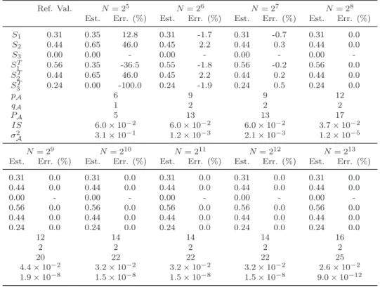
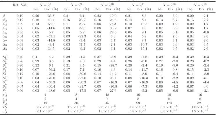
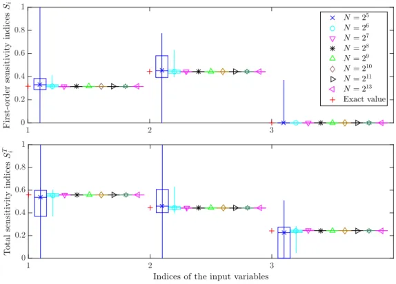
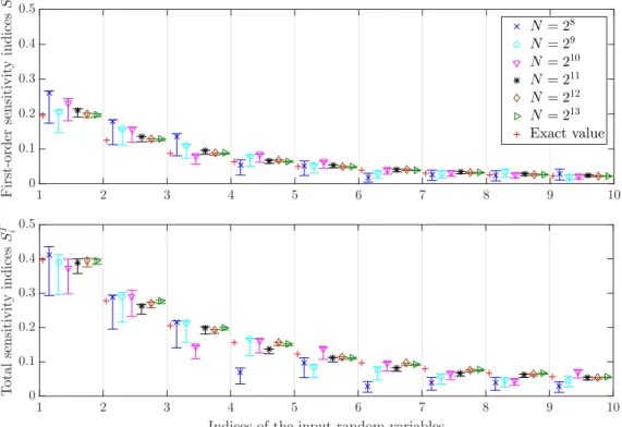
The PSI and the TSI are predicted quite well by the AFVB-PCE model using less number of significant terms in the polynomial basis as compared to the L-PCE model.. The PSI

Polynomial Chaos Expansion for Global Sensitivity Analysis applied to a model of radionuclide migration in randomly heterogeneous

Such assessment is possible using global sensitivity analysis, an approach able to analyze the variance of the output and determine the individual effects of each parameter

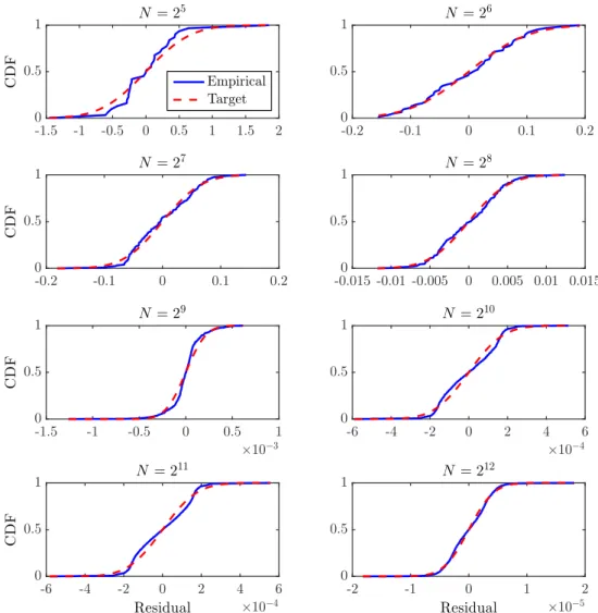
Generally, CDF can be estimated in three ways: (a) analytical calculation (b) standard MC sim- ulation (c) meta-model MC simulation –i.e., genera- tion of an experimental design of

Un large panel de gènes codant pour des protéines, de potentiels lincARN nouvellement prédits, mais aussi un nombre important d’éléments inter- géniques tels que des

RESUME : Cet article propose une histoire « quantitative » de la pensée économique en France à travers l’histoire de la structure doctrinale du corps des Professeurs

In the following, the adaptive weight behavior of the adaptive algorithm (15), called non-negative LMS, is studied in the mean and mean-square senses for a time-invariant step size

This magnetic field is associated with the electric current originating from the connecting wires (connected to the current generator at the ground surface), the injection current on