HAL Id: tel-01146310
https://hal.archives-ouvertes.fr/tel-01146310
Submitted on 29 Apr 2015
HAL is a multi-disciplinary open access archive for the deposit and dissemination of sci-entific research documents, whether they are pub-lished or not. The documents may come from teaching and research institutions in France or abroad, or from public or private research centers.
L’archive ouverte pluridisciplinaire HAL, est destinée au dépôt et à la diffusion de documents scientifiques de niveau recherche, publiés ou non, émanant des établissements d’enseignement et de recherche français ou étrangers, des laboratoires publics ou privés.
size and mobility of electronic bubbles and positive ions
in all phases of helium
Frédéric Aitken
To cite this version:
Frédéric Aitken. New thermodynamic model to predict the formation, size and mobility of electronic bubbles and positive ions in all phases of helium. Electric power. Université de Grenoble, 2014. �tel-01146310�
G2Elab - Laboratoire de Génie Électrique de Grenoble
Site : Polygone scientifique
HABILITATION A DIRIGER DES RECHERCHES
présentée par
Frédéric AITKEN
(Chargé de recherche au CNRS) Le 9 décembre 2014
RAPPORTEURS :
Thierry Belmonte Institut Jean Lamour, Nancy Armando Francesco Borghesani University of Padova, Italy Henry Glyde University of Delaware, USA
EXAMINATEURS :
Christophe Baudet LEGI, Grenoble
James Roudet G2ELab, Grenoble
CONTENU
I INNTTRROODDUUCCTTIIOONNGGEENNEERRAALLEE... ii T THHEEMMAATTIIQQUUEEEETTAAXXEESSDDEERREECCHHEERRCCHHEE... 3 A A TTHHEERRMMOODDYYNNAAMMIICC MMOODDEELL TTOO PPRREEDDIICCTT TTHHEE FFOORRMMAATTIIOONN, , SSIIZZEESS AANNDD MMOOBBIILLIITTIIEESS OOFF E ELLEECCTTRROONNCCAAVVIITTIIEESSAANNDDPPOOSSIITTIIVVEELLYYCCHHAARRGGEEDD’S’SNNOOWWBBAALLLLSS’’ IINNAALLLLFFLLUUIIDDPPHHAASSEESSOOFF H HEELLIIUUMM... 11 P PRROOJJEETTSSDDEERREECCHHEERRCCHHEE... 59Le document est divisé en deux grandes parties : la première relate globalement l’ensemble de mes axes et thématiques de recherche effectués jusqu’à aujourd’hui tandis que la deuxième est consacrée à la description d’un certain nombre de perspectives et projets futurs de recherche.
Dans le détail, la première partie est elle-même décomposée sous la forme de deux chapitres. Le premier chapitre exprime succintement un bilan de mes activités de recherche avec les principaux résultats obtenus tandis que le deuxième chapitre (en anglais cette fois-ci) consiste en une présentation détaillée des résultats majeurs obtenus sur un sujet très précis concernant la modélisation des mobilités ioniques et électroniques dans toutes les phases de l’hélium. Le choix de ce sujet provient du fait qu’il concerne la majorité de nos collaborations internationales et par conséquent il s’agit d’une activité de recherche forte du moment qui a conduit à des résultats sans précédent dans ce domaine.
P
P
R
R
E
E
M
M
I
I
E
E
R
R
E
E
P
P
A
A
R
R
T
T
I
I
E
E
T
T
H
H
E
E
M
M
A
A
T
T
I
I
Q
Q
U
U
E
E
E
E
T
T
A
A
X
X
E
E
S
S
D
D
E
E
R
R
E
E
C
C
H
H
E
E
R
R
C
C
H
H
E
E
I. Etude des micro-décharges électriques dans les liquides isolants ... 4 II. Electrocoalescence... 7 III. Réalisation d’un calorimètre pour mesurer les pertes des composants de l’électronique de puissance ... 8
Mon activité de recherche s’articule essentiellement autour du thème
« étude des micro-décharges électriques dans les liquides isolants ». C’est
une thématique très transversale qui va de l’étude des plasmas denses à l’étude de la mobilité des charges en passant par les phénomènes d’émission d’ondes de choc et de changement de phase hors de l’équilibre. Les compétences acquises dans ce sujet m’ont été utiles pour développer deux autres axes de recherche :
l’électrocoalescence et les mesures par calorimétrie des pertes des composants de l’électronique de puissance.
L’ensemble de mes activités de recherche est réalisé en collaboration étroite avec les autres chercheurs de l’équipe MDE : N. Bonifaci, A. Denat, P. Atten, F. Volino, O. Gallot-Lavallé et J-N. Foulc. Ainsi l’ensemble des stages et des thèses auxquels j’ai participé relève toujours de co-encadrements.
Les deux premières actions font l’objet de collaborations internationnales intenses et durables avec l’Institut des Hautes Températures (Moscou, Russie), l’Université de Leicester (Angleterre) et le SINTEF (Trondheim, Norvège).
Dans ce qui suit nous ne décrirons que les principaux résultats significatifs obtenus.
I. Etude des micro-décharges électriques dans les
liquides isolants
Une des activités de recherche historique de l’équipe MDE est l’étude de la conduction électrique dans les liquides isolants en géométrie pointe/plan et, plus précisément, la transition « isolant-conducteur » qui se produit au-delà d’une tension seuil, fonction de divers paramètres. Ce phénomène qui se produit à un champ électrique élevé (plusieurs MV/cm) est la conséquence d’avalanches électroniques dans un volume micronique lorsque la pointe est en polarité négative. Nous avons pu montrer que ces avalanches conduisent à la formation d’un plasma froid puis à l’émission d’une onde de choc dans le liquide et enfin à la formation d’une cavité (bulle) de taille micronique dont la dynamique dépend des caractéristiques du liquide et de la décharge. Cependant, la complexité de ces phénomènes loins de l’équilibre thermodynamique rend la détermination des paramètres de la décharge pratiquement impossible.
Afin de mieux comprendre les phénomènes de changement de phase hors-équilibre consécutif à une décharge localisée et leurs conséquences, les travaux de thèse de R. Qotba (2005) ont permis de démontrer très clairement d’une part que le fort amortissement des rebonds de la bulle ne provient pas de la compressibilité du liquide, ni des effets visqueux, ni des échanges thermiques à l’interface −et par conséquent il est normal qu’aucun des modèles actuels de dynamique ne puisse rendre compte de cet amortissement− et d’autre part que la
bulle arrivée à son rayon maximum passe par un équilibre instable tel que les conditions dans la bulle sont proches de la courbe de pression de vapeur saturante si la pression hydrostatiques P∞ est inférieure à la pression critique Pc
du fluide et proche de la ligne de Frenkel (i.e. courbe correspondante aux pics du
Cp dans la phase supercritique) si P∞ > Pc ; on démontre ainsi expérimentalement
qu’il existe un équivalent de « la chaleur latente de vaporisation » au-delà de la pression critique dont l’évolution en fonction de la pression et de la température n’a cependant rien à voir avec l’évolution de la chaleur latente de vaporisation. Plus précisément, l’énergie perdue par la bulle entre deux rebonds est principalement constituée de l’énergie emportée par l’onde de pression émise à la fin de chaque implosion, mais cette onde n’est pas générée dans le liquide comme le prévoient tous les modèles mais à l’intérieur même de la bulle.
Les études ci-dessus ont permis également de mettre en lumière la nécessité de bien maîtriser les équations d’état relatives à la phase liquide mais aussi à la phase mixte particulière de la cavité. Les phénomènes hydrodynamiques consécutifs à une décharge tels que les ondes de choc et les ondes de pression induites par la dynamique d’une bulle sont des sondes macroscopiques importantes qui rendent compte de la compressibilité du milieu. Ces travaux sur la compressibilité des fluides permettent d’avoir une meilleure compréhension des équations d’état couramment admises pour les fluides mais pas nécessairement justifiées ; en effet, les phénomènes hydrodynamiques auxquels nous sommes confrontés, sont de type « explosif » (temps de l’ordre de quelques nanosecondes), par conséquent pour pouvoir les modéliser il est nécessaire de connaître les équations d’état du fluide dans toute la gamme des conditions thermodynamiques rencontrées. Nous avons commencé par travailler sur l’argon car on dispose pour ce fluide de beaucoup de données précises ; c’est de plus un liquide atomique simple qui sert de référence pour la prédiction des propriétés thermodynamiques et qui sert également de calibration pour de nombreux instruments de mesure en thermodynamique. Aujourd’hui, l’équation d’état qui représente avec la meilleure précision possible les données expérimentales, du point triple à 700 K et de 0 MPa à 1000 MPa, est à base de polynômes (i.e. développement de type viriel) et d’exponentielles étirées sur la densité. Les coefficients, au nombre de 41, et les exposants (de l’ordre d’une grosse centaine) sont déterminés par des algorithmes de moindres carrés extrêmement sophistiqués, demandant une énorme puissance de calcul. Nous avons réussi à déterminer une équation d’état de l’énergie libre relativement simple qui couvre (avec la même résolution les données du NIST, de L’Air Liquide et de Ronchi), du point triple à 2300 K et à plus de 10 000 MPa à l’aide de seulement 26 coefficients (et environs 40 exposants), ce qui constitue une avancée significative. Contrairement au modèle en vigueur aujourd’hui, aucun terme polynomial n’est utilisé ce qui rend notre modèle extrapolable sans mauvaise surprise, robuste et stable vis-à-vis des approximations que l’on peut faire sur les valeurs numériques des coefficients et exposants. Nous pouvons de plus décrire les états
mécaniquement instables dans la région de coexistence liquide-vapeur, ce qui n’est absolument pas possible avec un modèle à base de polynômes. Notre modèle permet également une approche beacoup plus physique de la capacité calorifique à volume constant CV ; par exemple nous ne trouvons jamais de valeurs négatives
ni de divergences asymptotiques. Nous prévoyons de tester également notre modèle sur d’autres liquides, en particulier sur l’eau. Nos premières analyses montrent que notre approche sur l’argon peut être étendue à l’eau moyennant un terme de plus qui représente une ligne de base dans la modélisation du CV.
Les études précédentes sur les équations d’état et en particulier celles modélisant la compressibilité des liquides ont eu une application directe quant à la modélisation des mobilités des électrons et des ions positifs dans les différentes phases de l’hélium fluide. En effet, les seuls modèles existant à ce jour ne permettent nullement d’expliquer l’ensemble des données expérimentales dans n’importe quelle phase du fluide (que ce soit pour les ions positifs ou les électrons). Nous avons alors développé un modèle semi-empirique fondé sur la notion de volume libre (i.e. introduction d’une équation d’état traduisant la compressibilité d’un milieu fluide comprenant une certaine concentration de charges) qui permet de bien retrouver les mobilités observées expérimentalement dans une grande gamme de pression hydrostatique (0,1 à 10 MPa) et pour les différentes températures étudiées (entre 0,3 K et 300 K). Ces travaux ont été exposés pour partie dans la thèse de Z. Li (2008). Ces derniers sont maintenant exposés plus en détail dans le chapitre suivant.
Un autre outil remarquable de diagnostic des micro-décharges est l’étude spectroscopique car elle peut permettre d’obtenir un grand nombre d’informations comme la densité ou la température du milieu émissif, mais, l’augmentation de la densité du fluide introduit de nombreuses difficultés, aussi bien pour l’acquisition du spectre (les processus non radiatifs augmentent avec la fréquence des collisions) que pour son interprétation. En effet les théories susceptibles d’être utilisées à ces fortes densités nécessitent une analyse critique poussée afin de déterminer leurs domaines de validité en fonction de la densité du milieu et de la nature de la transition. La première difficulté de l’étude de l’élargissement des raies provient du fait qu’il y a un couplage entre le problème statistique dû aux chocs simultanés de différents perturbateurs et le problème de mécanique quantique dû à l’interaction entre un atome et un perturbateur. On sait résoudre le problème lorsqu’il est possible de séparer la moyenne sur le temps de la moyenne sur les coordonnées spatiales. Une première approximation consiste à supposer les perturbateurs fixes, dans ce cas la moyenne sur le temps disparait. Il ne reste qu’à moyenner sur les positions des perturbateurs dont l’influence est représentée par le potentiel d’interaction. Cette approximation est valable lorsque la durée d’une collision est beaucoup plus grande que la durée de vie des trains d’onde, c’est donc une approximation valable aux fortes densités. C’est aussi une approximation valable dans les ailes de la raie où la durée de vie des trains d’onde n’est plus limitée par les chocs mais par le temps intervenant
dans la fonction d’autocorrélation des trains d’onde. L’approximation inverse, dénommée « approximation d’impact », consiste à écrire que la durée d’un choc est très inférieure à l’intervalle entre 2 chocs ; c’est une approximation valable aux faibles densités et au centre de la raie.
Dans nos décharges, on se trouve souvent à la frontière entre l’approximation d’impact et quasi-statique. Afin de décrire complètement le profil de la raie sur tout son intervalle de longueur d’onde, nous devons souvent appliquer la théorie d’impact au centre de la raie, et la théorie quasi-statique sur les ailes. Afin de prendre en compte simultanément les deux profils adoptés pour décrire les différentes parties de la raie, nous devons effectuer une convolution d’un profil Lorentzien (PLor) et d’un profil déduit de l’approximation quasi-statique (PQS), c’est-à-dire :
(
) ( )
∫
−∞∞ Δ −= P λ ζ P ζ dζ
PT Lor QS .
L’obtention du profil de raie déduit de l’approximation quasi-statique (PQS) est un problème numériquement difficile et très délicat à résoudre du fait en particulier de la très forte oscillation des fonctions à intégrer et de leurs dynamiques rapides dans le temps lorsque le potentiel d’interaction évolue. L’approximation quasi-statique a fait l’objet de deux stages de Master qui nous ont permis d’identifier les difficultés et des premiers résultats encourageants ont été obtenus.
II. Electrocoalescence
L’électrocoalescence, c’est-à-dire la fusion de deux gouttes sous l’effet du champ électrique, est un problème relativement ancien mais qui a été très peu étudié depuis les articles publiés par G. Taylor dans les années 1965. C’est pourtant un problème qui concerne de multiples applications notamment pour éviter le stockage du pétrole sur les plates-formes pétrolières. En collaboration avec le SINTEF (institut de recherche norvégien), c’est un axe de recherche récent que nous développons au laboratoire. Le problème de la fusion de deux gouttes sous champ électrique est un problème d’instabilité très complexe, car ce mécanisme dépend de la taille des deux gouttes en présence, de l’intensité et de la fréquence du champ électrique, de l’écoulement hydrodynamique du liquide dans lequel les gouttes sont immergées, de la présence ou non de surfactants, etc. Afin d’étudier ce problème, nous avons commencé par envisager un problème plus simple où une goutte est remplacée par une sphère dure conductrice ou isolante et l’autre goutte par une interface plane eau/huile ou eau/air. Ce sujet a fait l’objet d’une toute première étude expérimentale en 2003 par un étudiant de
master, mais pour interpréter ces résultats nous devions admettre une valeur de tension interfaciale bien plus faible que la valeur théorique. Nous avons alors décidé de refaire toutes des expériences en couplant ces mesures à une mesure préalable de tension superficielle. Des mesures parfaitement correctes et cohérentes ont été enfin obtenues avec une interface eau-air. Malheureusement, nous sommes pour l’instant confrontés à d’énormes difficultés pour ce qui concerne une interface eau-huile : le problème des vibrations est ici particulièrement amplifié et les problèmes de pollution de l’interface modifiant la tension interfaciale se produisent systématiquement.
Toujours dans le cadre du contrat qui nous lie avec l’institut norvégien SINTEF, nous nous sommes attaqués au problème déjà plus réaliste de la déformation de deux gouttes initialement proches et soumises à une différence de potentiel. Un modèle avec sa résolution numérique a pu être obtenu lorsque les deux gouttes sont ancrées. En effet, dans le cas contraire où elles ne sont pas ancrées, il faut tenir compte, lors du rapprochement des interfaces, du film liquide qui se trouve chassé. Mais ce mouvement est très compliqué à modéliser car il affecte non seulement l’écoulement à l’intérieur des gouttes mais aussi la répartition de pression hydrostatique extérieure tout autour des gouttes. Seule une solution numérique avec des éléments finis ou des éléments aux frontières peut être envisagée. Ce problème ne relève pas d’un problème de déformation statique contrairement au cas des gouttes ancrées. Ainsi dans le cas des gouttes ancrées, un critère de stabilité statique a été obtenu et il est utilisé pour la calibration de simulations numériques plus complexes.
III. Réalisation d’un calorimètre pour mesurer les
pertes des composants de l’électronique de puissance
Suite à une interrogation formulée par l’équipe Electronique de Puissance (EP) du G2ELab, Olivier Gallot-Lavallé et moi-même avons décidé de nous lancer dans l’étude d’un calorimètre performant qui permettrait de mesurer la dissipation de chaleur de n’importe quel composant électrique. En effet, un calorimètre isotherme destiné à mesurer les pertes de condensateurs de puissance a été réalisé il y a une bonne quinzaine d’années au laboratoire lors de la thèse de B. Seguin (1997). Malheureusement ce calorimètre (fondé sur la prépondérance d’un transfert thermique par conduction entre le composant et la cellule de mesure) n’est pas adapté à des formes très variées des composants ; de plus la puissance qui est mesurée ne représente que partiellement la puissance dissipée par le composant (i.e. la puissance perdue par rayonnement est omise, ce qui rend la mesure de plus en plus imprécise au-delà de 300 K ; le flux rayonné dépasse à ce stade de 40% le flux transmis par conduction, ce dernier étant le
seul flux mesuré).
Compte tenu des nombreuses imperfections que nous avons relevées sur l’ancien calorimètre, les travaux de thèse de E. Obame N’Dong (2010) ont permis de réaliser un tout nouveau calorimètre de conception totalement différente du précédent : la conception est celle d’un corps noir régulé en température (i.e. cellule isotherme), à l’intérieur duquel le composant actif se trouve suspendu. L’ensemble est mis sous vide dans une enceinte réfléchissante et isolée.
Le dispositif unique que nous avons conçu et réalisé permet de s’affranchir de la forme géométrique du composant et il permet de faire des mesures dans une gamme de température allant de 200 à 400 K. Le composant électrique peut être alimenté par une tension arbitraire inférieure à 3 kV. L’analyse des résultats obtenus sur des composants dont les pertes sont connues a montré que l’incertitude de mesure était inférieure à 5% pour une gamme de puissance dissipée allant du mW au Watt. Ceci en fait un dispositif unique de par le monde et par conséquent un brevet a été déposé avec le CNRS.
Ce dispositif est actuellement utilisé par une startup issue de l’équipe EP (Electronique de Puissance) du laboratoire pour tester des composants de puissance très variés.
A
A
T
T
H
H
E
E
R
R
M
M
O
O
D
D
Y
Y
N
N
A
A
M
M
I
I
C
C
M
M
O
O
D
D
E
E
L
L
T
T
O
O
P
P
R
R
E
E
D
D
I
I
C
C
T
T
T
T
H
H
E
E
F
F
O
O
R
R
M
M
A
A
T
T
I
I
O
O
N
N
,
,
S
S
I
I
Z
Z
E
E
S
S
A
A
N
N
D
D
M
M
O
O
B
B
I
I
L
L
I
I
T
T
I
I
E
E
S
S
O
O
F
F
E
E
L
L
E
E
C
C
T
T
R
R
O
O
N
N
C
C
A
A
V
V
I
I
T
T
I
I
E
E
S
S
A
A
N
N
D
D
P
P
O
O
S
S
I
I
T
T
I
I
V
V
E
E
L
L
Y
Y
C
C
H
H
A
A
R
R
G
G
E
E
D
D
’
’
S
S
N
N
O
O
W
W
B
B
A
A
L
L
L
L
S
S
’
’
I
I
N
N
A
A
L
L
L
L
F
F
L
L
U
U
I
I
D
D
P
P
H
H
A
A
S
S
E
E
S
S
O
O
F
F
H
H
E
E
L
L
I
I
U
U
M
M
1. Introduction ... 17 2. Method ... 242.1. The free volume model for normal and superfluid phases... 24
2.2. The free volume model for gaseous and supercritical phases ... 29
2.3. Derivation of vapour pressure curves for van der Waals systems and the implications for electrons and ions in helium... 31
3. Discussion ... 35
3.1. The role of viscosity... 35
3.2. Electrons... 38
3.3. Positive ions ... 44
3.4. Interpretation of mobility in the superfluid phase... 50
3.5. Interpretation of the maxima in the pressure dependence of the hydrodynamic radius ... 50
4. Conclusion... 52
5. References ... 53
6. Appendix ... 54
6.1. Equations of state for normal and superfluid phases ... 54
LIST OF FIGURES
Figure 1: Pressure dependence of electrons mobility in gaseous helium on the isotherm 4.19 K. The experimental data has been taken from Levine et al. (1967)... 18 Figure 2: Pressure dependence of electrons mobility on the isotherm 1.76 K in the superfluid phase. The experimental data has been taken from Brody (1975). The red curve is the best calculated pressure dependence of mobility from eq. (5) associated to the bubble model eq. (9) with no surface tension. The
theoretical variation with pressure is always opposite to the experimental data. ... 20 Figure 3: Pressure dependence of our hydrodynamic radius and momentum cross-section in supercritical helium at 11 K calculated using state of the art models and the thermodynamic description presented here (see text). . 21 Figure 4: Pressure dependence of our hydrodynamic radius and momentum cross-section in
supercritical helium at 3.9 K calculated using state of the art models and the thermodynamic description presented here... 21 Figure 5: Experimentally derived mobilities of positive ions in liquid helium at 2.63 K [Keshishev et al., 1969], 3 K and 4 K [Meyer et al., 1962]. The dashed dotted lines show mobilities calculated using the Atkins model for the respective experimental conditions. For each temperature two calculations were performed using σ = 0 N/m and σ = 0.1 N/m as surface tension coefficient. The
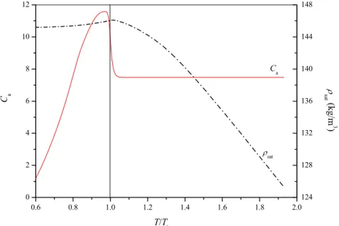
calculated mobilities deviate at low and high pressures irrespective of the chosen surface tension coefficient. The variation with pressure deviates consistently from the experimental data... 23 Figure 6: Evolution of the size-proportionality parameter Ca with temperature for electrons. Ca is
constant in the normal liquid phase but increases sharply when the superfluid phase transition is reached. This increase is correlated to the known maximum of the saturated vapour pressure density of helium, ρsat, in the region of the phase transition. The increase of helium density means
that more space is available for electrons and thus explains why Ca shows a maximum... 26
Figure 7: Pressure dependence of different kinds of calculated radius for an electron cavity in the superfluid phase on the isotherm 1.602 K... 29 Figure 8: Saturated vapour pressure of positive ions in helium and of pure helium. The vapour pressure curve of pure helium is a fit to data from NIST... 34 Figure 9: Pressure dependence of positive ions mobility in the supercritical phase along the isotherm 6.35 K.
Data were recorded from our experimental set-up. The two curves are calculated from our model using eq. (22) to (25)... 35 Figure 10: Calculated mobility for positive ions on the van der Waals saturated vapour pressure curve eq. (39) from 2.4 K to 23 K... 35 Figure 11: Viscosity of normal helium from NIST data for a number of isobars... 36 Figure 12: Experimental data of normal viscosities along the isotherm 1.83 K from the saturated vapour pressure curve to the melting line. The blue diamonds in normal liquid helium are calculated from the
extrapolation of formula given by NIST... 37 Figure 13: superposition of the effective viscosity surface (with orange mesh) on the normal viscosity surface (with black mesh) from the saturated vapour pressure curve to the solidification line and from the isotherm Tλ,max
to the isotherm 0.8 K. The black vertical surface represents the λ-line states... 38 Figure 14: Mobility and hydrodynamic radius in the low temperature region of normal liquid helium at 2.2 K and 3.0 K. The experimental data has been taken from Meyer et al. (1962). ... 39 Figure 15: Mobility and hydrodynamic radius in the high temperature region of normal liquid helium at 4.2 K and 4.5 K. The experimental data has been taken from papers published by Meyer et al. (1962) and by Keshishev et al. [1969] and by ourselves. ... 39 Figure 16: Electron mobility and hydrodynamic radius in the supercritical region of helium. The experimental data shown has been taken from Harrison et al. (1973), Jahnke et al. (1975),
Borghesani et al. (2002) and ourselves... 40 Figure 17: Electron mobility and hydrodynamic radius in supercritical region of helium between 45 and 80 K. The experimental data shown has been taken from Jahnke et al. (1975) and Borghesani et al. (2002)... 41 Figure 18: Electron mobility and hydrodynamic radius in gaseous helium at low temperatures of helium between 3.65 and 4.19 K. The experimental data shown has been taken from Levine et al. (1967)... 42 Figure 19: Electron mobility and effective radius in superfluid helium. Experimental data
reproduced from Brody (1975)... 43 Figure 20: Electron mobility. Experimental data reproduced from Ostermeier (1973)... 44 Figure 21: Mobility and hydrodynamic radius of He ions in the low temperature region of normal
liquid helium at 2.2 K, 2.63 K and 3.0 K. The experimental data has been taken from Meyer et al. (1962) and Keshishev et al. (1969)... 44 Figure 22: Mobility and hydrodynamic radius of He ions in the high temperature region of normal liquid helium at 4.2 K and 4.5 K. The experimental data at 4.2 K has been taken from Meyer et al. (1962) and Keshishev et al. (1969)... 45 Figure 23: Mobility and hydrodynamic radius of He ions in supercritical helium. Data were
recorded from our experimental set-up... 46 Figure 24: Mobility and hydrodynamic radius of He ions in supercritical helium at 135 K. Data were recorded from our experimental set-up. ... 47 Figure 25: Mobility and effective radius of He ions in superfluid helium for temperatures in the range from 1.4 to 1.8 K. Experimentally determined mobility is nicely matched by our theoretical values. The experimental data has been taken from Brody (1975)... 48 Figure 26: Modeled and experimentally determined positive ion mobility for the temperature range of 0.4 to 1 K. The experimental data has been taken from Ostermeier (1973)... 49 Figure 27: Modeled and experimentally determined positive ion mobility and hydrodynamic radius of positive ions in helium for temperatures in the region of the λ-line showing the effect of λ-line
crossing with increasing pressure. The experimental data has been taken from Goodstein et al. (1974) and Keshishev et al. (1969)... 50 Figure 28: Saturated vapour pressure curve of pure helium and Frenkel curve (open circles). The position of the maxima of the hydrodynamic radius of electron (stars) and ions (squares) in the P-T plan is shown as well. ... 52
Physical Constants for Helium
M Molar mass M = 4.002 6 g mol–1 Tc Critical temperature Tc = 5.195 3 K Pc Critical pressure Pc = 0.22637 MPa ρc Critical density ρc = 69.642 kg m-3Tλ,max λ-line maximum temperature
Tλ,max = 2.176 8 K
Pλ,max λ-line pressure corresponding to Tλ,max
Pλ,max = 0.004 856 5 MPa
Tλ,min λ-line minimum temperature
Tλ,min = 1.767 3 K
Pλ,min λ-line pressure corresponding to Tλ,min
1. I
NTRODUCTIONElectrons and positive ions are microscopic probes frequently used to explore transport, diffusion and quantum properties of liquid helium. Electrons introduced into liquid helium localise and build large cavities with radii up to 20 Å (at 4.2 K and 1 bar), depending on the pressure. The formation of such voids results from the repulsive interaction between ground state helium atoms and electrons because of the Pauli principle and the very long range van der Waals-like attraction. Positive ions in liquid helium behave the opposite way. Here, electrostrictive forces between the positive charge and the surrounding polarised helium atoms dominate and attract the helium atoms towards the positive centre. As a consequence a dense, solid-like shell of helium is built, which is why the term ’snowball’ or ’Atkins-snowball’ is often used [Atkins-1959].
Information of the size of the space that electrons and ions occupy in helium is difficult to obtain in a direct fashion. Infrared spectroscopy of electrons in liquid helium has been employed [Grimes et al.-1990]. The spectral features show a distinct pressure dependence and the bubble model has been employed to derive the change of size with pressure. Recent advances in density functional theory (DFT) has made it possible to calculate the sizes of electron cavities as a function of pressure up to temperatures of 3 K as well as the corresponding energies which match very well with the spectroscopic data [Grau et al.-2006].
Thanks to the charged nature of electrons and ions the measurement of their mobility is relatively straightforward to measure using electric fields. The mobility is related to a hydrodynamic radius via the well known Stokes law for spherical objects η ψπ μ r e = Stokes (1)
where ψ is a coefficient which depends on the boundary conditions at the interface. The deduction of the radius requires no other knowledge than the dynamic viscosity, η, of the fluid. A number of restrictions nevertheless apply. First, the hydrodynamic radius is generally not identical with the intrinsic radius of the moving object. For example, the object may drag a tightly bound solvation with it, which would cause the hydrodynamic radius appear larger. Second, the no-slip conditions requires sufficiently dense fluids. Decreasing densities are commonly accounted for using the more general Millikan-Cunningham equation
) (1 = Stokes
MC μ φ
μ + (2)
where μMC is the Millikan-Cunningham mobility and φ the Millikan-Cunningham factor.
In He gas at low density the electron is considered as free and its mobility
0
1/2 0 ) (2 3 4 = T k m Nq e b e π μ (3)
where e and m are the electron charge and mass, respectively, e N the number density, q the momentum transfer cross-section (constant for He, q =5⋅10−20m2)
and kB the Boltzmann constant. A modified version of eq. (3) to account for the simultaneous interaction with several atoms at increased density has been reported as well [Atrazhev-1984].
) (1
= μ0 πλeNq
μ − (4)
where μ refers to the corrected mobility and Nqλe to the ratio between the electron de Broglie wavelength λe and the classical mean free path length Nq1/ . Equation (4) takes only first order density corrections into account and is therefore only valid for moderate corrections μ/μ0 >0.3. But in any case eq. (4) cannot reproduce the experimental data much better than eq. (3). Figure 1 shows typical pressure dependence experimentally observed in gaseous helium and the corresponding gas kinetics law eq. (3) for electrons.
Figure 1: Pressure dependence of electrons mobility in gaseous helium on the isotherm 4.19 K. The
experimental data has been taken from Levine et al. (1967).
In the superfluid phase, for temperatures above 0.6-0.8 K, the classical approach is to admit that the mobility of the charge carriers is mainly due to the scattering mechanism with rotons. For lower temperatures, two other scattering mechanisms must be taken into account: phonon scattering and scattering by atoms of 3He. Then the accepted hypothesis is to assume that the different type of diffusers act independently of each others so that the total scattering rate τ−1 is
assuming that the mobility is described by the Langevin law μ =
(
e M)
τ , whereM is added mass of the carrier, then the mobility of a charge carrier is written
finally: 1 He 1 phonon 1 roton 1 3 − − − − = μ +μ +μ μ (5)
As usual, the calculation of the roton-limited mobility is deduced from the Boltzmann transport equation such that the roton drag force whatever the carrier is expressed by the following relationship:
(
)
k( )
( )
x T k T P e B G 9 4 , exp 4 2 0 roton σ ρ π μ ⎟⎟⎠= h ⎞ ⎜⎜ ⎝ ⎛ Δ (6) with( )
* 2 0 2 4M k x= β h ρ and G( )
x = 1/x+e−x[
x×K0( ) (
x − 1+x)
×K1( )
x]
where T kB 1 = β , σis here an effective cross-section, k0 ≈ 1.91 Å-1 is the wave number at the minimum of the dispersion curve in the roton’s region and Δ
(
P,T)
is the energy gap of rotons.The usual calculation of the phonon-limited mobility is obtained from the Boltzmann transport equation such that the phonon drag force whatever the carrier is expressed by the following relationship:
( )
∫
∞ ∂ ∂ − = 0 2 2 phonon 6 dk k k n k e mt kσ π μ h (7)where nk is the equilibrium phonon distribution function and σmt
( )
k is themomentum-transfer cross section which is defined in terms of the differential cross-section σ
( )
k,θ as( ) (
k =∫
−) ( )
k dΩmt θ σ θ
σ 1 cos , (8)
Now the differential cross-section is calculated from the scattering of classical sound waves from an elastic sphere: boundary limit conditions are different for positive ions and for electrons and also electrostrictive effects must be taken into account for the case of positive ions.
For the contributions of 3He impurities, the obvious model leads to hard-sphere scattering. By treating the impurities as a Maxwell-Boltzmann gas, the drag force relationship is a proportional function of T . The constant of propotionality is an empirical adjustable parameter.
Figure 2 shows the typical pressure dependence of electrons mobility along an isotherm for experimental data and calculated from the classical bubble model eq. (5) to (9). The best classical approach shows systematically a wrong description of the experimental data with an opposite curvature of pressure dependence of mobility along isotherms. The same opposite pressure variation is
also observed for positive ions mobility when using the same appraoch. 0,0 0,5 1,0 1,5 2,0 2,5 3,0 0,00 0,05 0,10 0,15 0,20 0,25 0,30 μ (cm 2 /V. s ) P (MPa) Data of Brody
Best classical approach
Figure 2: Pressure dependence of electrons mobility on the isotherm 1.76 K in the superfluid phase. The
experimental data has been taken from Brody (1975). The red curve is the best calculated pressure dependence of mobility from eq. (5) associated to the bubble model eq. (9) with no surface tension. The
theoretical variation with pressure is always opposite to the experimental data.
Finding a coherent description of ions and electrons mobility in different density regions, especially the crossover from gas kinetic to Stokes flow is a challenge. An implicit challenge is that ions and electrons in helium are expected to change their structure depending on the density. For sufficiently low densities, for example, the growth of Atkins snowballs will not happen. Likewise, under low pressure conditions where the helium density is very low the establishment of electron bubbles makes no sense.
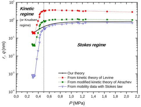
0,0 0,2 0,4 0,6 0,8 1,0 1,2 1,4 1,6 1,8 2,0 2,2 10-4 10-3 10-2 10-1 100 101 Kinetic regime (or Knudsen regime) Stokes regime r -, q (nm ) P (MPa) Our theory
From kinetic theory of Levine
From modified kinetic theory of Atrazhev From mobility data with Stokes law
Figure 3: Pressure dependence of our hydrodynamic radius and momentum cross-section in supercritical helium
at 11 K calculated using state of the art models and the thermodynamic description presented here (see text).
0,00 0,01 0,02 0,03 0,04 0,05 0,06 0,07 0,08 10-5 10-4 10-3 10-2 10-1 100 101 Stokes regime r -, q (n m) P (MPa) Our theory
From kinetic theory of Levine
From modified kinetic theory of Atrazhev From mobility data with Stokes law
Kinetic regime
(or Knudsen regime)
Figure 4: Pressure dependence of our hydrodynamic radius and momentum cross-section in
supercritical helium at 3.9 K calculated using state of the art models and the thermodynamic description presented here.
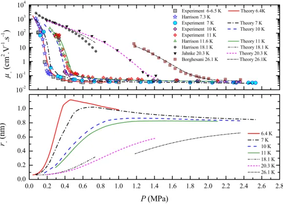
Figure 3 and Figure 4 illustrate this situation on the example of the pressure dependence of the hydrodynamic radius of electrons. In supercritical helium at 11 K above 0.5 MPa, electrons form cavities. Cavity radii derived from mobility measurements using Stokes law lie in an accepted size range. Instead, momentum cross-section produced using the kinetic or the amended kinetic
theory produce values that are unrealistically large. Helium at 3.9 K turns from a liquid-like behaviour into a gas behaviour when the pressure decreases lower than 0.06 MPa. The hydrodynamic radius derived from the Stokes equation, which appears correct in the liquid phase, falls to unrealistic low values below pressures of 0.06 MPa. In contrast, standard gas kinetic theories predict cross-sections close to the electron scattering lengths, which is correct, but they fail to predict realistic values for pressures where helium has become enough dense.
Being able to model mobilities over large density ranges and specifically being able to cover the crossover from the liquid to the gas phases would provide us insight into how electron cavities and ion snowballs grow. A special case is the superfluid phase of helium which is characterised by the presence of two components, the normal fluid and the superfluid component whose concentration depends on the temperature and the presence of foreign entities such as electrons or ions.
The present work addresses these questions. We develop thermodynamic state equations for electrons and He ions in helium and employ the free volume model to derive the thermodynamic radius. In general terms, the free volume model relates the size of foreign objects, i.e. solute molecules within a fluid to the size occupied by a free volume unit cell, (V-b)/N, using a simple power law between the two in first approximation. The state equations of P, V and T include parameters which are calibrated using experimentally determined mobilities reported in the literature. The mobilities, μ, are related to the size via the hydrodynamic radius, r , in the Stokes-Einstein equation and by introducing the Millikan-Cunningham factor specifically developed for electrons and ions in helium to account for a large density coverage of our thermodynamic approach, including the gas, supercritical, liquid and superfluid phases.
Electronic mobilites in helium have previously been modeled using the
bubble model. The bubble model has been very popular in the past because of its
simplicity. It expresses the total energy of the cavity created by the electron as a sum of inner energy, surface energy and volume energy
P r r r m h E e 3 2 2 2 cavity 3 4 4 8 = + π σ + π (9)
h is Planck’s constant, m the electron mass, e σ the surface tension coefficient1 and P the hydrostatic pressure. By minimising the radially dependent energy an equilibrium radius can be obtained. Electron mobilities calculated from radii predicted by the bubble model match experimental data only poorly and only in a very limited pressure and temperature range. The model essentially considers how an electron cavity is compressed when external hydrostatic pressure is applied. We will later see that such a compression is not the only effect and that
1 In the normal liquid phase, the state equation σ
( )
ρ commonly used is deduced from theMacleod-Sugden empirical correlation function. In the superfluid phase, σ is commonly scaled with the ratio
( )
( )
0 1 0 1 ρ ρ ρ ρ c cwhere c1 represents the first sound velocity and ρ0 the density at zero
regimes exist where cavity radii increase with increasing pressure. In this case the bubble model clearly fails. A further disadvantage is that the surface tension σ is only known along the vapour pressure curve. Since electron cavities can be established in much larger P,T ranges than the vapour pressure line, the bubble model will necessarily become increasingly inaccurate. In fact, the best accuracy is obtained for surface tension σ equal to zero which is not coherent.
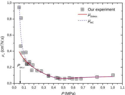
A similar approach has been taken to model mobilities of He ions in helium by Atkins (1959). In the first step the size of an ion cluster in helium is calculated. Atkins used a similar approach as for the electrons and modified eq. (9) by addition of an electrostriction energy term. Atkins assumed a priori a solid structure, with the consequence that all other parameters are from the solid phase. This requires good knowledge of the state equation in the liquid and at the melting line. Furthermore, Atkins assumed for the fluid a radial density decrease around the ion cluster caused by the electrostrictive forces. All other relevant quantities such as viscosity were derived from these densities and consequently showed the same radial dependence. A consequence of the radial dependence of the fluid properties is that the drag force is no longer governed by Stokes law and a numerical resolution of the Navier-Stokes equations has to be done for this particular problem. Apart from these specific conditions, the Aktins model suffers from the same deficiencies as the electron bubble model, as it can be seen on Figure 5. 0 1 2 3 4 5 6 7 1E-3 0.01 0.1 1 Meyer 3 K Atkins σ = 0 mN/m Atkins σ = 0.1 mN/m Meyer 4.2 K Atkins σ = 0 mN/m Atkins σ = 0.1 mN/m Keshishev 2.63K Atkins σ = 0 mN/m Atkins σ = 0.1 mN/m μ+ (c m 2 /V .s ) P (MPa)
Figure 5: Experimentally derived mobilities of positive ions in liquid helium at 2.63 K [Keshishev
et al., 1969], 3 K and 4 K [Meyer et al., 1962]. The dashed dotted lines show mobilities calculated
using the Atkins model for the respective experimental conditions. For each temperature two calculations were performed using σ = 0 N/m and σ = 0.1 N/m as surface tension coefficient. The calculated mobilities deviate at low and high pressures irrespective of the chosen surface tension
coefficient. The variation with pressure deviates consistently from the experimental data. In this work we present thermodynamic state equations for electrons and ions helium in all phases. We show that the free volume model combined with a specifically formulated Millikan-Cunningham factor is well suited to derive size
information. With this approach we are able to model the compression of electron cavities and positively charged snowballs in helium caused by increasing hydrostatic pressure. We are also able to observe the increase of the hydrodynamic radius with increasing pressure in low density regimes which we interpret as the growth of electron cavities and snowball clusters as well as the gradual establishment of a boundary layer. Our theoretical framework is equally well suited to model electron and ion mobilities in the superfluid phase of helium and derive size information. The phenomena in the superfluid phase match well with a two-phase model where the concentration of normal fluid helium depends on the temperature as well as on the presence of impurities. A certain critical density of normal fluid helium is needed to establish a boundary layer and Stokes flow conditions. In many ways the superfluid regime resembles the cross-over from flow in liquid helium to flow in gaseous helium.
To complement experimentally derived mobilities of electrons and ions in helium reported in the literature we have also conducted measurements of I(V) curves in micro-corona discharges in point-plane geometry [Li et al.-2008, Aitken
et al.-2011]. These measurements fill gaps in the existing literature specifically
for supercritical helium.
2. M
ETHOD2.1. The free volume model for normal and superfluid phases
The free volume model derives the size of unknown foreign microscopic objects that coexist in thermal equilibrium at low concentration [Doolittle-1951, Cohen et al.-1959, Miyamoto et al.-1973]. A key assumption is the proportionality of the volume occupied by an unknown foreign object and the volume
(
V −b)
/Noccupied by a single free volume unit cell. Here, V designates the total volume of a set of N helium atoms. This proportionality means that the volume of the foreign object changes in the same fashion as the volume, V , of the helium, in other words the compressibilities are proportional. Strictly, the covolume, b, of all hard-core helium atoms in the cell has to be replaced by a different covolume
b′ because the foreign particles contribute to the covolume with a different hard-core volume. The free volume V is equal to the difference f V −b′ for which an state equation is formulated. We write for the free volume V = f V −b′ and for the volume of a charged foreign object V : a
N V const
Va = f (10)
where const is the proportionality constant.
For small concentrations of foreign particles the total volume of the system will not change much and we can relate the volume occupied by the impurities to
Π + P T Nk V B f = (11)
Here kB is the Boltzmann constant, and Π is the internal pressure that accounts
for all attractive interactions, i.e. between the impurities and the pure helium atoms.
If we assume a spherical shape of the ’unit cell’ occupied by the charged foreign objects of volume V = a (4/3)π(r−a)3 we can express the effective cavity
radius, r−a, by: 3 4 3 = Π + − P T k C a r B a π (12)
a is the non-compressible radius and represents the ’radius’ of the free foreign object, consequently r−a represents the cavity radius in excess of the ‘hard-core’ length. For convenience, we write Ca instead of 31/const where the index a is
related to properties of a charged foreign particle a, i.e. a will change if another impurity with different interaction is considered. Ca is a measure of how volume-changes of a mixed phase relate to the pure phase. Therefore Ca represents the ratio of the compressibilities of the mixed and the pure fluid. Equation (12) is at the heart of this work since it relates size to a thermodynamic state equation.
Finding the cavity radius r reduces to the problem of determining C and a
Π , which is achieved by calibration of the parameters of the state equations to the hydrodynamic radius derived from experimentally determined mobility and by developing an expression for the internal pressure Π in eq. (12) that shows consistent variation of the mobility with P , T and ρ. Generally, one expects different terms for Π depending on the thermodynamic phase and the type of impurity because the compressibility changes significantly. Sufficiently far from the melting line and from the critical isotherm, the expression of Π is predominantly characterised by a van der Waals like behaviour such that the general form is:
• for ions: 2 ion =αρ
Π
• for electrons:
{
2 correction term}
2 0 ⎟ + ⎠ ⎞ ⎜ ⎝ ⎛ = Π − αρ T T e
where α is a universal constant such that [Aitken et al.-2011]:
2 3 m kg / bar 0.00796 = ⎟⎟ ⎠ ⎞ ⎜⎜ ⎝ ⎛
α . In both expressions, it appears the term αρ2 which
expresses the simple van der Waals-type behaviour. The correction term which appears for electrons models the density-dependence in a more sophisticated way to better include the long-range interaction beyond a Lennard-Jones C -type 6
contribution. Very close to the melting line, an another correction must be applied on both expressions of Π due to the “feeling” of this phase transition. The detailed expressions for Π are given in Appendix.
We note that the values of Ca along isotherms are calibrated by using the
experimental data of mobilities along the saturated vapour pressure curve. As an example, the temperature dependence of Ca for the electrons and the correlation
with the temperature dependence of the density is shown in Figure 6. We can observed that Ca is independent of temperature in most of the normal liquid
phase but when approaching the λ -line from the liquid phase Ca increases
rapidly, passes through a maximum at Tλ,max and decreases until it reaches zero at a given temperature T (Ca ≅ 1.2 K for electrons). A zero value of Ca corresponds to a size of the electrons equal to the scattering length, a. Such a behaviour is not unexpected and can be understood in terms of gas phase-like flow of electrons in the superfluid phase. The increase of Ca at Tλ,max indicates that the size of
electron cavities expands. Although we are unable to comment on the microscopic origin of this expansion, an increase of the electron cavity size correlates well with the temperature dependence of density in pure helium: at Tλ,max the density increases distinctively. This means that for the electrons more space is available, the cavities grow and Ca consequently increases. The same kind of dependence
with temperature is observed for ions except that Ca is not as constant in the
normal liquid phase as for electrons. This means that the compressibilities between positive ions and pure liquid helium differs from the corresponding ratio for electrons. It can be understood in terms of the stronger binding between the core of the ionic cluster and the solvation shell. The detailed expresions for Ca are
also given in Appendix.
0.6 0.8 1.0 1.2 1.4 1.6 1.8 2.0 0 2 4 6 8 10 12 124 128 132 136 140 144 148 Ca T/Tλmax ρsat ρ sa t ( kg/ m 3 ) Ca
Figure 6: Evolution of the size-proportionality parameter Ca with temperature for electrons. Ca is
constant in the normal liquid phase but increases sharply when the superfluid phase transition is reached. This increase is correlated to the known maximum of the saturated vapour pressure density of helium, ρsat, in the region of the phase transition. The increase of helium density means
that more space is available for electrons and thus explains why Ca shows a maximum.
After C and the parameters in a Π have been determined eq. (12) can be used for calculation of radii, r . Since the dynamic viscosity of helium is well documented for a wide pressure range and temperatures above the upper
superfluid phase transition temperature, Tλ,max, it is possible to calculate mobility
via the Stokes-Einstein eq. (1) which assumes different forms for electrons and ions: η π μ − − r e e = 4 (13) η π μ + r e 6 = ion (14)
The factor of 4 or 6 depends on the boundary conditions at the interface [Batchelor-1970], i.e. a hollow object such as an electron cavity is described using eq. (13). We note that the radius calculated in eq. (12) should be interpreted as a
hydrodynamic radius since the reference for this calculation is mobility data and
validity of Stokes flow. The hydrodynamic radius reflects boundary layer effects, where the boundary layer can assume widths of similar size than an electron cavity radius. In addition, the intrinsic radius of electron cavities and of Atkins-snowballs is not defined.
To account for boundary layer effects in low-density regions where Knudsen numbers Kn≥1 (i.e. the concept of continuous medium is no more valid), the Stokes-Einstein eq. (1) has to be modified by the Millikan-Cunningham factor, φ, such that μMC = μStokes(1+φ). Knudsen regime is observed in the superfluid phase for temperatures below T . We will see that by using an Ca
appropriate formulation of the Millikan-Cunningham factor, it is possible to model the strong increase of mobilities in the superfluid phase below 1 K. The general form of the Cunningham factor φ for the superfluid phase can be written as:
( )
exp correction term50 3 2 1 sat for superfluid + ⎥ ⎥ ⎦ ⎤ ⎢ ⎢ ⎣ ⎡ ⎟⎟ ⎠ ⎞ ⎜⎜ ⎝ ⎛ − − ⎟ ⎟ ⎠ ⎞ ⎜ ⎜ ⎝ ⎛ = Λ Λ Λ ≤ c c c c a T T T T T T x a C ρ ρ ρ ρ ρ ξ φ (15) with ⎥ ⎥ ⎦ ⎤ ⎢ ⎢ ⎣ ⎡ ⎟ ⎟ ⎠ ⎞ ⎜ ⎜ ⎝ ⎛ − ⎟ ⎟ ⎠ ⎞ ⎜ ⎜ ⎝ ⎛ ⎟ ⎟ ⎠ ⎞ ⎜ ⎜ ⎝ ⎛ − = = sat exp exp ρ ρ ρ ρ n T T n C C a C a a T T T x (16),
where T represents the temperature for which CCa a = 0 and ρn the density of the
normal liquid part in the superfluid phase. The function x(T) given by eq. (16) is an analogon2 to the Knudsen number: for temperatures less than
a
C
T , x increases
and represents in increasing gas-phase-like behaviours of the superfluid phase. The value of the exponent Λ must be considered as equal to one but if we want 3
2 It is important to note that the natural definition of x would be to use the ratio ρ ρ
n not only on the saturated vapour pressure curve but for all P and T in the superfluid phase. However, due to the uncertainty on the values of this ratio, we restricted its use only on the saturated vapour pressure curve. The consequence of this choice leads to a relationship more complicated that it should be on the expression of ξ (x).
to satisfy with high precision all the data coming from different authors a small deviation from one can be introduced. The function ξa
( )
x is determined by a calibration of mobilities along the saturated vapour pressure curve. The correction term leads to the displacement towards high pressures of mobility’s maximum along isotherms as it is experimentally observed. Detailed expressions are given in Appendix.The superfluid phase is here understood in terms of the classical two-fluid concept where the superfluid component has per definition viscosity zero and only the normal fluid component contributes to viscous flow. Hence in the superfluid phase a distinction must be made between the effective radius r eff
deduced from eq. (12) and the hydrodynamic radius rhydro. Both of them are related by the following relation:
eff hydro = r r n ρ ρ (17)
It appears that the density of the normal liquid part, ρn, is therefore a key parameter in our theoretical framework. The relation between density, ρ, normal liquid density, ρn, and superfluid density ρs is as follows
ρ ρ ρ ρn s − 1 = (18)
For the ratio ρn/ρ we have in the following employed the values valid on the saturated vapour line reported by Donelly et al. We note that below 1.2 K these values differ considerably from values reported by NIST, who propose the following equation to generate ρn/ρ as a function of both T and P .
⎪⎩ ⎪ ⎨ ⎧ ⎟ ⎠ ⎞ ⎜ ⎝ ⎛ − − + + otherwise , 0.55 1 0.02863 1 0.45 < < 0 if ) ( ln = ) , ( 6 3 3 2 2 1 x x x C x C x x C P T s ρ ρ (19) where , ) ( 1 = P T T x λ − (20) ) (P
Tλ is not directly available in the literature as a function of P. Therefore, Tλ(P) is obtained upon inversion of the following relationship reported by Arp [1990]. atm) (in = ) ( 6 5 4 4 3 3 2 2 1 0 y b e b y b y b y b y b b T Pλ + + + + + (21) with y =T −Tλ,max.
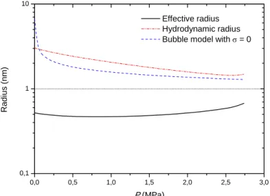
0,0 0,5 1,0 1,5 2,0 2,5 3,0 0,1 1 10 Radi us (n m) P (MPa) Effective radius Hydrodynamic radius Bubble model with σ = 0
Figure 7: Pressure dependence of different kinds of calculated radius for an electron cavity in the superfluid
phase on the isotherm 1.602 K.
As an example of the distinction between different kinds of radius, Figure 7 shows the different electron cavity radius at 1.602 K: for this isotherm we find that reff ≈0.55nmand rhydro ≈2.5nm. We can observe that the hydrodynamic radius values are very close to the calculated values using the bubble model eq. (9) with no surface tension (i.e. without surface tension the bubble model gives its greatest radius values). But unfortunately, the bubble model eq. (5) to (9) is not able to reproduce the pressure variations of mobilities along any isotherm in the superfluid phase contrary to our approach. It is useful to note that in our approach only the normal liquid component participates in the formation of cavities and their compression. We will see that this concept represents experimental observation very well.
2.2. The free volume model for gaseous and supercritical phases
In the gaseous and supercritical phases, the relation between the volume of a charged foreign object V and the free volume a V is a little more complex f
than the proportionnality given by eq. (10) because in these phases “condensation” and compression of the cavities can be both observed. Then a general form for the variations of the radius impurity with density and temperature is now:
(
)
(
)
(
)
⎥ ⎥ ⎦ ⎤ ⎢ ⎢ ⎣ ⎡ − + − 2 1 1 / ) ( exp / 1 / = 0 0 0 ε ε ε κ γ f a f f V V T V V V V a a r (22)in which V0/Vf can be replaced simply by:
T P V V f Π + δ = 0 (23)
where ε1 ,ε2 ,γ and δ are constants which depend on the kind of impurity and they are determined once from one isotherm of experimental mobilities data. The coefficient γ reflects more or less the amplitude of the pressure range corresponding to the condensation regime: larger is this coefficient and narrower is the pressure range.
The internal pressure Π which appears in eq. (23) is identical to the expression for the normal liquid phase for ions and for electrons the expression is similar to those for the normal liquid phase but now ρsat is replaced by ρc; the two expressions are then linked together at the critical point by using the crossover function: ⎟ ⎟ ⎠ ⎞ ⎜ ⎜ ⎝ ⎛ ⎟ ⎠ ⎞ ⎜ ⎝ ⎛ × − Θ 20 crit exp = ) ( T T T θ c (24)
Equation (22) exhibits now two kinds of behaviour along an isotherm: at low pressure the radius growth with the increase of pressure (i.e. condensation regime) until it reaches a maximum and then it decreases (i.e. compression regime). The pressure corresponding to the maximum increase when the temperature of the isotherm is increased and this phenomenom is mainly driven by the function κa(T) which is essentially a simple exponential decay of temperature.
In the gaseous and supercritical phases, the density can now vary from almost zero value to high values such that Knudsen number Kn can vary from zero value to many orders of magnitude hence the Millikan-Cunningham equation μMC = μStokes(1+φ) must be systematically used. The general form of the Cunningham factor φ is slightly different for the gaseous and the supercritical phase such that:
( )
⎪ ⎪ ⎪ ⎩ ⎪⎪ ⎪ ⎨ ⎧ ⎟⎟ ⎠ ⎞ ⎜⎜ ⎝ ⎛ ⎟⎟ ⎠ ⎞ ⎜⎜ ⎝ ⎛ = ⎥ ⎥ ⎦ ⎤ ⎢ ⎢ ⎣ ⎡ ⎟⎟ ⎠ ⎞ ⎜⎜ ⎝ ⎛ − ⎥ ⎥ ⎦ ⎤ ⎢ ⎢ ⎣ ⎡ ⎟ ⎠ ⎞ ⎜ ⎝ ⎛ − = Γ Γ Γ Γ gas c supercriti 0 gas 3 2 2 1 exp exp φ ρ ρ φ ρ ρ χ ρ ρ φ φ c c c c a c T T T T Kn T (25)The value of Γ2 is 0 or 1 depending of the kind of impurity. The value of Γ 3 must be considered as equal to zero but if we want to take into account with high precision all the data coming from different authors with different experimental set-up a small variation of Γ with the temperature can be introduced. The 3 function χa(T) is essentially a simple power law of temperature but again if we want to satisfy the various data from different authors with different experimental set-up some small deviation terms must be introduced which lead to a more sophisticated dependance with temperature.
We note that the form of eq. (25) is similar to the first term of the Millikan-Cunningham factor in the superfluid phase given in eq. (15). This shows
similarities of the flow behaviour, which can be understood within the framework of the two-fluid model. The effective density in the superfluid phase is given by the normal fluid density which decreases with temperature, hence the variation of this effective density is similar as the variation of density in the supercritical phase.
2.3. Derivation of vapour pressure curves for van der Waals systems and the
implications for electrons and ions in helium
By introducing reduced variables for ρ, P and T it is possible for van der Waals-type interacting particles to establish a state equation in dimensionless form and to establish a vapour pressure curve, Pσ (T), in dimensionless form. If the critical parameters are known it is then possible to calculate the vapour pressure curve. We will briefly review the procedure and calculate the critical parameters for electrons in supercritical helium. The same concept will later be applied for positive ions in helium.
c P P P =~ (26) c ρ ρ ρ~= (27) , = ~ c T T T (28)
Here the pressure, density and temperature have been reduced with respect to the critical pressure, P , critical density, c ρc, and critical temperature,
c
T . For any point on the saturated vapour pressure curve, the pressure of the gas
phase is the same as the pressure of the liquid and likewise for the temperature, however the densities of the gas and liquid phase are different.
L L L v v v P P T ρ ρ ρ ρ ρ ρ σ σ σ ~ 8 ~ 3 ) ~ 3 ~ ( = ~ 8 ~ 3 ) ~ 3 ~ ( = ~ + 2 − + 2 − (29)
We rearrange eq. (29), replace the temperature, T~σ , and the pressure, P~σ, respectively, and obtain the following two equations:
8 ) ~ ~ )( ~ )(3 ~ (3 = ~ v L L v Tσ −ρ −ρ ρ +ρ (30) ) ~ ~ (3 ~ ~ = ~ L v L v Pσ ρ ρ −ρ −ρ (31)
The coexistence curve P~σ(T~σ) is then obtained in a parametric form.
On the coexistence curve the chemical potentials of the liquid and gas phases are equal per definition and we can write:
![Figure 5: Experimentally derived mobilities of positive ions in liquid helium at 2.63 K [Keshishev et al., 1969], 3 K and 4 K [Meyer et al., 1962]](https://thumb-eu.123doks.com/thumbv2/123doknet/15048318.693818/28.892.213.678.595.935/figure-experimentally-derived-mobilities-positive-liquid-helium-keshishev.webp)