Design of Plate-Fin Tube Dehumidifiers for Humidification-Dehumidification Desalination Systems

Design of Plate-Fin Tube Dehumidifiers for

Humidification-Dehumidification Desalination Systems

The MIT Faculty has made this article openly available. Please share

how this access benefits you. Your story matters.

Citation Sievers, Martin, and John H. Lienhard V. “Design of Plate-Fin Tube Dehumidifiers for Humidification-Dehumidification Desalination Systems.” Heat Transfer Engineering (April 23, 2014): pp. 1-76.

As Published http://dx.doi.org/10.1080/01457632.2014.916153

Publisher Taylor & Francis

Version Author's final manuscript

Citable link http://hdl.handle.net/1721.1/88095

Terms of Use Creative Commons Attribution-Noncommercial-Share Alike

Design of Plate-Fin Tube Dehumidifiers for

Humidification-Dehumidification Desalination Systems

Martin Sievers1,2 and John H. Lienhard V1,∗

1

Department of Mechanical Engineering, Massachusetts Institute of Technology, Cambridge, MA 02139-4307, USA

2

Present Address: MAHLE Behr GmbH & Co. KG, Siemensstraße 164, 70469, Stuttgart, Germany

ABSTRACT

A two-dimensional numerical model of a plate-fin tube heat exchanger for use as a dehumidifier in a humidification-dehumidification (HDH) desalination systems is developed, because typical heating, ventilating, and air conditioning (HVAC) dehumidifier models and plate-fin tube dehumidifier geometries are not intended for the considerably higher temperature and humidity ratio differences which drive heat and mass transfer in HDH desalination applications. The experimentally validated model is used to investigate the influence of various heat exchanger design parameters. Potential improvements on common plate-fin tube dehumidifier designs are identified by examining various methods of optimizing tube diameter, and longitudinal and transverse tube spacing to achieve maximum heat flow for a given quantity of fin material at a typical HDH operating point. Thicker fins are recommended than for HVAC geometries, as the thermal conductive resistance of HVAC fins restricts dehumidifier performance under HDH operating conditions.

∗

INTRODUCTION

The ever-increasing demand for clean water is in part satisfied by desalinating seawater or brackish water with the humidification-dehumidification (HDH) process [1, 2]. The development of HDH desalination systems has made remarkable progress in recent years [3-11]. However, most improvements have concentrated on new system configurations, thermodynamic analysis, and proof-of-concept experiments. Solar heaters [12, 13], humidifiers [14] and thermal compressors [15] are the HDH desalination system components so far investigated in most detail. Dehumidifiers, however, have often been adopted from existing heating, ventilating, and air conditioning (HVAC) technology, for which they are mass produced at low price, rather than developed in the HDH context. An intensive study on flat-plate and plate-fin tube dehumidifiers for HDH desalination systems has been performed [16, 17] one step towards improved HDH desalination system configurations. Thiel and Lienhard [18] investigate in-tube condensation for dehumidification in an HDH desalination system and provide a literature survey on condensation of water vapor from an air-steam mixture. The current paper investigates plate-fin tube heat exchangers as components for integration into HDH desalination system design.

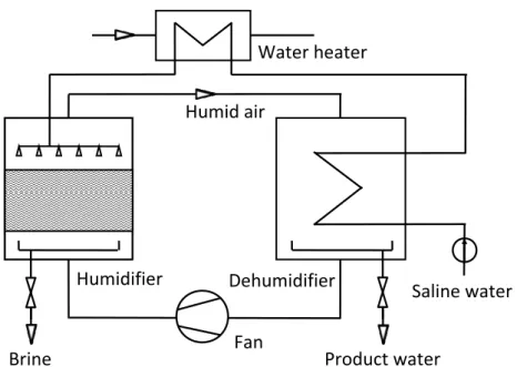
Narayan et al. [3] describe in detail various HDH desalination systems and designs. Figure 1 shows a simple closed-air open-water water-heated HDH desalination system. The main components are a humidifier, a dehumidifier, and a water heater. In the humidifier, warm saline water is partially evaporated into an air stream. Nearly saturated air exiting from the top of the humidifier is transported to the saline water-cooled dehumidifier. Within the dehumidifier, the air humidity decreases with decreasing temperature, and some of the water vapor condenses producing pure water which is collected at the bottom of the dehumidifier. This product water can be used for the intended purpose. Latent and sensible heat are transferred from the air to the saline water side to preheat the saline water. In a closed-air system, dehumidified air is recirculated to the humidifier. In a water-heated cycle, the preheated saline water is further heated by a (solar) water heater before being sprayed into the humidifier. Saline water not vaporized in the humidifier is discarded. Many variants of this basic architecture exist [3, 4].

Heat Exchangers for Dehumidification

Various heat exchanger types have been used as dehumidifiers in HDH desalination systems. The majority of reviewed papers [3] refer to plate-fin tube heat exchangers (cf. Figure 2, top), the most economical type for HVAC dehumidification. This type is often adopted for HDH processes as well. Air flows around the tubes and along the plate-fins in direction of gravity; saline water passes through the tubes. Saline water may be distributed from a port manifold to all tubes, or the tubes may be set up in a multi-pass configuration. In process industry and HVAC systems, a z-configuration and adjustment of the flow cross-section achieves equal mass-flow rates in all tubes. In a multi-pass heat exchanger, return bends route the saline water through several tubes. The result is a single-pass or multi-pass crossflow configuration.

Plate fins enhance air-side heat transfer by increasing the air-side surface area. They can be flat, or corrugated or perforated to induce turbulence. Common standardized geometries for air-cooling and dehumidifying heat exchangers are according to [19]: outside tube diameters 8.0, 10.0, 12.5, 16.0, 20.0, and 25.0 mm; longitudinal and transverse tube spacing ranging from 15 to 75 mm; fin spacing from 1.4 to 6.4 mm; and according to [20] fin thickness from 0.005 to 0.008 inches (0.127 to 0.203 mm). In refrigeration applications outside tube diameters not larger than 10 mm are common nowadays. To prevent excessive fouling and erosion seawater velocities between 1.5 m/s and 2.4 m/s are recommended [21, 22].

Criteria for the selection of heat exchanger materials are cost, mass, corrosion resistance, thermal conductivity and possible machining. Plate-fin tube heat exchangers in HVAC systems typically consist of Cu tubes with Al fins [19], permitting high thermal conductivity at moderate cost. Circular tubes are expanded to press-fit the surrounding plates.

In a corrosive atmosphere, however, this standard Cu-Al combination forms an electrochemical cell which induces corrosion. CuNi alloys, which have a higher corrosion resistance, are standard for the tubes of marine plate-fin tube heat exchangers. For seawater-operated HDH dehumidifiers the SOLDES project [23] recommends CuNi 90/10 for the tubes, Al or Cu for the fins, and stainless steel 304L for the frames, casing

and collecting basin. In practice, Houcine et al. [24] reported corrosion of these dehumidifier materials after only six months of operation.

Improved corrosion resistance is achieved by adding a small proportion of Fe to the tube alloy. On the basis of over 20 years’ experience at a seawater corrosion test facility at Helgoland, North Sea, Germany, Happ [21] recommends CuNiFe 90/10 tubes with Cu fins. To slow down or even inhibit corrosion of the fins and extend the life time of the dehumidifier a coating layer on the air side is useful. The carry-over of saline water droplets from the humidifier to the dehumidifier needs to be avoided by the system design.

DEHUMIDIFIER MODEL

A numerical model is developed for detailed analysis of the dehumidifier, and the resulting equations are presented here. The segment-by-segment (or cell method) [25] is applied. In contrast to standard two-zone models [19, 26, 27], the heat exchanger is not only subdivided into one dry and one wet section, but is discretized into several segments in the air flow and saline water flow directions to achieve a two-dimensional solution instead of an average outlet state for this 2 or 3 dimensional problem. The air and saline water outlet states are determined for given air and saline water inlet conditions and heat exchanger geometry.

The model incorporates the following assumptions and features:

• Steady-state conditions apply to heat and mass transfer

• Mass transfer is determined by the Chilton-Colburn heat and mass transfer

analogy [28]

• The Lewis number Le = 0.865 [29] is used, which applies accurately to HDH

operating conditions [16], instead of the common assumption Le = 1.0

• The high-rate mass transfer model with a logarithmic mass transfer driving force is applied [28]

• The surface area of a segment is either fully dry or fully wet

• The effect of condensation-induced fluid motion normal to the main air flow direction is taken into account by the Ackermann correction factor [30]

• The thermal conductive resistance of the condensate film which forms on the heat exchanger surface is taken into account by Nusselt’s condensation theory [28]

• The energy balance includes the enthalpy change of the condensate in air flow

direction

• The velocity reduction in each segment due to condensation is taken into

account

• As the heat transfer coefficient, air temperature and humidity ratio do not change much within each segment, heat conduction in the tube and fins is assumed one dimensional in the radial direction in a segment, but different from segment to segment

• The heat exchanger is adiabatic with respect to the environment (no heat

losses)

• Heat and mass transfer are calculated at constant pressure.

Governing Equations for the Wet Control Volume

Figure 2 (center) illustrates the two-dimensional discretization of the plate-fin tube heat exchanger in the y and z directions. Figure 2 (bottom) shows an enlarged view of the wet control volume with the variables used.

Heat and mass transfer are simulated at constant pressure and are not coupled to the pressure drop calculation, as the pressure drop has minor influence on the fluid properties and the heat transfer calculation. The pressure drop is calculated after the heat and mass transfer calculation is completed and takes the temperature and velocity distribution into account.

The derivation of governing equations for the plate-fin tube heat exchanger model is analogous to Sievers and Lienhard [17]. The equations comprise the water mass balance

a da pw m d m

d& =−& ω , (1)

the air-side energy balance

(

pw pw

)

da a pw pw pw pw a

dadh d m h m dh m dh h dm

m Q

d& = & + & = & + & + &

− , (2)

sw swdh m Q

d& = & , (3)

the mass transfer equation

) ( 622 . 0 1 622 . 0 1 ln 1 f t s I a m a w pa ta pw Le d A A M M c h m d + + + = − _η ω ω & , (4)

and the heat transfer between the air and the condensate film

(

)

( ) 622 . 0 1 622 . 0 1 ln 1 f t s I a m a w pa wg I a ta a da Le d A A M M c h t t h dh m +             + + + − = − _η ω ω ζ & , (5)

with the Ackermann correction factor [30]

( )

1 exp−Φ − Φ − = ς where ta pa f t s pw h c A A d m d ) ( + = Φ η & (6)

to include the influence of condensation-induced fluid motion towards the interface. The temperature of the interfacial boundary between product water and air is

(

)

(

)

) ( 622 . 0 1 622 . 0 1 ln 2 ) / ln( ) ( 1 1 2 1 2 2 f t s tpw pw pw I a m a w pa wg I a tpw ta tsw t f t s sw I A A d h h m d Le M M c h t t h h h d d k d d d A A d Q d t t + −             + + + − +       + + + = − η ω ω ς η & & , (7)

and the mean product water temperature according to Sadasivan and Lienhard [31] is

(

)

        −       + + +         − + = −         − + = I tsw t f t s sw pw I I pw I pw t h d d k d d d A A d Q d t Pr t t t t t 1 2 1 2 2 0 2 ) / ln( ) ( 228 . 0 683 . 0 Pr 228 . 0 683 . 0 η & . (8)

The exponent m of the Lewis number in the heat mass transfer anology in Eqs. (4), (5),

and (7) equals the Prandtl number exponent m of the heat transfer equations. Typically m

= 1/3 is used for the heat mass transfer analogy [28].

This system of equations is used to determine the distribution of the heat flow transferred to the saline water side Q& , the mass flow of product water m&pw, the humidity

ratio ωa, the air temperature t , the product water temperature a tpw, the saline water

temperature tsw, and the temperature of the interfacial boundary t . The humidity ratio at I

the interfacial boundary is taken to be ω_I =ω_sat(p,t_I).

The thermophysical properties of dry air are derived from the composition of dry air [32]. Molar masses from Coplen [33], the specific gas constant of dry air Rda = Rm/Mda =

0.287117 J/(mol K), and the ratio of the molar masses of water and dry air Mw/Mda =

0.62217 ≈ 0.622 are used. The thermophysical properties for humid air are calculated from HuAir [34], those for water from IAPWS-IF97 [35, 36], and those for standard seawater of salinity 35 g/kg from Sharqawy et al. [37] as saline water.

The governing equations for the dry or wet control volume are solved for each segment in sequence from the air inlet to the air outlet; beginning with an initial estimate of the saline water outlet temperature. The wet section begins once the air-side surface temperature is lower than the air dew point temperature. Subsequent segments in the air downstream direction are also assumed to be wet. The system of governing equations for dry or wet control volumes is solved by a trust region dogleg algorithm [38].

Heat Transfer Equations for Plate-Fin Tube Heat Exchangers

Air-side heat transfer in a plate-fin tube heat exchanger depends upon its geometry, i.e. tube diameter, tube spacing, number of tube rows, fin spacing, fin thickness, and

surface geometry, and is quantified either by the Colburn j-factor

3 / 2 3 / 2 3 / 1 ) / ( w c Pr h Pr c A m h Pr Re Nu j pa c a ta pa c a ta ρ = = = & (9)

or by the Nusselt number Nu

a h ta k d h Nu = . (10)

Available equations only cover a limited set of geometries. The four air-side heat transfer equations for staggered tube arrangement [39-42] listed in Table 1 are applied here. (The tubes are staggered in air-flow direction and in-line transverse (normal) to air-flow

direction as shown in Figs. 2, 6, and 7.) For these equations, the air flow velocity )

/( _{c a}

a

c m A

w = & ρ is derived from the minimum free flow area Ac,min between the tubes

and the fins (Ac = Ac,min). Various characteristic lengths x are used to calculate the

Reynolds number Rex. Wang et al. [42] use the fin collar diameter dc = d2+2 df when the

tubes are surrounded by a collar of fin material. McQuiston [39] has derived j-factor equations for dry surfaces and for wet surfaces with film or dropwise condensation, whereas Gray and Webb [40], Pacheco-Vega et al. [41], and Wang et al. [42] have determined j-factor equations for dry surface only. Gray and Webb’s j-factor equation [40] is also published in [43].

Apart from these equations derived specifically for plate-fin tube heat exchangers of a particular geometry, Gnielinski’s parallel-plate duct heat transfer equations [44, 45], listed in Table 1, may be applied to air-side heat transfer over a wide range of heat

exchanger geometries. Here the Reynolds number Redh = ρ w dh/µ is calculated from the

air flow velocity

ψ ψ ρ 1 1 m 0 a s d -s w s d -s L W w f f a = = & (11)

with the air face velocity w0, where s is the fin spacing, df the fin thickness and

l tX X d22 4 1 π

ψ = − the air-side porosity of the plate-fin tube heat exchanger. The hydraulic

diameter is dh = 4 Vs/As = 4 Vs/(At + Af ), where As is the wetted surface area enclosing

the wetted volume Vs.

Local heat transfer coefficients in circular tubes [46, 47] are applied on the saline water side. Heat transfer through the condensate film is described by Nusselt’s condensation theory [28]. For all equations, thermophysical properties are evaluated at the arithmetic mean fluid temperature between inlet and outlet of each segment; the temperature dependence of the fluid properties between bulk and wall or interface surface temperature within a segment is neglected, i.e. (Pr/PrI)0.11 = 1.

Fin and Surface Efficiency for Plate-Fin Tube Heat Exchangers

To simplify the simulation, heat conduction through the tubes and fins is modeled using fin and surface efficiencies. The fin efficiency is

e temperatur surface tube at fin by d transferre flow heat fin by d transferre flow heat actual = f η . (12)

and the surface efficiency is [48]

f tf t tt f f tf t tt s A h A h A h A h + + = = η η e temperatur surface tube at tube and fin by d transferre flow heat tube and fin by d transferre flow heat actual . (13) where At is the air-side heat transfer surface area of the tube not occupied by fins, Af is the

air-side heat transfer surface area of the fins and At+Af is the total air-side heat transfer

area. The surface efficiency is used in the air-side heat transfer calculation in Eqs. (4), (5), (7), and (8). When equal heat transfer coefficients htt on the tube surface and htf on

the fin surface are assumed, the surface efficiency is simply ) 1 ( 1 f f t f s A A A η η − + − = . (14)

The fin efficiency for thin fins of constant thickness df << Xt, df << Xl is [49]

2 / ) 2 / tanh( 2 2 d m d m f Φ Φ = η , (15)

where m is the fin parameter and Φ d2/2 the weighted fin height. This equation is based

on the analytical solution for a fin of uniform cross section, corrected to allow for different fin geometries.

For dry heat transfer, the fin parameter is

2 / 1 0 2         = = f f ta d k h m m . (16)

For calculation purposes, the plate fin is subdivided into hexagonal fins around each tube as shown in Fig. 7. For these, the calculation parameter

      +       − = Φ 2 2 ln 35 . 0 1 1 d d d de e ₍₁₇₎

with the equivalent fin diameter de

2 / 1 3 . 0 27 . 1 _      − = R c R e b X b d , (18) where

2 / 1 2 2 ) 4 / 1 ( l t c X X X = + (19)

for staggered tubes is used. Xl is the longitudinal tube spacing in the air-flow direction, Xt

the transverse tube spacing normal to the air-flow direction, and bR is the smaller of the

two distances 2 Xl and Xt:

t l l R t l t R X X X orb X X X b = for2 ≥ =2 for2 < (20)

In-line configurations, whose heat flow is poorer, are rarely used in plate-fin tube heat exchangers and are thus not considered here. The better heat transfer characteristics of staggered tubes are more suited to heat-transfer equipment, despite the higher pressure drop.

For combined heat and mass transfer (wet heat transfer) the fin efficiency is lower than in the equivalent dry case. A solution using the Chilton-Colburn heat and mass transfer analogy is adapted from [50] to represent the situation:

) 1 ( 2 2 0 2 B b m m = + , (21) 3 / 2 Le c h B pa fg = , (22) I tip fin I sat tip fin sat t t t t b − − = ( ) ( ) 2 ω ω . (23)

The fin tips are represented by the edge of the hexagons of Fig. 7. There are no partially wet fins in the system investigated, as the relative humidity of the moist air entering the dehumidifier in HDH desalination systems is high. The fin tip temperature is determined by solving ) 2 / cosh( 1 ) 1 /( ) 1 /( 2 2 0 2 0 Φ = + + − + + − d m B b C B t t B b C B t t I a tip fin a , (24) a a a b t C0 =ω − 2 − 2 , (25) I I tip fin I sat tip fin sat I sat t t t t t t a − − − = ( ) ( ) ( ) 2 ω ω ω . (26)

A high fin efficiency, i.e. a fin temperature close to the tube temperature, requires direct mechanical contact between fin and tube around the entire tube perimeter. Corrosion, thermal expansion and the manufacturing process can lead to a significant contact resistance. Contact is perfect and permanent only if the fin is integral to the tube.

Pressure Drop Determination

Air and water experience a pressure drop when they pass through the heat exchanger. A trade-off between good heat transfer characteristics with a small heat transfer area (low investment costs) against a low pressure drop with low energy consumption by fans and pumps (low operating costs) is normally required.

In general the pressure drop in the heat exchanger is

(

)

∑

∑

∆ + ∆ +∆ +∆ = ∆ i i f i dec i g j j M p p p p p _{, , , ,} , (27)

where ∆pM,j is the pressure drop associated with inlet and outlet on the air side or return

bends on the saline water side; ∆pg,i is the geodetic pressure drop, ∆pdec,i is the

deceleration pressure gain; and ∆pf,i is the frictional pressure drop per tube row i.

Using a total pressure loss coefficient K, the pressure drops at inlet, outlet and in the return bends are calculated from

2 2 w K p_M = ρ ∆ (28)

where K = 4 for each return bend [51] in the saline water flow, and Kays’ data [52] for K = f(Re,geometry) for inlet contraction and outlet expansion for air flow. The pressure

drop ∆pg resulting from the geodetic height change is low and therefore neglected.

The air-side humidity ratio change results in a significant deceleration pressure rise

a pw a c dec A m p ω ρ ρ ∆       −       = ∆ 1 1 2 & . (29)

On the saline water side the pressure change due to velocity variation is negligible. The frictional pressure drop in the saline water flow is expressed as

2 2 sw sw h f w d z p =ξ∆ ρ ∆ (30)

where ξ is the (Darcy-Weissbach) friction factor. Smooth tubes are assumed, so the friction factor is independent of the surface roughness. For tube flow the Hagen-Poiseuille and the Konakov friction factors are applied:

dh Re

64 =

(

)

(

)

2 10 15 log 8 1 − − = . Re_dh . ξ for 2300 < Redh < 106. (32)

The air-side frictional pressure drop is determined as a combination of the drag of the flow across the tube ∆pft and the drag of the flow along the fins ∆pff as proposed by Gray

and Webb [40] ft ff f p p p =∆ +∆ ∆ . (33)

This approach separates the two effects that cause a pressure drop and thus provides a physical basis for an extrapolation to new geometries. Two different equations are used to determine ∆pff for the fins and ∆pft for the tube in Eq. (33). The pressure drop for the fins

(plates) is calculated either according to Gray and Webb [40]

2 2 , c a c f GW f ff w A A p =ξ ∆ ρ ∆ , (34) where 318 . 1 2 521 . 0 2 ,GW 0.508Red (Xt /d ) f − = ξ (35)

with the air flow velocity at the minimum free flow area w_c = m&_a/(ρ_a A_c,min) in Eq. (34)

and in Red2, or according to Hagen-Poiseuille and Konakov [53]

2 2 , w d y p _a h HK f ff ξ ρ ∆ = ∆ (36) dh HK f Re 96 , =

ξ for laminar flow Redh < 2300 (37)

(

)

(

)

2 10 2/3 1.5 log 8 . 1 − − = Redh ξ for 2300 < Redh < 106 (38)

with w according to Eq. (11) and Redh as mentioned there. The pressure drop associated

with the tube

2 2 c a t ft w p =ξ ρ ∆ (39)

is either taken from Žukauskas [54] or determined from the following equations from Gaddis and Gnielinski [55]

            + − − + = 1000 200 Re exp 1 Re Re 2 25 . 0 2 2 d d tt d tl t ξ ξ ξ (40)

(

)

(

)

[

]

(

)(

)

(

)(

)

1.6 2 2 2 2 5 . 0 2 / / / 4 75 . 0 6 . 0 / 280 d X d X d X d X t l t l tl π π ξ − + − = for Xl/d2 ≥0.5 2Xt/d2+1 (41)

(

)

(

)

[

]

(

)(

)

(

)(

)

1.6 2 2 2 2 5 . 0 2 / / / 4 75 . 0 6 . 0 / 280 d X d X d X d X c l t l tl π π ξ − + − = for Xl/d2 <0.5 2Xt/d2+1 (42)

(

)

3 3 08 . 1 2 1 01 . 0 1 4 . 0 85 . 0 / 2 . 1 5 . 2 _      − −       − + − + = l t t l t tl X X X X d X ξ , (43)

where Red2 is calculated with the air-flow velocity wc at the minimum free flow area and

Xc from Eq. (19).

The equation of Gray and Webb [40] is restricted to the range given in Table 1 within which it is more accurate than Eqs. (31) and (32); otherwise the alternative is applied.

No suitable method of determining the wet pressure drop in the condensate-air flow on the air side could be found. The correction by Wang et al. [56], though accurate, is limited in range, which is problematic when varying the geometry.

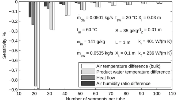
Sensitivity Analysis

The sensitivity analysis shown in Fig. 3 reveals the effect of an increasing number of segments on the simulation result. The number of segments used to discretize a single heat exchanger tube is varied from 10 to 100 in increments of 10. Only the changes in: air temperature difference from inlet to outlet, product water temperature difference from inlet to outlet, heat flow to the saline water and the air humidity ratio difference from inlet to outlet are shown here. The product water temperature difference is determined as the difference between air inlet temperature and product water outlet temperature. The salinity is that of standard seawater. Here and in all the following calculations, standard seawater is used as an example for saline water. For saline water with different salinity, similar results are found.

A comparison of sensitivity and validation results implies that 20 segments per tube suffice for significant accuracy within short simulation time. So all simulations are done with 20 elements per tube for optimized performance. For 20 segments per tube the grid convergence index (GCI) [57] is -2.15 % for the air temperature difference from inlet to

outlet, -2.09 % for the product water temperature difference, -0.54 % for the heat flow, and -0.35 % for the humidity ratio difference between inlet and outlet.

Validation

Data from McQuiston’s experiments for plate-fin tube dehumidifiers [58], Series 10000 with condensation of water from humid air, are used to validate the numerical model. The heat exchanger’s geometrical data are: four staggered copper tubes in air flow

direction with d2 = 9.957 mm spaced longitudinally at Xl = 16.764 mm and transversely

Xt = 25.400 mm, and df = 0.1524 mm thick plain aluminum fins with collars spaced at s

= 3.175 mm.

On the seawater side, the equations for heat transfer in tubes are applied. To compensate for condensation-induced fluid motion, the Ackermann correction [Eq. (6)] is always applied to the air-side heat transfer coefficient. For the low mass transfer HVAC experiments considered, it has a negligible influence on the results. The experimental and simulated results are compared in Fig. 4, and the maximum and root mean square (rms) deviations are listed in Table 2. Apart from the air temperature difference between inlet and outlet ∆ta, the highest accuracy is achieved by Gray and Webb’s equation. That

equation should therefore be applied if the heat exchanger geometry lies within its validity range (cf. Table 1).

The heat transfer equations for parallel-plate duct flow (Gnielinksi [44, 45]) lead to less accurate results compared to the j-factor equations specifically fitted for the plate-fin tube geometry. But their validity range is wider than that of the j-factor equations by McQuiston [39], Gray and Webb [40], Pacheco-Vega et al. [41], and Wang et al. [42]. Equations for parallel-plate duct flow thus apply to a broad range of geometries, as is necessary when optimizing the heat exchanger geometry.

Since McQuiston’s j-factor equation is accurate to no better than about 10% for Series 10000, the model with this equation operates within the achievable accuracy.

Unexpectedly, a dry j-factor equation with a suction correction achieves the best agreement with the experimental results.

A validation of the different pressure drop equations for tube and fins is shown in Fig. 5. No combination is adequate. Combinations of Gray and Webb’s equation for the fins

with Žukauskas’ results (rms 44%) or with Gaddis’ equation (rms 37%) for the tube agree poorly. Gnielinski’s combination of the Hagen-Poiseuille and Konakov parallel-plate flow equation with Žukauskas’ results for the tube leads to larger deviations of rms 57%. However, the wide range of applicability of this combination is advantageous. The use of Wang et al.’s [56] wet pressure drop correction, valid only for a limited range of geometries, reduces the rms to an acceptable 16%.

Inside its validity range, the Gray and Webb heat transfer and pressure drop equation is combined with Žukauskas’ result. Outside of this range, the parallel-plate duct heat transfer equation and the parallel-plate duct pressure drop equation are applied.

Comparison with other Models

Several different dehumidifier models are available in the literature, e.g. [26, 27, 59, 60]. Table 3 shows the main characteristics of the dehumidifier model from the standard AHRI 410 [19, 26], the ASHRAE Handbook Fundamentals [60] and the model presented in this publication. It is important to note that the AHRI 410 model is only recommended for air temperatures up to 38 °C and is thus not applicable for HDH desalination operating conditions. Besides the standard AHRI 410, described in ASHRAE Handbook HVAC Systems and Equipment [19], the ASHRAE Handbook Fundamentals suggests another method, based on simple heat and mass transfer analogy with a Lewis factor of 1.0. The shift of the interfacial boundary state in the dehumidifier along the saturation line is accounted for by a step-by-step calculation (half- or part-value method). According to [60], the extrapolation to very high mass transfer, as in HDH desalination systems, should be avoided. These two methods are commonly applied and thus represent a standard for the simulation of dehumidifiers recommended by ASHRAE [19, 60] and by VDI [27]. This supports the need for a dehumidifier model specifically developed for HDH desalination operating conditions with higher temperature and humidity ratio.

The AHRI 410 model uses one dry and one wet section, whereas the model presented here utilizes the segment-by-segment approach to model the dehumidifier. Due to this fundamental difference AHRI 410 applies average thermophysical properties opposed to the local thermophysical properties determined with the segment-by-segment approach. As a result, the air flow velocity reduction is accounted for in each segment in the present

model. Being small for HVAC operating conditions, this velocity reduction is in the order of 20 % for HDH operating conditions. The local velocities are used to determine local heat transfer coefficients for each segment which are combined with the local driving force opposed to average velocities, average heat transfer coefficients, and average driving force in the two other models.

The local velocities and temperatures are also applied in the determination of the air-side pressure drop [Eqs. (27), (28), (33) to (43)] which has a quadratic dependence on velocity and thus cannot be calculated correctly by an average velocity and temperature throughout the dehumidifier. The prediction of the air-side pressure drop from a usually isothermal pressure drop coefficient is thus improved to include the effect of varying velocity due to temperature and humidity ratio changes.

The segment-by-segment method leads to outlet profiles which enable incorporation of the effect of a non-uniform distribution of the properties at the dehumidifier inlet and outlet. Examples are a non-uniform velocity distribution at the dehumidifier inlet due to curvature of the air ducts. The knowledge of the outlet profiles is important when, for example, HDH desalination systems with extraction [61] are designed.

In HDH dehumidifiers, the ratio of the mass flow of product water to air is much higher than in HVAC dehumidifiers. As a result (the change in) the enthalpy flow rate of the product water, which is usually neglected in HVAC models, needs to be accounted for in HDH dehumidifiers. The product water enthalpy flow rate at the outlet is in the order of 5 % of the total heat transfer rate.

The mass transfer driving force, ln((1+ω∞/0.622)/(1+ωI/0.622)), in Eqs. (4), (5), (7) is

approximated by a first order series expansion to give (ω∞-ωI)/0.622 in the ASHRAE

model [60]. This linear approximation is only valid for low humidity ratios and leads to considerable errors for HDH operating conditions. For saturated air of 0.48 bar and 60 °C in contact with a tube surface of 20 °C, the error in the driving force due to the linearization is 35 %.

The Lewis number Le = 0.865 leads to a factor of Le-2/3 = 1.102 in the mass transfer

equation [Eq. (4)] and in the dominating mass transfer part of the energy balance on the air side [Eq. (5)].

DEHUMIDIFIER SIMULATIONS

Simulations are performed for inlet conditions at the operating point shown in Fig. 6; this operating point was selected by an entropy generation minimization of the entire HDH desalination system [62].

The developed plate-fin tube heat exchanger model is used to show the influence of different geometric parameters on heat exchanger performance. This is possible within the narrow validity range of the empirical j-factor equations, or within the wider validity range of less accurate duct flow equations.

When using seawater, especially at elevated temperature, seawater-side heat exchanger fouling is an important issue: the warm tube surface and the return bends are susceptible to fouling. The return bends make mechanical cleaning difficult. A seawater pretreatment is necessary to reduce fouling within the heat exchanger and to ensure smooth operation with little downtime. Although the fouling resistance changes over time, the literature recommends constant values for design purposes. A fouling resistance of Rf = 0.09 m2K/kW, valid for seawater at temperatures up to 50 °C [63], is applied.

Typical Simulation Results

The model determines the two-dimensional distribution of the temperatures of the air bulk, the air-condensate interface, the air-side tube surface and the seawater bulk, the amount of product water, the heat flow to the seawater, and the air-side as well as the seawater-side pressure drop.

The initial geometry used (Figs. 6 and 7) represents a typical HVAC dehumidifier geometry, which will be improved upon later in the context of the HDH desalination system. The following materials are selected, in accordance with [21]: tubes of CuNiFe 90/10 (kt = 51.7 W/(m K) [64]) and fins of Cu (kf = 401 W/(m K) [64]).

Figures 8 and 9 show results for the initial geometry used as a basis for the parameter variation. The heat transfer is determined with the Gray and Webb equation [40], and the pressure drop with the Gray and Webb equation [40] combined with Žukauskas’ equation [54]. Results are visualized as a three-dimensional plot of one complete longitudinal tube row of the heat exchanger of Fig. 6 where all tubes are longitudinally series-connected in a seawater-side multi-pass configuration. The air and seawater temperature distributions

are shown in Fig. 8, in which humid air enters the heat exchanger from the left, and flows through the ducts created by the plate-fins and around the tubes towards the right. (To permit visualization of the temperature variation in the tubes, the 270 fins are not shown.) In this multi-pass heat exchanger, seawater enters the heat exchanger via the tube at upper right in crossflow to the air, is conveyed at the end of each tube to the next in a return bend, and finally exits the heat exchanger at upper left. The water temperature increase is higher than the air temperature decrease. In this simulation, the air outlet temperature is higher than the seawater outlet temperature.

When the tube surface temperature is below the local air dew point temperature, water vapor condenses on the surface of the tube and the fins. The condensate (product water) is transported downwards by gravity and by the shear forces at the liquid-gas interface with the air flow towards the heat exchanger air outlet, where it is separated from the air flow. At the given operating point, the heat exchanger surface is fully wet. This justifies the assumption of either fully dry or fully wet segments.

The reduction of the humidity ratio and the heat flux based on the outside surface area of the bare tubes is shown in Fig. 9. The heat flow of each tube varies according to seawater flow length because of the higher heat transfer in the seawater inlet region. Seawater flow is fully developed at the end of each tube. Short tubes or inlays within the tubes will increase the heat flow. The seawater pressure drop is increased by using shorter tubes which increase the number of return bends. The heat flux in the air flow direction increases with the temperature difference between air and seawater. The equations used in the simulations yield mean j-factors only, so the increased heat transfer at the air inlet is not represented. Simulations using heat transfer equations for duct flow predict that the developing air flow has a significant local influence. Condensation increases the air-side heat transfer coefficient by about 8%, depending on the local condensate production. Latent heat transfer accounts for approximately 95% of the total heat transfer, and sensible heat transfer for the remaining 5% only. The overall influence of the Ackermann correction is thus small.

Higher heat transfer in the developing seawater flow region at each tube inlet causes the amount of condensate produced to vary slightly with seawater flow length. Because the surface temperature of the tubes falls sufficiently to increase the mass transfer driving

force despite the decreasing bulk humidity, condensate production increases in the air flow direction. The air becomes saturated after a certain flow length. Because the sensible heat transfer is small, condensate production and heat flux show the same trend.

The overall effect of the seawater inlet flow on the air flow is negligible owing to the multi-pass crossflow configuration.

A single-pass configuration, in which all tubes are connected in parallel, has a low seawater mass flow per tube, which would result in a high thermal resistance on the seawater side relative to the other thermal resistances. A substantial reduction in tube diameter is not possible, and would also considerably increase the fin conductive resistance, making a single-pass heat exchanger unsuitable here.

Parameter Variation

The number of tube rows in air flow direction, the fin thickness, the tube diameter, the fin spacing and the air-side velocity are varied, starting from the initial geometry described in the typical simulation results for multi-pass heat exchangers. Unless otherwise stated, all other parameters are constant and equal to those of the initial geometry in Fig. 7. The heat transfer is determined with the Gray and Webb equation [40], and the pressure drop is determined with the Gray and Webb equation [40] together with the Žukauskas equation [54]. The geometric parameters are varied over the whole

validity range of these equations. The fouling resistance of Rfa = 0.09 m2K/kW [63] leads

to a heat flow reduction of about 10%. Because of the enhanced air-side heat transfer, fouling has a stronger impact than in flat plate heat exchangers [17].

To determine the effect of additional tube rows, the number of tube rows in air flow (longitudinal) direction is varied from one to ten. Figure 10 shows the effect of the number of tube rows upon the heat flow, and in turn upon the outlet temperatures, the product water mass flow, and the air-side pressure drop. The histograms on the right-hand side show the variation of these quantities with the number of tube rows. Each additional tube row has a smaller effect than its predecessor. The air-side pressure drop of each additional tube row is approximately the same, as the velocity is not significantly reduced. A heat exchanger with just one tube row thus transfers the highest heat flow per air-side pressure drop.

The influences of fin thickness, tube diameter, fin spacing and air face velocity are shown in Fig. 11. For the fin thickness variation the distance between the fins is kept constant whilst the fin thickness df is varied. The total number of fins and the transfer

area thus decrease with increasing fin thickness as the finned tube length and tube diameter remain constant. The heat exchanger performance nevertheless improves with increasing fin thickness. The heat flow improves by about 13.3% over the range considered (0.1 mm to 0.5 mm).

Increasing the tube diameter reduces the heat transfer area but increases the heat flow owing to the increased air flow velocity, which increases the pressure drop too. The surface efficiency is also increased. It is reasonable to select a tube diameter such that the seawater-side thermal resistance does not exceed the air-side resistance. If the flow velocity remains high enough to prevent excessive fouling, wider tubes favorably decrease the seawater-side pressure drop and the fin thermal resistance.

The fin spacing is varied from 1.15 to 4.15 mm; the initial heat exchanger geometry, including fin thickness, otherwise remains constant. The heat exchanger surface area and the amount of condensate define a minimum fin spacing below which the condensate films on both sides of the parallel fins touch, resulting in blockages which prevent proper heat exchanger operation. The heat transfer coefficient for heat transfer between parallel plates decreases with increasing fin spacing, a trend quantified for the dehumidifier in Fig. 11. A larger fin spacing has the advantage of a reduced pressure drop. The ratio of heat flow to air-side pressure drop increases with increasing the fin spacing.

The air-side velocity is varied by changing the air mass flow at constant geometry. For the geometry given, the outlet temperatures, the product water mass flow rate, the heat flow rate and the air-side pressure drop all increase with increasing the air mass flow.

An increased air-side velocity for constant mass flow rates can also be achieved by varying the air flow cross-sectional area. The result of variation in tube length is shown as the square-marked line of Fig. 11. Heat exchanger performance is strongly influenced in both cases. When the heat transfer surface area is reduced by 50%, thus doubling the air face velocity from 4.0 m/s to 8.0 m/s, the heat flow falls by 31.9%.

Improvement of the Geometry

The initial heat exchanger geometry is adapted from HVAC dehumidifiers [19, 20, 58], and cannot be assumed to be inherently suited to HDH dehumidifier operating conditions, which encompass significantly higher temperature and humidity. The potential for increasing heat flow and the change of air enthalpy flow rate in the dehumidifier is therefore evaluated.

The heat flow in a segment is given by Eq. (2) and is related to the change of air enthalpy flow rate, Eq. (5)

[ ]

... ( )

[ ]

... 1

(

1 f

)

( t f) f t f ta f t s ta a da d A A A A A h A A d h dh m _ +       − + − ⋅ = + ⋅ = η η & (44)

using either the surface efficiency ηs or the fin efficiency ηf . This expression depends

upon heat exchanger geometry and material, and also upon the operating point. The operating point is prescribed by an entropy generation minimization of the HDH desalination system. The bracketed term […] depends upon the operating point only, and is thus likewise prescribed. Thus only geometry and material can be varied.

Equation (44) can therefore be maximized by increasing the heat transfer coefficient

hta, by enlarging the heat transfer surface area d(At + Af), or by improving the surface

efficiency ηs. The air-side heat transfer coefficient, which is determined by the duct flow

equations for the identification of improved geometries, can be increased by increasing the air flow velocity which leads to a larger pressure drop. The potential of enhancing the heat transfer surface area by additional fins is indicated by the variation of the fin spacing in Fig. 11. The heat transfer surface area per tube length is limited by the minimum fin spacing which avoids blockages.

Most of the previously-shown dehumidifier simulations achieve a low surface efficiency of about 50%, which limits the use of air-side surface enhancement. The surface efficiency can be expressed in terms of the fin efficiency. As described above, the fin efficiency for simultaneous heat and mass transfer depends upon the following parameters from Eqs. (15) to (26):

• Fin thermal conductivity kf: Cu fins maximize thermal conductivity in terms of

• Fin thickness df: Equipment cost and weight increase with fin thickness.

Geometries using the same volume of fin material for a given tube diameter are therefore compared. The fin efficiency of thick, short fins is generally higher than that of thin fins. Mechanical stability limits the lower fin thickness. The net effect of varying the fin thickness by adding fin material is shown in Fig. 11.

• Tube diameter d2: Fin efficiency increases with outside tube diameter, but the

lower seawater velocity increases the seawater-side thermal convective resistance. The net effect of tube diameter variation is shown in Fig. 11.

• The parameters B and b2 from Eqs. (22) and (23) which are defined by the

operating point.

• The tube spacings Xt and Xl can be varied. Three effects determine whether the net

effect of increasing the tube spacings is positive or negative. Firstly, fin efficiency decreases with increasing tube spacing as the thermal conductive resistance of the fin increases. Secondly, the heat flow increases as the fin surface area increases. Thirdly, the mean air flow velocity decreases with increasing tube spacing

(mainly Xt), and the heat flow decreases. The tube spacing should be selected to

ensure that the fins operate fully wetted, i.e. so that the fin temperature is below the dew point temperature everywhere. The tube spacing is varied at constant fin volume.

Improved heat exchanger geometries for the given operating point are identified by three different methods:

1. A parametric study is performed for a given range of geometries. This

computationally expensive process leads to accurate results and permits optimization of an objective function that combines the heat flow and the air-side pressure drop.

2. The geometry is optimized using a trust-region-reflective algorithm. The result

is accurate, but reveals nothing about the general behavior of the system, in contrast to Method 1. This is reasonable if just the optimized geometry is of interest, not its performance relative to other geometries.

3. The heat exchanger is simulated for an initial geometry with many segments to

integral evaluation of Eq. (44) over the given range of geometries. The geometry which maximizes the objective function, Eq. (44), is identified and simulated. The result is used to re-evaluate Eq. (44). The process is iterated until the change in the objective function is smaller than a given limit. This method is far more time-efficient than an actual simulation of all possible geometries, but is accurate only for geometries whose outlet conditions are similar to those of the improved geometry. It is applied to identify geometry ranges for further investigation by the first method.

The following simulations are performed to demonstrate the existence of improved geometries.

For the initial geometry of Fig. 7, the tube spacings are varied whilst the amount of fin material is kept constant. The distance between the fins, tube diameter and tube length are also kept constant. Figure 12 presents results from the three methods of optimizing the geometry for increased heat flow. The left-hand side displays the result from the parametric study (Method 1) and the optimizer (Method 2), and the right-hand side the result from the integral evaluation of Eq. (44) (Method 3). All methods lead to the same geometry for maximum heat flow and show similar general behavior. The resolution of the parametric study is lower and the calculated region smaller (because of the computing time required), but the accuracy is constant over the entire region (in contrast to Method 3), and additional quantities such as the air-side pressure drop are calculated and can be used to select a geometry. The white squares indicate the steps of the trust-region- reflective algorithm of Method 2, which yields an accurate result without facilitating better understanding of the influence of the geometry.

The right-hand plot shows the result from Method 3 for determining improved geometries. The resulting maximum heat flow geometry agrees with that from the parametric study (Method 1). Geometries with a considerably lower heat flow are somewhat misrepresented by the far faster Method 3, which however accurately provides the desired information as to which geometries achieve a high heat flow. The shape of Eq. (44) is a combination of the shapes of the fin efficiency, of the heat transfer coefficient, and of the heat transfer surface area. The heat transfer coefficient is approximately symmetric and varies only slightly with respect to transverse and

longitudinal tube spacing, as the flow is mostly laminar or transient. This symmetry depends upon the air flow velocity. The heat transfer area is symmetric. The asymmetric character of Eq. (44) for this configuration results from the surface efficiency.

The results of the parametric study for HDH dehumidifiers are displayed in Figs. 13 and 14. At small tube spacing, the increased surface area results in an increased heat flow. At a certain tube spacing, this effect is outweighed by the increased thermal conductive resistance resulting from the low fin thickness, as shown by the projections of the surface in Fig. 13.

A given longitudinal tube spacing has an optimum transverse tube spacing, and a given transverse tube spacing has an optimum longitudinal tube spacing. This is a valuable result for applications in which one tube spacing is predefined by other constraints. For freely variable longitudinal and transverse tube spacings, heat flow is

maximum for a transverse tube spacing of Xt = 24.2 mm and a longitudinal tube spacing

of Xl = 16.2 mm in Fig. 13.

This maximum lies within a region of suitable geometries whose heat flow is almost as high, permitting determination of a final geometry from the pressure drop shown in Fig. 13. For a low transverse tube spacing the air-flow velocity is high, leading to a high air-side pressure drop which decreases with increasing transverse tube spacing. This effect dominates the pressure drop. As the longitudinal tube spacing increases, the pressure drop initially slightly decreases because of the decreased flow velocity, and later slightly increases owing to the increasing flow length.

Another meaningful measure of heat exchanger performance is the ratio of heat flow to the fan power needed to convey air through the heat exchanger, cf. Fig. 14. The highest heat flow to fan power ratio is achieved for large transverse and low longitudinal tube spacing.

For HVAC dehumidifiers the maximum heat flow correlates to a different geometry, cf. Fig. 15, demonstrating that plate-fin tube dehumidifiers for HDH desalination systems must be designed differently than HVAC dehumidifiers. Upon changing the operating point from Fig. 6 to a pressure of 101.325 kPa with the same air flow velocity for given longitudinal and transverse tube spacings, the maximum heat flow occurs at a larger longitudinal and transverse tube spacing, cf. Fig. 15 (upper right). As the pressure is

increased, the humidity ratio falls, and the air-side heat transfer coefficient and surface area become more important relative to conduction in the fins. Figure 15 (lower left) shows the heat flow maximization for a typical HVAC dehumidifier with inlet air temperature of 30 °C, inlet relative humidity of 50%, inlet air pressure of 48.0 kPa, coolant inlet temperature of 5 °C and the initial geometry of Fig. 7. The same flow velocity is chosen as for the upper left HDH case. The heat flow is generally much lower than for the HDH operating point. The lower air temperature results in a lower humidity ratio and thus a lower mass transfer driving force. Latent heat transfer is reduced, and the air-side heat transfer increasingly becomes the limiting factor. High heat flow is therefore achieved at a larger longitudinal and transverse tube spacing (i.e. a greater air-side surface area with thinner fins) than for a HDH dehumidifier, cf. Fig. 15 (lower left). Figure 15 (lower right) shows the result for an actual HVAC operating point at the conditions of the lower left figure except for a pressure of 101.325 kPa. As the tube length is about half that for 48.0 kPa, the heat flow is approximately halved, too. The maximum heat flow of HVAC dehumidifiers is achieved at even greater longitudinal and transverse tube spacings, thus differing from the heat flow maximizing geometry of HDH dehumidifiers.

Figure 16 shows the influence of air face velocity. An increase from 4 m/s to 6 m/s (achieved by reducing the tube length) diminishes the high heat flow region as well as the heat flow itself (owing to the reduced surface area), but the optimum geometry is not noticeably changed.

The tube spacings, tube diameter and fin volume are varied in order to find further heat exchanger geometry improvements. Figure 17 shows the heat flow for the tube diameters 10.03 mm, 12.5 mm, 15.0 mm, 17.5 mm, and 20.0 mm (ordinate) with the initial fin volume, twice and four times that volume (abscissa). Increasing the tube diameter reduces the fin volume, as larger holes must be punched into the plates, thus reducing the heat transfer surface area.

Within the geometry range investigated, there is a tube diameter that maximizes the heat flow for a given fin volume. An increase in tube diameter from d2 = 10.03 mm

increases the maximum heat flow even though the heat transfer surface area and fin volume are reduced by the increased tube diameter. For a larger tube diameter, a higher

surface efficiency is obtained at a greater tube spacing, i.e. for a greater transfer area, and the maximum heat flow therefore increases. At a certain tube diameter, any further increase in the heat flow is negated by the fin volume reduction, so that a further increase in tube diameter reduces the maximum heat flow.

Increasing the fin volume increases the maximum heat flow. A small fin volume has a distinct maximum heat flow, whereas for a large fin volume the maximum heat flow for a given tube diameter is indistinct.

For a given ratio of longitudinal and transverse tube spacing to tube diameter, the pressure drop decreases with increasing tube diameter, cf. Fig. 18.

As the tube diameter is increased, maximum heat flow is achieved at a greater tube spacing with a higher pressure drop.

Starting from the initial geometry designed for a HVAC dehumidifier, HDH dehumidifiers can employ larger tubes and thicker fins to increase the heat flow. HVAC systems are subject to a small refrigerant volume requirement which does not apply to HDH desalination systems. A larger tube diameter, which increases heat flow, is therefore feasible for HDH desalination systems. The reduced heat exchanger compactness is less critical for HDH desalination systems than for HVAC systems.

Conclusions

Plate-fin tube heat exchangers are evaluated for use as dehumidifiers in HDH desalination systems. A time-efficient model with the following characteristics is developed:

• Discretization of the dehumidifier into a high number of segments

• Application of a non-linear mass transfer driving force

• Use of a heat and mass transfer analogy with the Lewis number Le = 0.865

• Change in product water enthalpy flow rate from segment to segment is accounted

for

The model is validated by experimental data. The number of segments is selected on the basis of a sensitivity analysis. The model describes the physical processes accurately and uses local quantities instead of averaged quantities. Thus, it is more accurate than standard two-zone models which need less computing time. Though less accurate than

large-scale CFD methods, it requires only a small fraction of their computing time. Therefore, it is useful for designing dehumidifiers for different operating conditions within a short time. The information to evaluate a cost function for the optimization of a dehumidifier is provided by the model.

A typical HDH dehumidifier operating point leading to minimized entropy production is used to demonstrate the influence of various parameters. Three different methods of determining dehumidifier geometries which maximize heat flow are presented here: a parametric study, a common trust-region-reflective algorithm, and a fast method.

The major conclusions from the simulations are:

• Seawater fouling is relevant, as the air-side heat transfer surfaces are enhanced.

• For a given volume of fin material, heat-flow maximized geometries in terms of tube spacings and tube diameter can be found.

• HVAC dehumidifier geometries are not necessarily suited to HDH desalination

systems, where the high humidity ratio leads to poor surface efficiency. Geometries can be improved in terms of the heat flow, the material used (investment cost), and the heat flow per fan power (operating costs).

• Improved equations for the wet pressure drop are needed for a better description.

Existing wet pressure drop correction methods for HDH dehumidifiers are of limited use because of their narrow validity range.

• For HVAC conditions, the heat flow varies little if the fin surface area exceeds a

certain limit for a given fin volume. For HDH operating conditions the optimum heat flow is more distinct, and increasing the tube spacing above a certain value reduces the heat flow.

• Unlike HVAC systems, whose requirement for a low refrigerant volume

prescribes narrow tubes, the tube diameter in HDH desalination systems can be increased to reduce the thermal conductive resistance from fin surface to inner tube surface. However, this also effects the pressure drop.

• Within the investigated geometry range, an optimum tube diameter can be found

• Fins should be thicker than HVAC dehumidifier fins, since restricted conduction within the fins increasingly inhibits good performance as the latent heat flow increases.

• For a heat-flow maximized geometry with staggered tubes in air-flow direction

and in-line transverse (normal) to air-flow direction the longitudinal tube spacing is usually less than the transverse tube spacing.

• Small transverse tube spacing should be avoided because of the large pressure drop.

The two-dimensional numerical model of plate-fin tube heat exchangers can be used for other dehumidification tasks too.

Acknowledgments

The authors would like to thank the German Academic Exchange Service (DAAD), the K. H. Ditze foundation and the E. Meurer foundation for supporting M. Sievers’ stay at the Massachusetts Institute of Technology. J.H. Lienhard V acknowledges support from King Fahd University of Petroleum and Minerals through the Center for Clean Water and Clean Energy at MIT and KFUPM.

Nomenclature

A heat transfer area, m2

Ac cross-sectional area, m2

As wetted surface area, m2

At,b surface area of tubes without fins, m2

cp specific heat capacity at constant pressure, J kg-1 K-1

D diffusion coefficient of water in dry air, m2 s-1

dc fin collar diameter, m

df fin thickness, m

dh hydraulic diameter, m

d1 inner tube diameter, m

d2 outer tube diameter, m

g acceleration due to gravity g = 9.80665 m s-2

H height in air flow direction, m

h specific enthalpy, J kg-1

hfg specific latent heat of vaporization, J kg-1

ht heat transfer coefficient, W m-2 K-1

j Colburn j-factor, j = ht ρ-1 w-1 cp-1 Pr2/3

K total pressure loss coefficient

k thermal conductivity, W m-1 K-1

L finned tube length (one pass), m

Le Lewis number, Le = k cp-1ρ-1D-1

M molar mass, g mol-1

m Prandtl number exponent, fin parameter

m& mass flow rate, kg s-1

n number of longitudinal tube rows

Nu Nusselt number, Nu = ht dh k-1

p pressure, Pa

Pr Prandtl number, Pr = cp µ k −1

Q& heat flow, W

Rex Reynolds number with characteristic length x, Rex = w x ρ µ−1

Rf thermal fouling resistance, m2 K W-1

S salinity, kg kg-1

s fin spacing, m

Sc Schmidt number, Sc = µ ρ−1D−1

Sh Sherwood number, Sh = hm dh D−1

t temperature, °C

ta air temperature in bulk flow, °C

tsw saline water or seawater temperature in bulk flow, °C

tpw product water temperature, condensate temperature, °C

W width normal to air flow direction, m

w0 air face velocity, m s-1

wc velocity at minimum flow area, m s-1

Xl longitudinal tube spacing (see Fig. 7), m

Xt transverse tube spacing (see Fig. 7), m

x coordinate (see Fig. 2), m

y coordinate in air flow direction (see Fig. 2), m

z coordinate in tube axis direction (see Fig. 2), m

Greek Symbols

ζ Ackermann correction

ηf fin efficiency

ηs surface efficiency

µ dynamic viscosity, kg m-1 s-1

ξ Darcy-Weissbach friction factor

ρ mass density, kg m-3

φa relative humidity

ω humidity ratio, kg kg-1

Subscripts

0 wall surface on condensate side

a humid air da dry air dec deceleration f fin f liquid g vapor, gaseous

I at the interfacial boundary between air and condensate

l laminar

pw product water

sw saline water, seawater

t tube, turbulent

w water

x in x direction

y in y direction, at position y