Deep convolutional inverse graphics network

Deep convolutional inverse graphics network

The MIT Faculty has made this article openly available.

Please share

how this access benefits you. Your story matters.

Citation

Kulkarni, Tejas D. et al. "Deep convolutional inverse graphics

network." Proceedings of the 28th International Conference on

Neural Information Processing Systems (NIPS 2015), December

7-12 2015, Montreal, Canada, Neural Information Processing

Systems Foundation, 2015 © 2015 Neural Information Processing

Systems Foundation, Inc

As Published

https://papers.nips.cc/paper/5851-deep-convolutional-inverse-graphics-network

Publisher

Neural Information Processing Systems Foundation, Inc

Version

Final published version

Citable link

http://hdl.handle.net/1721.1/112752

Terms of Use

Article is made available in accordance with the publisher's

policy and may be subject to US copyright law. Please refer to the

publisher's site for terms of use.

Deep Convolutional Inverse Graphics Network

Tejas D. Kulkarni*1_{, William F. Whitney*}2_, Pushmeet Kohli3_{, Joshua B. Tenenbaum}4 1,2,4_{Massachusetts Institute of Technology, Cambridge, USA}

3_{Microsoft Research, Cambridge, UK}

1_{tejask@mit.edu} 2_{wwhitney@mit.edu} 3_{pkohli@microsoft.com} 4_jbt@mit.edu * First two authors contributed equally and are listed alphabetically.

Abstract

This paper presents the Deep Convolution Inverse Graphics Network (DC-IGN), a model that aims to learn an interpretable representation of images, disentangled with respect to three-dimensional scene structure and viewing transformations such as depth rotations and lighting variations. The DC-IGN model is composed of multiple layers of convolution and de-convolution operators and is trained using the Stochastic Gradient Variational Bayes (SGVB) algorithm [10]. We propose a training procedure to encourage neurons in the graphics code layer to represent a specific transformation (e.g. pose or light). Given a single input image, our model can generate new images of the same object with variations in pose and lighting. We present qualitative and quantitative tests of the model’s efficacy at learning a 3D rendering engine for varied object classes including faces and chairs.

1

Introduction

Deep learning has led to remarkable breakthroughs in learning hierarchical representations from images. Models such as Convolutional Neural Networks (CNNs) [13], Restricted Boltz-mann Machines, [8, 19], and Auto-encoders [2, 23] have been successfully applied to produce multiple layers of increasingly abstract visual representations. However, there is relatively little work on characterizing the optimal representation of the data. While Cohen et al. [4] have considered this problem by proposing a theoretical framework to learn irreducible representations with both invariances and equivariances, coming up with the best represen-tation for any given task is an open question.

Various work [3, 4, 7] has been done on the theory and practice of representation learning, and from this work a consistent set of desiderata for representations has emerged: invariance, interpretability, abstraction, and disentanglement. In particular, Bengio et al. [3] propose that a disentangled representation is one for which changes in the encoded data are sparse over real-world transformations; that is, changes in only a few latents at a time should be able to represent sequences which are likely to happen in the real world.

The “vision as inverse graphics” paradigm suggests a representation for images which pro-vides these features. Computer graphics consists of a function to go from compact descrip-tions of scenes (the graphics code) to images, and this graphics code is typically disentangled to allow for rendering scenes with fine-grained control over transformations such as object location, pose, lighting, texture, and shape. This encoding is designed to easily and inter-pretably represent sequences of real data so that common transformations may be compactly represented in software code; this criterion is conceptually identical to that of Bengio et al., and graphics codes conveniently align with the properties of an ideal representation.

observed image Filters = 96 kernel size (KS) = 5 150x150 Convolution + Pooling graphics code

x

Q(z

|x)

(De-rendering) (Renderer)Decoder Unpooling (Nearest Neighbor) +

Convolution

{µ200, ⌃200}

Figure 1: Model Architecture: Deep Convolutional Inverse Graphics Network (DC-IGN) has an encoder and a decoder. We follow the variational autoencoder [10] architecture with variations. The encoder consists of several layers of convolutions followed by max-pooling and the decoder has several layers of unmax-pooling (upsampling using nearest neighbors) followed by convolution. (a) During training, data x is passed through the encoder to produce the posterior approximation Q(zi|x), where zi consists of scene latent variables

such as pose, light, texture or shape. In order to learn parameters in DC-IGN, gradients are back-propagated using stochastic gradient descent using the following variational object function: −log(P (x|zi)) + KL(Q(zi|x)||P (zi)) for every zi. We can force DC-IGN to learn

a disentangled representation by showing mini-batches with a set of inactive and active transformations (e.g. face rotating, light sweeping in some direction etc). (b) During test, data x can be passed through the encoder to get latents zi. Images can be re-rendered to

different viewpoints, lighting conditions, shape variations, etc by setting the appropriate graphics code group (zi), which is how one would manipulate an off-the-shelf 3D graphics

engine.

Recent work in inverse graphics [15, 12, 11] follows a general strategy of defining a probabilis-tic with latent parameters, then using an inference algorithm to find the most appropriate set of latent parameters given the observations. Recently, Tieleman et al. [21] moved beyond this two-stage pipeline by using a generic encoder network and a domain-specific decoder network to approximate a 2D rendering function. However, none of these approaches have been shown to automatically produce a semantically-interpretable graphics code and to learn a 3D rendering engine to reproduce images.

In this paper, we present an approach which attempts to learn interpretable graphics codes for complex transformations such as out-of-plane rotations and lighting variations. Given a set of images, we use a hybrid encoder-decoder model to learn a representation that is disentangled with respect to various transformations such as object out-of-plane rotations and lighting variations. We employ a deep directed graphical model with many layers of convolution and de-convolution operators that is trained using the Stochastic Gradient Variational Bayes (SGVB) algorithm [10].

We propose a training procedure to encourage each group of neurons in the graphics code layer to distinctly represent a specific transformation. To learn a disentangled representa-tion, we train using data where each mini-batch has a set of active and inactive transforma-tions, but we do not provide target values as in supervised learning; the objective function remains reconstruction quality. For example, a nodding face would have the 3D elevation transformation active but its shape, texture and other transformations would be inactive. We exploit this type of training data to force chosen neurons in the graphics code layer to specifically represent active transformations, thereby automatically creating a disentangled representation. Given a single face image, our model can re-generate the input image with a different pose and lighting. We present qualitative and quantitative results of the model’s efficacy at learning a 3D rendering engine.

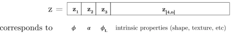
𝜙1 𝛼1 𝛼 𝜙L1 𝜙L z_[4,n]

z =

Output

first sample in batch x

from encoder

to encoder

intrinsic properties (shape, texture, etc)

same as output for x1

z_[4,n] z₃

z₂ z₁

later samples in batch x

[4,n]

z₃ z₂ z₁

unique for each xi _{in batch}

zero error signal for clamped outputs

zero error signal for clamped outputs

error signal from decoder

∇z

= z

- mean z

Backpropagation

Backpropagation with

invariance targeting

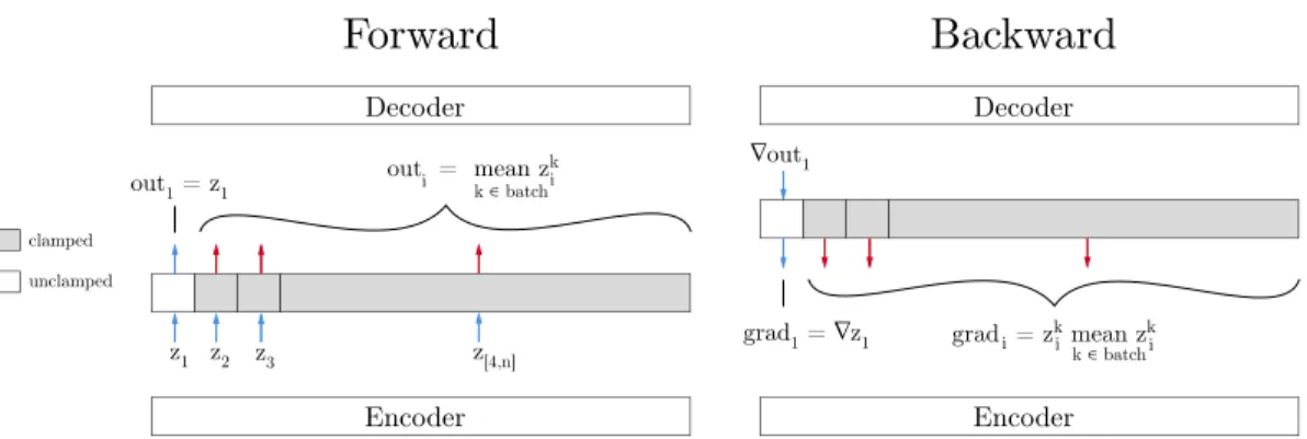
Caption: Training on a minibatch in which only

_{𝜙, the azimuth angle of the face,}

changes.

During the forward step, the output from each component z_k != z_1 of the

encoder is forced to be the same for each sample in the batch. This reflects the fact

that the generating variables of the image which correspond to the desired values of

these latents are unchanged throughout the batch. By holding these outputs

constant throughout the batch, z_1 is forced to explain all the variance within the

batch, i.e. the full range of changes to the image caused by changing

_𝜙.

During the backward step, backpropagation of gradients happens only through the latent

z_1, with gradients for z_k != z_1 set to zero. This corresponds with the clamped

output from those latents throughout the batch.

Caption:

_{In order to directly enforce invariance of the latents corresponding to}

properties of the image which do not change within a given batch, we calculate

gradients for the z_k != z_1 which move them towards the mean of each

invariant latent over the batch. This is equivalent to regularizing the

Figure 2: Structure of the representation vector. φ is the azimuth of the face, α is the elevation of the face with respect to the camera, and φL is the azimuth of the light source.

2

Related Work

As mentioned previously, a number of generative models have been proposed in the litera-ture to obtain abstract visual representations. Unlike most RBM-based models [8, 19, 14], our approach is trained using back-propagation with objective function consisting of data reconstruction and the variational bound.

Relatively recently, Kingma et al. [10] proposed the SGVB algorithm to learn generative models with continuous latent variables. In this work, a feed-forward neural network (en-coder) is used to approximate the posterior distribution and a decoder network serves to enable stochastic reconstruction of observations. In order to handle fine-grained geometry of faces, we work with relatively large scale images (150 × 150 pixels). Our approach extends and applies the SGVB algorithm to jointly train and utilize many layers of convolution and convolution operators for the encoder and decoder network respectively. The de-coder network is a function that transform a compact graphics code ( 200 dimensions) to a 150 × 150 image. We propose using unpooling (nearest neighbor sampling) followed by convolution to handle the massive increase in dimensionality with a manageable number of parameters.

Recently, [6] proposed using CNNs to generate images given object-specific parameters in a supervised setting. As their approach requires ground-truth labels for the graphics code layer, it cannot be directly applied to image interpretation tasks. Our work is similar to Ranzato et al. [18], whose work was amongst the first to use a generic encoder-decoder architecture for feature learning. However, in comparison to our proposal their model was trained layer-wise, the intermediate representations were not disentangled like a graphics

code, and their approach does not use the variational auto-encoder loss to approximate the

posterior distribution. Our work is also similar in spirit to [20], but in comparison our model does not assume a Lambertian reflectance model and implicitly constructs the 3D representations. Another piece of related work is Desjardins et al. [5], who used a spike and slab prior to factorize representations in a generative deep network.

In comparison to existing approaches, it is important to note that our encoder network produces the interpretable and disentangled representations necessary to learn a meaningful 3D graphics engine. A number of inverse-graphics inspired methods have recently been proposed in the literature [15]. However, most such methods rely on hand-crafted rendering engines. The exception to this is work by Hinton et al. [9] and Tieleman [21] on transforming

autoencoders which use a domain-specific decoder to reconstruct input images. Our work

is similar in spirit to these works but has some key differences: (a) It uses a very generic convolutional architecture in the encoder and decoder networks to enable efficient learning on large datasets and image sizes; (b) it can handle single static frames as opposed to pair of images required in [9]; and (c) it is generative.

3

Model

As shown in Figure 1, the basic structure of the Deep Convolutional Inverse Graphics Net-work (DC-IGN) consists of two parts: an encoder netNet-work which captures a distribution over

graphics codes Z given data x and a decoder network which learns a conditional distribution

to produce an approximation ˆx given Z. Z can be a disentangled representation containing

a factored set of latent variables zi ∈ Z such as pose, light and shape. This is important

Forward

Backward

Figure 3: Training on a minibatch in which only φ, the azimuth angle of the

face, changes. During the forward step, the output from each component zi 6= z1 of the

encoder is altered to be the same for each sample in the batch. This reflects the fact that the generating variables of the image (e.g. the identity of the face) which correspond to the desired values of these latents are unchanged throughout the batch. By holding these outputs constant throughout the batch, the single neuron z1 is forced to explain all the

variance within the batch, i.e. the full range of changes to the image caused by changing φ. During the backward step z1 is the only neuron which receives a gradient signal from the

attempted reconstruction, and all zi 6= z1 receive a signal which nudges them to be closer

to their respective averages over the batch. During the complete training process, after this batch, another batch is selected at random; it likewise contains variations of only one of

φ, α, φL, intrinsic; all neurons which do not correspond to the selected latent are clamped;

and the training proceeds.

in learning a meaningful approximation of a 3D graphics engine and helps tease apart the generalization capability of the model with respect to different types of transformations. Let us denote the encoder output of DC-IGN to be ye= encoder(x). The encoder output

is used to parametrize the variational approximation Q(zi|ye), where Q is chosen to be a

multivariate normal distribution. There are two reasons for using this parametrization: (1) Gradients of samples with respect to parameters θ of Q can be easily obtained using the reparametrization trick proposed in [10], and (2) Various statistical shape models trained on 3D scanner data such as faces have the same multivariate normal latent distribution [17]. Given that model parameters We connect ye and zi, the distribution parameters

θ = (µzi, Σzi) and latents Z can then be expressed as:

µz= Weye, Σz= diag(exp(Weye)) (1)

∀i, zi∼ N (µzi, Σzi) (2)

We present a novel training procedure which allows networks to be trained to have disen-tangled and interpretable representations.

3.1 Training with Specific Transformations

The main goal of this work is to learn a representation of the data which consists of disen-tangled and semantically interpretable latent variables. We would like only a small subset of the latent variables to change for sequences of inputs corresponding to real-world events. One natural choice of target representation for information about scenes is that already designed for use in graphics engines. If we can deconstruct a face image by splitting it into variables for pose, light, and shape, we can trivially represent the same transformations that these variables are used for in graphics applications. Figure 2 depicts the representation which we will attempt to learn.

With this goal in mind, we perform a training procedure which directly targets this definition of disentanglement. We organize our data into mini-batches corresponding to changes in only a single scene variable (azimuth angle, elevation angle, azimuth angle of the light

(a) (b)

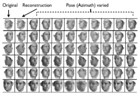
Figure 4: Manipulating light and elevation variables: Qualitative results showing the generalization capability of the learned DC-IGN decoder to re-render a single input image with different pose directions. (a) We change the latent zlight smoothly leaving all 199

other latents unchanged. (b) We change the latent zelevationsmoothly leaving all 199 other

latents unchanged.

source); these are transformations which might occur in the real world. We will term these the extrinsic variables, and they are represented by the components z1,2,3 of the encoding.

We also generate mini-batches in which the three extrinsic scene variables are held fixed but all other properties of the face change. That is, these batches consist of many different faces under the same viewing conditions and pose. These intrinsic properties of the model, which describe identity, shape, expression, etc., are represented by the remainder of the latent variables z[4,200]. These mini-batches varying intrinsic properties are interspersed

stochastically with those varying the extrinsic properties.

We train this representation using SGVB, but we make some key adjustments to the outputs of the encoder and the gradients which train it. The procedure (Figure 3) is as follows.

1. Select at random a latent variable ztrain which we wish to correspond to one of

{azimuth angle, elevation angle, azimuth of light source, intrinsic properties}. 2. Select at random a mini-batch in which that only that variable changes.

3. Show the network each example in the minibatch and capture its latent represen-tation for that example zk_.

4. Calculate the average of those representation vectors over the entire batch. 5. Before putting the encoder’s output into the decoder, replace the values zi6= ztrain

with their averages over the entire batch. These outputs are “clamped”. 6. Calculate reconstruction error and backpropagate as per SGVB in the decoder. 7. Replace the gradients for the latents zi 6= ztrain (the clamped neurons) with their

difference from the mean (see Section 3.2). The gradient at ztrainis passed through

unchanged.

8. Continue backpropagation through the encoder using the modified gradient. Since the intrinsic representation is much higher-dimensional than the extrinsic ones, it requires more training. Accordingly we select the type of batch to use in a ratio of about 1:1:1:10, azimuth : elevation : lighting : intrinsic; we arrived at this ratio after extensive testing, and it works well for both of our datasets.

This training procedure works to train both the encoder and decoder to represent certain properties of the data in a specific neuron. By clamping the output of all but one of the neurons, we force the decoder to recreate all the variation in that batch using only the changes in that one neuron’s value. By clamping the gradients, we train the encoder to put all the information about the variations in the batch into one output neuron.

This training method leads to networks whose latent variables have a strong equivariance with the corresponding generating parameters, as shown in Figure 6. This allows the value

of the true generating parameter (e.g. the true angle of the face) to be trivially extracted from the encoder.

3.2 Invariance Targeting

By training with only one transformation at a time, we are encouraging certain neurons to contain specific information; this is equivariance. But we also wish to explicitly discourage them from having other information; that is, we want them to be invariant to other trans-formations. Since our mini-batches of training data consist of only one transformation per batch, then this goal corresponds to having all but one of the output neurons of the encoder give the same output for every image in the batch.

To encourage this property of the DC-IGN, we train all the neurons which correspond to the inactive transformations with an error gradient equal to their difference from the mean. It is simplest to think about this gradient as acting on the set of subvectors zinactive from

the encoder for each input in the batch. Each of these zinactive’s will be pointing to a

close-together but not identical point in a high-dimensional space; the invariance training signal will push them all closer together. We don’t care where they are; the network can represent the face shown in this batch however it likes. We only care that the network always represents it as still being the same face, no matter which way it’s facing. This regularizing force needs to be scaled to be much smaller than the true training signal, otherwise it can overwhelm the reconstruction goal. Empirically, a factor of 1/100 works well.

4

Experiments

Figure 5: Manipulating azimuth

(pose) variables: Qualitative results showing the generalization capability of the learnt DC-IGN decoder to render original static image with different az-imuth (pose) directions. The latent neu-ron zazimuthis changed to random values

but all other latents are clamped. We trained our model on about 12,000 batches

of faces generated from a 3D face model ob-tained from Paysan et al. [17], where each batch consists of 20 faces with random variations on face identity variables (shape/texture), pose, or lighting. We used the rmsprop [22] learning algo-rithm during training and set the meta learning rate equal to 0.0005, the momentum decay to 0.1 and weight decay to 0.01.

To ensure that these techniques work on other types of data, we also trained networks to per-form reconstruction on images of widely varied 3D chairs from many perspectives derived from the Pascal Visual Object Classes dataset as ex-tracted by Aubry et al. [16, 1]. This task tests the ability of the DC-IGN to learn a rendering function for a dataset with high variation be-tween the elements of the set; the chairs vary from office chairs to wicker to modern designs, and viewpoints span 360 degrees and two ele-vations. These networks were trained with the same methods and parameters as the ones above.

4.1 3D Face Dataset

The decoder network learns an approximate rendering engine as shown in Figures (4,7). Given a static test image, the encoder network produces the latents Z depicting scene variables such as light, pose, shape etc. Similar to an off-the-shelf rendering engine, we can independently control these to generate new images with the decoder. For example, as shown in Figure 7, given the original test image, we can vary the lighting of an image by keeping all the other latents constant and varying zlight. It is perhaps surprising that the

fully-trained decoder network is able to function as a 3D rendering engine.

(a) (b) (c)

Figure 6: Generalization of decoder to render images in novel viewpoints and

lighting conditions: We generated several datasets by varying light, azimuth and

eleva-tion, and tested the invariance properties of DC-IGN’s representation Z. We show quan-titative performance on three network configurations as described in section 4.1. (a,b,c) All DC-IGN encoder networks reasonably predicts transformations from static test images. Interestingly, as seen in (a), the encoder network seems to have learnt a switch node to separately process azimuth on left and right profile side of the face.

We also quantitatively illustrate the network’s ability to represent pose and light on a smooth linear manifold as shown in Figure 6, which directly demonstrates our training algorithm’s ability to disentangle complex transformations. In these plots, the inferred and ground-truth transformation values are plotted for a random subset of the test set. Interestingly, as shown in Figure 6(a), the encoder net-work’s representation of azimuth has a discontinuity at 0◦ (facing straight forward).

Figure 7: Entangled ver-sus disentangled repre-sentations. First column: Original images. Second column: transformed image using DC-IGN. Third col-umn: transformed image us-ing normally-trained network.

4.1.1 Comparison with Entangled Representations

To explore how much of a difference the DC-IGN training procedure makes, we compare the novel-view reconstruction performance of networks with entangled representations (line) versus disentangled representations (DC-IGN). The base-line network is identical in every way to the DC-IGN, but was trained with SGVB without using our proposed training pro-cedure. As in Figure 4, we feed each network a single input image, then attempt to use the decoder to re-render this image at different azimuth angles. To do this, we first must figure out which latent of the entangled representation most closely corresponds to the azimuth. This we do rather simply. First, we encode all images in an azimuth-varied batch using the baseline’s encoder. Then we calculate the variance of each of the latents over this batch. The latent with the largest vari-ance is then the one most closely associated with the azimuth of the face, and we will call it zazimuth. Once that is found,

the latent zazimuth is varied for both the models to render a

novel view of the face given a single image of that face. Figure 7 shows that explicit disentanglement is critical for novel-view reconstruction.

4.2 Chair Dataset

We performed a similar set of experiments on the 3D chairs dataset described above. This dataset contains still images rendered from 3D CAD models of 1357 different chairs, each model skinned with the photographic texture of the real chair. Each of these models is rendered in 60 different poses; at each of two elevations, there are 30 images taken from 360 degrees around the model. We used approximately 1200 of these chairs in the training set and the remaining 150 in the test set; as such, the networks had never seen the chairs in the test set from any angle, so the tests explore the networks’ ability to generalize to arbitrary

(a)

(b)

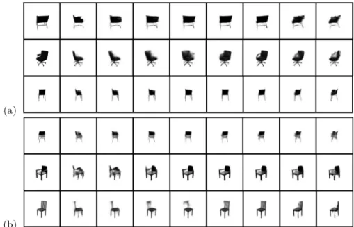
Figure 8: Manipulating rotation: Each row was generated by encoding the input image (leftmost) with the encoder, then changing the value of a single latent and putting this modified encoding through the decoder. The network has never seen these chairs before at any orientation. (a) Some positive examples. Note that the DC-IGN is making a conjecture about any components of the chair it cannot see; in particular, it guesses that the chair in the top row has arms, because it can’t see that it doesn’t. (b) Examples in which the network extrapolates to new viewpoints less accurately.

chairs. We resized the images to 150 × 150 pixels and made them grayscale to match our face dataset.

We trained these networks with the azimuth (flat rotation) of the chair as a disentangled vari-able represented by a single node z1; all other variation between images is undifferentiated

and represented by z[2,200]. The DC-IGN network succeeded in achieving a mean-squared

error (MSE) of reconstruction of 2.7722 × 10−4 on the test set. Each image has grayscale values in the range [0, 1] and is 150 × 150 pixels.

In Figure 8 we have included examples of the network’s ability to re-render previously-unseen chairs at different angles given a single image. For some chairs it is able to render fairly smooth transitions, showing the chair at many intermediate poses, while for others it seems to only capture a sort of “keyframes” representation, only having distinct outputs for a few angles. Interestingly, the task of rotating a chair seen only from one angle requires speculation about unseen components; the chair might have arms, or not; a curved seat or a flat one; etc.

5

Discussion

We have shown that it is possible to train a deep convolutional inverse graphics network with a fairly disentangled, interpretable graphics code layer representation from static images. By utilizing a deep convolution and de-convolution architecture within a variational autoencoder formulation, our model can be trained end-to-end using back-propagation on the stochastic variational objective function [10]. We proposed a training procedure to force the network to learn disentangled and interpretable representations. Using 3D face and chair analysis as a working example, we have demonstrated the invariant and equivariant characteristics of the learned representations.

Acknowledgements: We thank Thomas Vetter for access to the Basel face model. We are

grateful for support from the MIT Center for Brains, Minds, and Machines (CBMM). We also thank Geoffrey Hinton and Ilker Yildrim for helpful feedback and discussions.

References

[1] M. Aubry, D. Maturana, A. Efros, B. Russell, and J. Sivic. Seeing 3d chairs: exemplar part-based 2d-3d alignment using a large dataset of cad models. In CVPR, 2014.

[2] Y. Bengio. Learning deep architectures for ai. Foundations and trends in Machine Learning,R

2(1):1–127, 2009.

[3] Y. Bengio, A. Courville, and P. Vincent. Representation learning: A review and new perspec-tives. Pattern Analysis and Machine Intelligence, IEEE Transactions on, 35(8):1798–1828, 2013.

[4] T. Cohen and M. Welling. Learning the irreducible representations of commutative lie groups.

arXiv preprint arXiv:1402.4437, 2014.

[5] G. Desjardins, A. Courville, and Y. Bengio. Disentangling factors of variation via generative entangling. arXiv preprint arXiv:1210.5474, 2012.

[6] A. Dosovitskiy, J. Springenberg, and T. Brox. Learning to generate chairs with convolutional neural networks. arXiv:1411.5928, 2015.

[7] I. Goodfellow, H. Lee, Q. V. Le, A. Saxe, and A. Y. Ng. Measuring invariances in deep networks. In Advances in neural information processing systems, pages 646–654, 2009. [8] G. Hinton, S. Osindero, and Y.-W. Teh. A fast learning algorithm for deep belief nets. Neural

computation, 18(7):1527–1554, 2006.

[9] G. E. Hinton, A. Krizhevsky, and S. D. Wang. Transforming auto-encoders. In Artificial Neural

Networks and Machine Learning–ICANN 2011, pages 44–51. Springer, 2011.

[10] D. P. Kingma and M. Welling. Auto-encoding variational bayes. arXiv preprint arXiv:1312.6114, 2013.

[11] T. D. Kulkarni, P. Kohli, J. B. Tenenbaum, and V. Mansinghka. Picture: A probabilistic pro-gramming language for scene perception. In Proceedings of the IEEE Conference on Computer

Vision and Pattern Recognition, pages 4390–4399, 2015.

[12] T. D. Kulkarni, V. K. Mansinghka, P. Kohli, and J. B. Tenenbaum. Inverse graphics with probabilistic cad models. arXiv preprint arXiv:1407.1339, 2014.

[13] Y. LeCun and Y. Bengio. Convolutional networks for images, speech, and time series. The

handbook of brain theory and neural networks, 3361, 1995.

[14] H. Lee, R. Grosse, R. Ranganath, and A. Y. Ng. Convolutional deep belief networks for scal-able unsupervised learning of hierarchical representations. In Proceedings of the 26th Annual

International Conference on Machine Learning, pages 609–616. ACM, 2009.

[15] V. Mansinghka, T. D. Kulkarni, Y. N. Perov, and J. Tenenbaum. Approximate bayesian image interpretation using generative probabilistic graphics programs. In Advances in Neural

Information Processing Systems, pages 1520–1528, 2013.

[16] R. Mottaghi, X. Chen, X. Liu, N.-G. Cho, S.-W. Lee, S. Fidler, R. Urtasun, and A. Yuille. The role of context for object detection and semantic segmentation in the wild. In IEEE Conference

on Computer Vision and Pattern Recognition (CVPR), 2014.

[17] P. Paysan, R. Knothe, B. Amberg, S. Romdhani, and T. Vetter. A 3d face model for pose and illumination invariant face recognition. Genova, Italy, 2009. IEEE.

[18] M. Ranzato, F. J. Huang, Y.-L. Boureau, and Y. LeCun. Unsupervised learning of invariant feature hierarchies with applications to object recognition. In Computer Vision and Pattern

Recognition, 2007. CVPR’07. IEEE Conference on, pages 1–8. IEEE, 2007.

[19] R. Salakhutdinov and G. E. Hinton. Deep boltzmann machines. In International Conference

on Artificial Intelligence and Statistics, pages 448–455, 2009.

[20] Y. Tang, R. Salakhutdinov, and G. Hinton. Deep lambertian networks. arXiv preprint arXiv:1206.6445, 2012.

[21] T. Tieleman. Optimizing Neural Networks that Generate Images. PhD thesis, University of Toronto, 2014.

[22] T. Tieleman and G. Hinton. Lecture 6.5 - rmsprop, coursera: Neural networks for machine learning. 2012.

[23] P. Vincent, H. Larochelle, I. Lajoie, Y. Bengio, and P.-A. Manzagol. Stacked denoising au-toencoders: Learning useful representations in a deep network with a local denoising criterion.