Demonstration System for a Low-Power
Classification Processor
by
David J. Rowe
Submitted to the Department of Electrical Engineering and Computer
Science
in partial fulfillment of the requirements for the degree of
Master of Science in Electrical Engineering
at the
MASSACHUSETTS INSTITUTE OF TECHNOLOGY
February 2000
@
David J. Rowe, MM. All rights reserved.
The author hereby grants to MIT permission to reproduce and
distribute publicly paper and electronic copies of this thesis document
in whole or in part.
A uthor
...
Department of Electrical Engineering and Computer Science
February 4, 2000
C ertified by ... /... I...Anantha Chandrakasan
Associate Professor
Thesis Supervisor
Accepted by ...
USETTS INSTITUTE -
Arthur
C.
Sh
ECHNOLOGY
Chairman, Department Committee on Graduate Stud en s MASSACH
OFT
Demonstration System for a Low-Power Classification
Processor
by
David J. Rowe
Submitted to the Department of Electrical Engineering and Computer Science on February 4, 2000, in partial fulfillment of the
requirements for the degree of Master of Science in Electrical Engineering
Abstract
The purpose of this thesis was to develop a self-contained digital system using an ultra low power classification processor for biomedical sensing applications. The initial application for the system was heartbeat detection.
The system consists of an analog input from an amplified microphone, a digital test data input, a programming interface to the processor, and a data output interface. The completed system demonstrates that a useful digital signal processing algorithm can be implemented at the desired low power constraints. Further work will show that these power levels can be achieved using an ambient vibrational source.
Thesis Supervisor: Anantha Chandrakasan Title: Associate Professor
Acknowledgments
First and foremost, I would like to thank Professor Anantha Chandrakasan for allow-ing me to work on this project. His endurallow-ing patience and encouragement have been greatly appreciated during the course of this project. I am inspired by the example of his success, but more-so by his dedication to his students. I cannot thank him enough for his support.
This thesis is merely a continuation of the innovation by Raj Amirtharajah. All aspects of the technical ingenuity within this thesis can be entirely attributed to Raj. I very much appreciated the extra time he spent answering questions and helping out in tough situations. I would like to thank him for putting up with my incessant phone calls and emails. I feel privileged to have had to opportunity to work on his project. The technical and philosophical advice of Manish Bhardwaj and Jim Goodman has been a live-saver during the course of this project. Their modesty would not permit them to recognize their contribution, but their help has been unmeasurable. I would also like to thank the other members of Anantha's group for making the lab a friendly and welcoming place to work, Alice Wang, Rex Min, Eugene Shih, Seong-Hwan Cho, Amit Sinha, Travis Furrer, Charatpong (Boo) Chotigavanich, Wendi Heinzelman, and Vadim Gutnik. A great many thanks to Margaret Flaherty for her assistance during my time in the group.
My most meaningful experience during my tenure at MIT has been being a TA
for 6.111. I have learned more through a year of teaching than in four years of undergraduate studies. Thanks to Professor Donald Troxel and Professor James Kirtley for giving me the opportunity to work with them in 6.111. I would also like to thank my fellow TA's, Everest Huang, Rob Jagnow, Alex Ihler, Theresa Huang,
Josef Brandriss, Jessica Forbess, and Ali Tariq. Thank you also to Danny Seth and Syed Alam for being good friends and classmates.
The individuals who have inspired me the most during my academic career are Pro-fessor Hamid Nawab and ProPro-fessor Thomas Kincaid from Boston University. Their devotion to teaching is unsurpassed. They are very much responsible for the success
I have obtained.
Despite my absence from the usual circle of friends during my thesis work, I very much appreciate the support and friendship of my close friends, Jack Livingston, John Arrigo, Jen Saleem, Man Leung, Vishal Goklani, Mike Chipolone, and Vince Leslie.
Without the love and support of my family, my achievements at MIT and BU could never have been accomplished. My parents, Jack and Linda Rowe, my grandmother, Mary Ruth Ross, my brother, Stephen Rowe, and my cousin, Tim Gumto, have be an ever present source of love, support, and encouragement. I can never thank them enough for all they have done for me. I promise to continue to do my best to make them proud. I love you all very much.
Finally, I would like to thank my love, Kelly Dugan, for her warmth, compassion, and love. She has been there at every moment when I needed her. I can only hope that I will someday be able to repay her for all she has done for me. I love you, Kelly.
Contents
1 Introduction 15 1.1 Background . . . . 16 1.1.1 Matched Filtering . . . . 16 1.1.2 Distributed Arithmetic . . . . 18 1.2 Overview . . . . 202 SensorDSP Chip Architecture 23 2.1 Distributed Arithmetic Matched Filter . . . . 24
2.2 Non-Linear/Short Linear Filter . . . . 27
2.3 Micro-controller Unit . . . . 27
3 System Design Description 31 3.1 Programming Interface . . . . 32
3.1.1 JTAG Interface . . . . 32
3.1.2 Programming Interface Description . . . . 34
3.2 Analog Sensor Interface . . . . 40
3.3 Heartbeat Indicator. . . . .. . . . . 42
3.4 Clock Generation . . . . 43
3.5 Power Measurement . . . . 46
3.6 Battery Vs. External Supply . . . . 48
3.7 Test Ports . . . . 48
4.1 Compiling Program Data .5
4.2 Running the System . . . . 56
4.2.1 Initial Settings . . . . 56
4.2.2 Operating the System . . . . 57
4.3 Analog Signal Requirements . . . . 57
4.3.1 Using the ARL Sensor . . . . 58
4.4 Test Data Input . . . . 58
4.5 Extracting Data . . . . 59
4.5.1 Heartbeat Detection Indicator . . . . 59
4.5.2 Hexadecimal Display . . . . 60
4.5.3 Using the Test Ports . . . . 60
4.6 Additional Features . . . . 60
4.6.1 Multiple Programs . . . . 60
4.6.2 Changing Clock Speeds. . . . . 61
4.7 Troubleshooting . . . . 61
5 Conclusions 63 A SensorDSP Chip Pinouts 65 B Sensor DSP Microcontroller Assembly Language [1] 67 B.1 Instruction Set Overview . . . . 67
B.2 Registers and Other State . . . . 69
B.3 Instruction Descriptions . . . . 70 B.3.1 RTL Description . . . . 71 B.3.2 Miscellaneous Instructions . . . . 72 B.3.3 Arithmetic Instructions . . . . 72 B.3.4 Arithmetic Macros . . . . 74 B.3.5 Relational Macros . . . . 75
B.3.6 Logical and Shift Instructions . . . . 76 52
B.3.8 Memory Instructions . . . .
B.3.9 Filter Interface Instructions . . B.3.10 Unused Opcodes . . . . B.3.11 Miscellaneous Reserved Words . B.4 Example Program: Fibonacci Numbers
C Sensor DSP Nonlinear/Short Linear Fi C.1 Registers . . . . C.2 Instruction Descriptions . . . . C.2.1 SAC Instructions . . . . C.2.2 MAC Instructions . . . . C.2.3 LSU Instructions . . . . . . . . . . . . . . . . . . . . . . . .
Ilter Assembly Language [1]
. . . . . . . . . . . . . . . . . . . .
D SensorDSP Sample Microcode
D.1 Micro-controller Heart Detection Code D.2 NLSL SAC Heart Detection Code . . . D.3 NLSL MAC Heart Detection Code . .
D.4 NLSL LSU Heart Detection Code . . .
80 81 82 82 83 85 85 86 86 88 89 91 91 98 98 98
List of Figures
1-1 Matched Filter Template . . . . 16
1-2 Typical Matched Filter Result . . . . 17
1-3 Heartbeat Waveform and Matched Filter Result . . . . 17
1-4 Distributed Arithmetic ROM and Accumulator Structure [1, p. 119] . 19 2-1 Classification and Signal Processing Block Diagram [1, p. 128] . . . . 24
2-2 Signal Processing Chip Architecture [1, p. 128] . . . . 24
2-3 Linear Filter Implementation Architecture [1, p. 130] . . . . 25
2-4 DA Unit Shift Register Implementation [1, p. 131] . . . . 26
2-5 NLSL Filter Implementation Architecture [1, p. 131] . . . . 28
2-6 Micro-controller Architecture [1, p. 132] . . . . 28
3-1 System Block Diagram . . . . 31
3-2 JTAG TAP State Diagram . . . . 33
3-3 JTAG Controller State Diagram . . . . 35
3-4 Programming Controller FSM State Diagram . . . . 36
3-5 Programming Instruction Formats . . . . 39
3-6 Programming Interface Block Diagram . . . . 40
3-7 A/D Converter Timing . . . . 41
3-8 Analog Sensor Interface Block Diagram . . . . 42
3-9 Heartbeat Indicator Block Diagram . . . . 44
3-10 Read Trigger Timing . . . . 45
3-11 Clock Generation Circuitry . . . . 46
3-13 Power Regulation Schematic . . . .4
3-14 Test Point Pin Diagram . . . .
4-1 SensorDSP System Board Floor-plan . . . .
5-1 SensorDSP Demonstration System Board . . . .
A-1 SensorDSP Chip Footprint (Top View) [1] . . . . A-2 SensorDSP Chip Footprint (Bottom View) [1] . . . .
B-i Sensor DSP microcontroller architecture. . . . .
C-1 Short linear and nonlinear filter implementation architecture. .
. . . . 49 53 64 65 65 68 86 48
List of Tables
3.1 3.2 3.3 3.4 3.5TAP Instruction Words . . . . Program Instruction Bit-sizes . . . . Truncation and Bit-width Configuration Settings SensorDSP Output Bus Selection . . . . Test Port Signals . . . .
35 37 38 43 49 54 58 66 67 69 70
4.1 Component Reference Designations . . . . 4.2 ARL Sensor Gain Settings . . . .
A.1 SensorDSP Chip Pinout . . . .
B.1 Microcontroller instruction types. . . . . B.2 Microcontroller registers. . . . . B.3 Condition code register field specifiers for conditional jumps.
B.4 Configuration state bit specifiers for configuration instructions. ... 70
B.5 Microcontroller instruction syntax and RTL level description . . . . . 71
B.6 Arithmetic instructions and opcodes. . . . . 72
B.7 Arithmetic instructions and opcodes. . . . . 72
B.8 Arithmetic macros and implementations. . . . . 74
B.9 Relational macros and implementations. . . . . 75
B.10 Logical and shift instructions and opcodes. . . . . 77
B.11 Control flow instructions and opcodes. . . . . 79
B.12 Memory instructions and opcodes. . . . . 80
B.14 Configuration state specifiers and codes. . . . . 82
B.15 Unused opcodes. . . . . 82
B.16 Microcontroller instruction types. . . . . 83
C.1 NLSL Unit registers. . . . . 86
C.2 SAC Unit instructions and opcodes. . . . . 87
C.3 MAC Unit instructions and opcodes. . . . . 88
Chapter 1
Introduction
In recent years, there has been an ever expanding demand for portable devices for such applications as wireless communication and hand-held computers. These sys-tems rely heavily on batteries as their source of energy. Investigation of alternative sources for power generation and storage is a growing endeavor as the limits of device physics are reached with increasing clock rates and lower supply voltages. A potential alternative power generating technique is to convert ambient vibrational energy into useful electrical energy as proposed by Amirtharajah [1][2][3].
One application of such a system is biomedical sensing, for example, heartbeat monitoring. The feasibility of such a system imposes certain constraints on the type of application. In order to attain the low power consumption required by the limitations of the ambient energy converter, the digital system must employ a variety of low power VLSI (Very Large Scale Integration) design techniques. Many of these techniques present a trade-off between speed and power dissipation. A human heartbeat can be measured with a microphone, and be converted into a digital signal that can be analyzed and classified with a digital signal processor (DSP). The classification processor developed by Amirtharajah takes advantage of a multitude of low-power design techniques to implement a heartbeat detection algorithm, while consuming approximately 500nW at 1.5V with a 1 kHz clock frequency.
1.1
Background
1.1.1
Matched Filtering
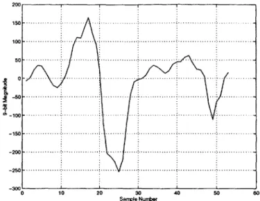
200 2100 .. . mp. N. .b. . -200 L -0 10 20 30 40 60 0 Sample NufferFigure 1-1: Matched Filter Template
Matched filtering is a signal processing technique used to detect a specific pattern in the input signal. A system is designed to have an impulse response, h[k], that is a replica of the desired input signal [4]. A typical matched filter template for a human heartbeat is shown in Figure 1-1. The result of the matched filtering process is a signal, y[k], as shown in Figure 1-2. The signal, y[k], has several characteristics that can be measured, ranked, and classified. [1, pp. 105-125]
These signal features are summarized below:
1. peak correlation output value
2. first valley after peak correlation
3. first valley before peak correlation
4. first peak after peak correlation
5. first peak before peak correlation 6. matched filter output energy
3 2.5 2 1.5 0.5 0 -0.5 -1 -1.5 20 40 60 Sample Number 80 100 120
Figure 1-2: Typical Matched Filter Result
Digitized Heartbeat Data
---. --- .-- ..--- ...---- --- .. .-. . .. - ... .---- --- -.--- .---- ---- ---- --- --- -- - - - -- -- ---- -. -- -- --- -- -.. -. .- .... .-- --- - --.. -- ---.-- 0 500 1000 1500 2000 2500 3000 Sample Number (fs = 112.5 Hz) 4~- C -ti n R l 3500 4000 45 x 10 W orm andsR 8 6 --- --- - . . .. .--- --- ---. ... .. --- -.- -...-- --- --- --- - ..--- ---4 ... ... . ... ... ... . a ... . ... ..w... 0 -- - - - . ---...--- -0 500 1000 1500 2000 2500 3000 3500 4000 4500 Sample Number
Figure 1-3: Heartbeat Waveform and Matched Filter Result
Figure 1-3 shows a heartbeat signal recorded via an analog acoustic sensor as well
as the resultant signal when the heartbeat is passed through the matched filter.
-..-..- ...- ..- ..- ..-. .-. .- .-. -. . . -. .-.. .-. -. . -. -. . .- .-. -. -.-. --.. . -. -. . -. .. .- . .. .. ... .. .. .. . .. .. ..--. ... .. ...-.. -. ... ...-.- -.-.-.-. .- ..- ..- . --- .. --- --- .. ...- - -- .----.-.-.----..----.--- -- . .... ... ..-.- ....---- ....---- -- -- --- . ... -. ...--- -. -. -- -. ...-.-.-..-. ... ...-. ...- . -.. . . ...---. .... -. ...-. -. .. .. -- -.-- ---. . .... ... .-- -.- -.-.-- - .- .-- .-. ---. --- .--- -- -- - ---.. --- - -- ---- -- ---.. --. .... -. --- --- --- --- -. -- --- -. -. --. -. -- - -.-- .. . ..-- - -.-.- .. -- - - -- - - ----. 50 0 -50
I
luux 10'' Typical Matched Filter Result
1.1.2
Distributed Arithmetic
Distributed Arithmetic (DA) is a bit-serial operation that computes the inner prod-uct of two vectors (one of which is a constant) in parallel without the use of a mul-tiplier [5][6]. The constant vector, with regards to linear filtering, is the impulse response of the filter. The distributed arithmetic calculation is implemented using a read-only memory (ROM) lookup table, an input shift register, and an output accu-mulator. An advantage of the distributed arithmetic approach, is that an approximate result can be obtained using a lower quantization of the input signal. Using a smaller bit-width yields a trade-off between power reduction and detection accuracy.
Figure 1-4 show a detailed example of a distributed arithmetic computation. The structure shown computes the dot product of a 4-element vector X and a constant vector A. All 16 possible linear combinations of the constant vector elements (Ai) are stored in the ROM. The variable vector X is repackaged to form the ROM address most significant bit first. We have assumed that the Xi elements are 4-bits 2's comple-ment (bit 3 is the sign bit) binary numbers. Every clock cycle, the RESULT register adds 2x its previous value (reset to zero) to the current ROM contents. Moreover, after each cycle the 4 registers that hold the four elements of the X vector are shifted to the right. The sign timing pulse, T, is activated when the ROM is addressed
by bit 3 of the vector elements (sign). In this case, the adder subtracts the current
ROM contents from the accumulator state. After 4 cycles, (4 is the bit-width of the Xi elements) the dot product has been produced within the RESULT register [1, p.
X0
I
X01 X02 X03 lo xli Ixi xi X1 X11 12 X1/ X20 X21 X22 X23 X30 X31 X32 X33 0 x we 0 AO Al A1+AO A2 A2+AO A2+A A2+A1+AO A3 A3+AO A3+Al A3+A1+AO A3+A2 A3+A2+AO A3+A2+A1 A3+A2+A+A Tsx2
RESULTFigure 1-4: Distributed Arithmetic ROM and Accumulator Structure [1, p. 119]
1.2
Overview
The goal of this project was to design and develop a complete, self-enclosed system that uses an ultra low power digital signal processor (DSP) to implement a heartbeat detection algorithm. The heart of the system is a DSP designed by Amirtharajah [1], herein referred to as the SensorDSP chip. A subsequent goal of the project is to prove that a useful digital signal processing system can be implemented at power levels low enough to use ambient vibrational energy as the source of power. The following is a
list of requirements for the system:
1. Programming Interface - The SensorDSP chip is programmed using a serial boundary-scan register. Matched filter coefficients, micro-controller instruc-tions, and other control words are generated using a computer program and then stored on a programmable read-only memory (PROM). The programming interface transmits data from the PROM into the SensorDSP chip.
2. Analog Sensor Interface - Provided with the SensorDSP system is a an analog sensor that the patient would wear on the neck or chest. The analog sensor was provided by the Army Research Laboratory. The analog sensor interface samples data from the analog sensor and sends the data serially into the SensorDSP chip.
3. Test Data Input - In addition to an analog data input, the system allows for test data to be stored into a PROM. This data can be serially input into the SensorDSP instead of data from the analog sensor. Although this feature is primarily meant for debugging purposes, it is also useful when devising al-gorithms for other applications since the alal-gorithms can be tested with known input data.
4. Detection Logic -Due to a limited number of pins the chip has a limited data output capability. The SensorDSP has an 8 to 1 multiplexed 12-bit output bus. The detection logic controls the select inputs to the multiplexer and reads
emitting diode) display, or in the case of heartbeat detection, a single LED is flashed when a detection occurs.
5. Power Measurement/Monitoring - The system provides two methods of measuring the power consumption of the SensorDSP chip. First, a connection on the circuit board is allocated for an external ammeter to be connected for an accurate power measurement. Second, a power measurement circuit on the board provides a bar-graph display of the power consumption.
6. Clock Generation - Although the heartbeat detection system operates at a fixed optimal system clock frequency, the SensorDSP system provides the capability to operate at a wide range of speeds. The clock generation subsystem enables the user to easily change clock speeds.
7. Battery - The system runs on a single 9V battery supply. Voltage regulation circuits provide the specific voltages for the components on the board.
This thesis is written such that the reader can gain an understanding of the detection algorithm, the processor architecture, and the system level design, as well as be able to easily setup and use the system. Chapter 2 is a description of the SensorDSP chip architecture. The concentration in this chapter is on the flow of data through the processor. The context of the chapter is within the heartbeat detection algorithm. Chapter 3 is a detailed description of the board level design. A significant amount of detail is provided to enable a user the ability to take advantage of the system's versatility. Detailed information regarding the nuances of the SensorDSP interface is essential in case the user desires to make changes to the board to meet the requirements of a specific application. Chapter 4 contains a step by step set of instructions for the operation of the SensorDSP system. The chapter covers topics ranging from programming the system, to extracting data, to troubleshooting.
Chapter 2
SensorDSP Chip Architecture
The architecture of the SensorDSP chip is tailored to detection and classification algorithms that are applicable to a range of digital signal processing problems [1,
p. 129]. The approach is to employ a matched filter implemented with a dedicated
linear filter unit. This unit takes advantage of the distributed arithmetic technique discussed in Section 1.1.2. The input signal x[k] is a discrete time waveform that is fed serially into the chip. The linear filter continually computes the filter output y[k]. A segmentation procedure is executed by the chip's micro-controller unit. Each segment is long enough to contain an entire heartbeat, but short enough to not contain two heartbeats. Each segment is overlapped to ensure that an error is not made if the crucial portion of the waveform occurred at the edge of a segment. After a segment is filtered through the linear filter, the useful features of the result y[k] are extracted and stored by the micro-controller unit. These features are subsequently ranked and compared against set thresholds to yield a "yes or no" classification of the presence of a heartbeat in the given segment. Figure 2-1 is a detailed block diagram of the typical signal processing that must occur for classification.
The architecture of the chip consists of three major components: a linear fil-ter, a non-linear/short-linear filfil-ter, and a feature extraction and classification micro-controller. These subsystems will be discussed in detail in the following sections.
Preprocessing
x[k] Linear y[k] Time Series s Feature f z
Filtering Segmentation Extraction Classification
H(z) S(y) A(s)
Figure 2-1: Classification and Signal Processing Block Diagram [1, p. 128]
enable
x[k] Distributed y[k] Nonlinear / wE--- Classification z
--- Arithrmetic * Shor teLinear __-- Microcontroller Buffer
clk
(DI
Figure 2-2: Signal Processing Chip Architecture [1, p. 128]
2.1
Distributed Arithmetic Matched Filter
The linear filter is implemented based on a Distributed Arithmetic (DA) technique as discussed in section 1.1.2. Figure 2-3 is a block diagram of the linear filter. By allowing variable input bit-widths of 8, 4, 2, and 1, an approximate filter result can be obtained with less power consumption. For bit-widths that are less than the filter length, using a distributed arithmetic approach is faster than a multiply/accumulate approach. Using distributed arithmetic to compute a matched filter output of an N-bit sample of data, a valid result is obtained every N clock cycles.
x[k] x[k-4] x[k-1]
DA
x[k-5]DA
x[k-2]Unit
x[k-6]Unit
x[k-3] x[k-7]ACC
y[k]Figure 2-3: Linear Filter Implementation Architecture [1, p. 130]
of the input data. To allow for a variable bit-width, the length of the register is controlled by configuration word provided during device programming. The clock signals to unused portions of the register are gated to reduce power consumption. Figure 2-4 is a diagram of the shift register implementation. The output of the DA tables is delivered to an accumulator. After N clock cycles, where N is the number of bits of the input sample, the accumulator will contain a valid result of the linear filter. The maximum bit-width of the filter coefficients themselves is 9 bits. Since the table is addressed by at most four samples, the DA table will consist of pre-calculated values that are any possible linear combination of four 9-bit numbers. Therefore, each table entry is at most 11 bits.
The accumulator is 24 bits wide to accommodate the partial products of the result. The post-processing data-path of the micro-controller is only 12-bits, therefore the result of the linear filter must be truncated to 12-bits. It is not necessarily true that
the high order bits of the filter result are the most crucial. The SensorDSP chip has the capability to select the truncation window during device programming. Since the linear filter is constantly outputting data at a fixed rate, this data needs to be buffered in memory before post-processing. The filter buffer is a reserved portion of the micro-controller unit's data memory.
L LL DO DQ D Q D Q D Q DQ D Q DQ Y3 03 > _F<ID__r 2- (Dt (i
LD~j
D Q D Q D DQ D Q D D Q D Q Y2 D3 2-$1<D DO DO D DO D D D D Q Y1 <D3 _- J_ 2- _1 CDw- DO.-X -D Q-D Q-D Q-DO D Q-D DO - D Q-YO F -[ -3->-- Dn2- ift R Ii ,2.2
Non-Linear/Short Linear Filter
For filters where the bit-width is larger than the filter length, a multiply/accumulate approach is more advantageous. The non-linear/short-linear (NLSL) filter is imple-mented with a multiply/accumulate architecture. In order to maintain the same clock rate as the DA linear filter, a very long instruction word (VLIW) [7] approach is used within the NLSL unit in order to execute multiple instructions in parallel.[1,
p. 130] The maximum number of instructions per sample performed by the NLSL
unit is 8 to ensure that it remains synchronized with the output of the matched filter. For smaller bit-widths, the NLSL unit must operate with fewer instructions. Fortu-nately, the parallel architecture of this unit allows for useful processing in as little as 2 instructions.
The NLSL unit consists of a Square and Accumulate Unit (SAC), a Multiply and Accumulate Unit (MAC), and a Load/Store Unit (LSU). Each unit operates in parallel, with a single instruction execution per clock cycle. Figure 2-5 shows a block diagram of the NLSL unit. The NLSL unit is useful for computing the energy of the matched filter result and for performing additional filtering with a filter that has a short impulse response.
Both the SAC and MAC accumulators are 24 bits wide. Again, since the post-processing data-path is only 12-bits, the results of the NLSL filter must be truncated. The truncation window is selected during device programming. The 12-bit results of the SAC and MAC units are stored in the filter buffer. The micro-controller can then access these values during the feature extraction process.
2.3
Micro-controller Unit
The feature extraction and classification micro-controller is implemented with a stan-dard load/store type of computer architecture [7]. Figure 2-6 is a block diagram of the micro-controller architecture.
Instruction
Instruction
Instruction
Memory 0
Memory
1
Memory 3
Multtport
Register File
Square and
Multiply
Load/Store
Accumulate
Accumulate
Un/t
2
+x
+ax
Figure 2-5: NLSL Filter Implementation Architecture [1, p. 131]
Data
Memory
Register FileInstruction
Memory
ALU
z
The micro-controller unit consists of a 24-bit accumulator, an 8-bit program counter, a register file, and a data memory block. The 8-bit program counter al-lows for only 256 possible instructions. This is more than sufficient to perform the desired signal processing application. The register file has eight special purpose reg-isters and 8 general purpose regreg-isters. The register file has a dual read port and a single write port.
Unlike the accumulators for the filters, there is no truncation involved with the micro-controller accumulator. Instead, the micro-controller interfaces the accumula-tor as two 12-bit accumulaaccumula-tors. It is up to the user to round or truncate the data as part of the assembly code.
The data memory is accessed via a 12-bit address bus, however only 256 address locations are available for reading and writing. There is an additional 256 locations allocated to the filter buffer.
The purpose of the filter buffer is to store the results of the filter units until the micro-controller can execute the feature extraction and classification algorithm. The filter buffer can only be read by the micro-controller. Writes to the filter buffer are executed automatically with each result from the filters. A dedicated register, BUFPTR, indexes the filter buffer.
It is the micro-controller's responsibility to wait for an entire segment of data from the linear filter to be filled into the filter buffer. When a segment of valid data is available, the micro-controller disables both filter units and switches to a higher clock rate. The reason for the increased clock rate is two-fold. First, the micro-controller must be able to perform the feature extraction and classification algorithm before the next sample of data is received to ensure that samples are not ignored. In actuality, some samples may be lost during the classification process since the duration of the process is data dependent. This does not pose a significant problem since the data segments are over-lapped. Second, since the majority of the processing occurs in the linear and NLSL filters, maintaining a slow clock for the micro-controller reduces the power consumption.
Chapter 3
System Design Description
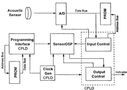
The system was designed to provide a simple user-friendly interface to the SensorDSP chip. There are three main components to the design: the programming interface, the analog input interface, and the heartbeat indicator. Other supporting components are the clock generation and power measurement circuits. The digital logic for the system is implemented in complex programmable logic devices (CPLD) [8]. A block diagram of the system is shown in Figure 3-1.
Acoustic Data Bus
Sensor c:
0.
Programming
Interface SensorDSP Input Control
CPLD)
oClock
+IN G n , Output Indicator
D. CPLDControl
---CPLD Figure 3-1: System Block Diagram
3.1
Programming Interface
The programming interface provides the distributed arithmetic tables for the linear filter, the instruction memory for the NLSL filter, the instruction memory for the micro-controller, and configuration/control codes. The programming interface con-sists of a 64Kx8 programmable read-only memory (PROM) [9], a parallel to serial shift register, and a finite state machine (FSM) controller.
3.1.1
JTAG Interface
Formally known as IEEE/ANSI standard 1149.1-1990, JTAG is a set of rules for-mulated by the Joint Test Action Group (JTAG). When applied at the chip level the standard helps reduce the cost of designing, testing and producing integrated circuits [10]. The JTAG standard makes use of a serial Test Access Port (TAP) to supply and extract information from an integrated circuit (IC). This information is used to program, test, and verify the operation of a given IC. In the application of the SensorDSP chip, the TAP is used to supply the chip with distributed arithmetic table entries for the linear filter, instructions for the non-linear/short-linear filter, in-structions for the micro-controller, and miscellaneous configuration words. Due to the variety of the information that needs to be provided to the chip, the JTAG standard
allows for a simple interface that requires a minimal number of external pins.
The TAP consists of a boundary/scan register and a finite state machine (FSM) controller. The state transition diagram of the FSM is shown in Figure 3-2. A test mode select (TMS) signal causes the TAP FSM to transition from state to state. The boundary/scan register is a shift register that receives its serial input from the "test data input" (TDI) signal. The output of the boundary/scan register is the "test data output" (TDO) signal. The clock signal to the FSM and register is called "test clock" (TCK). A TAP controller has an optional "test reset" (TRST) signal that restores the FSM to the "RUN-TEST/IDLE" state. The FSM changes state on the rising edge of TCK. The control signals TMS and TDI are required to be stable during the
0
0 Run Test Idle
1 1 Select-DR-Scan 0 Capture-DR 0 Shift-DR 0 10 Exit1-DR 0 Pause-DR 0 0 Exit2-DR Update-DR ______________1 1
Test Logic Reset
Select-IR-Scan Capture-IR 0 Shift-IR Exit1-IR 10 Pause-IR 0 01 Exit2-IR 1 Update-IR 0
Figure 3-2: JTAG TAP State Diagram
t0
circuitry, it is mandated by the JTAG standard that TMS and TDI only change on the falling edge of TCK.
The operation of the TAP controller is separated into two major functions for the purposes of this project: "Instruction Register Scan" (IR-Scan) and "Data Register Scan" (DR-Scan). While TMS is low, the TAP controller remains in the "Run-Test/Idle" state. When in the "Run-"Run-Test/Idle" state, the TAP controller will enter the "IR-Scan" state when TMS is held high for two rising edges of TCK followed by TMS being held low for two rising edges of TCK. An instruction can then be serially input to the chip. At the time when the last bit is clocked into the scan-register, TMS is brought high for two rising edges of TCK. This updates the instruction into the instruction register and returns the controller to the "Run-Test/Idle" state. In order to enter data into the data register, TMS is held high for one rising edge of TCK and then brought low. When the last bit is being input to the chip, TMS is brought high for two rising edges of TCK.
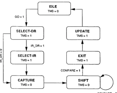
The TAP controller embedded in the SensorDSP chip meets the standards set by the IEEE 1149.1-1990 document [10]. In order to properly program the SensorDSP chip, a similar FSM controller was needed to generate the proper timing for the TMS signal. Figure 3-3 shows the state transition diagram of this FSM.
When the "IRJDR" signal is high, the FSM programs the instruction register. When "IRJDR" is low, the data register is programmed. The FSM outputs a "shift" signal when data is being shifted into the chip. It also outputs a "done" signal when it has finished shifting. These signals are passed to the program control FSM, which will be described in the next section.
3.1.2
Programming Interface Description
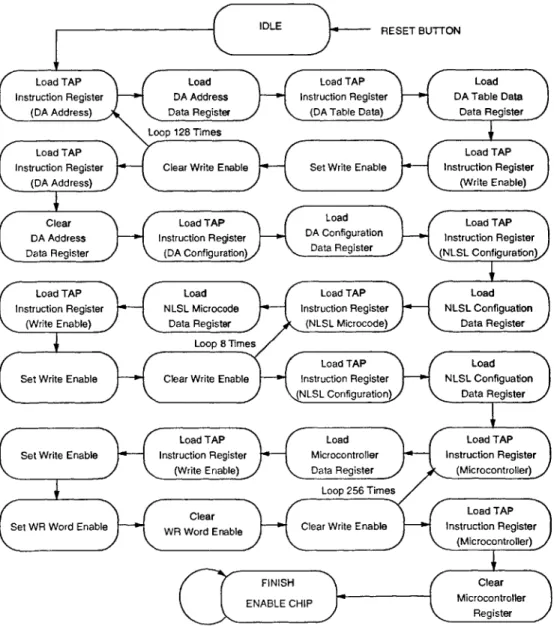
The FSM described in the previous section provides the necessary timing of the TMS signal. Since the bit-width of the serial input varies from 1 bit to 37 bits, the program control FSM is needed to keep track of which type of data is being programmed at any given time. A state transition diagram of the FSM is shown in Figure 3-4.
IDLE TMS =0 GO = 1 SELECT-DR UPDATE TMS=1 TMS=1 IRDR= 1 SELECT-IR EXIT TMS = I TMS = 1 COMPARE = I CA PTURE SHIFT TMS =0 TMS=0 COMPARE=0
Figure 3-3: JTAG Controller State Diagram
are summarized in Table 3.1. Each instruction is a 7-bit word. Each type of TAP instruction specified in Table 3.1 has an associated width. A list of these bit-widths is found in Table 3.2.
When loading distributed arithmetic table values, the first step is to supply the
DAINSTR1 instruction to the chip. Then the address that specifies a particular DA table entry is supplied to the data register of the TAP controller. Recall from
Chapter 2 that there are 16 distributed arithmetic tables and each table has 8 en-tries. The addressing scheme uses "one-hot encoding" for the 16 most significant bits
Mnemonic Binary Value Description
MUCTRL-INSTRO 0000001 Sets TAP to accept micro-controller instructions
NLSLJNSTRO 0000010 Sets TAP to accept NLSL instructions
NLSLINSTR1 0000100 Sets TAP to accept NLSL configuration settings
DA-INSTRO 0001000 Sets TAP to accept write enable bit for all units
DAINSTR1 0010000 Sets TAP to accept DA table addresses
DAINSTR2 0100000 Sets TAP to accept DA table values
DA_INSTR3 1000000 Sets TAP to accept DA configuration settings Table 3.1: TAP Instruction Words
C IDLED RESET BUTTON
Load TAP Load Load TAP Load
Instruction Register DA Address Instruction Register DA Table Data (DA Address) Data Register (DA Table Data) Data Register
Loop 128 Times
Load TAP Load TAP
Instruction Register Clear Write Enable Set Write Enable Instruction Register
(DA Address) (Write Enable)
Clear Load TAP Load Load TAPI
DA Address Instruction Register DA Configuration Instruction Register Data Register (DA Configuration) Data Register (NLSL Configuration)
Load TAP Load Load TAP Load
Instruction Register NLSL Microcode Instruction Register NLSL Configuation (Write Enable) Data Register (NLSL Microcode) Data Register
Loop 8 Times
Load TAP Load
Set Write Enable Clear Write Enable Instruction Register NLSL Configuation (NLSL Configuration' Data Register
Load TAP Load Load TAP
Set Write Enable Instruction Register Microcontroller Instruction Register (Write Enable) Data Register (Microcontroller)
Loop 256 Times
Clear Load TAP
Set WR Word Enable WR Word Enable Clear Write Enable Instruction Register (Microcontroller)
FINISH Clear
ENABLE CHIP Microcontroller Register
Instruction Type Bit-width TAP Instruction 7
Micro-controller Instruction 31
Micro-controller Write Enable 2
NLSL Filter Instruction 37 NLSL Configuration 9 NLSL WArite Enable 1 DA Table Address 19 DA Table Value 11 DA Table Write Enable 1
Table 3.2: Program Instruction Bit-sizes
(MSBs) of the address to select one of the 16 tables. The 3 least significant bits (LSBs) represent the binary number of which table entry is selected. After each table value is loaded into the boundary scan register, the write enable is toggled. Toggling the write enable is accomplished in the same manner as loading addresses or data into the scan register. The process of loading table addresses and table data values is repeated 128 times since there are 8 table entries in 16 tables. After all tables have been programmed, the DA address register must be cleared. Clearing the address register allows data from the input shift register to access the DA tables instead of the scan register.
After programming the DA table values, the DA configuation register must be programmed. The DA table configuration setting is a 34 bit word. The 16 MSBs are enable bits for each DA table. The next 3 bits select the input data bit-width. The next 4 bits are the truncation setting for the linear filter accumulator. The binary values for the bit-width and truncation settings are given in Table 3.3. The remaining
11 bits are the initial condition of the linear filter. The instruction format of the DA
table programming words is shown in Figure 3-5.
Once the programming for the DA unit is complete, the NLSL instructions must be programmed. This process is begun by initializing the NLSL configuration regis-ter. Then the 8 NLSL instructions can be programmed. The final step is to set the configuration register to the appropriate truncations settings for the SAC and MAC
Truncation Settings Binary Truncation 0001 Output = bits[11:0] 0010 Output = bits[15:4] 0100 Output = bits[19:8] 1000 Output = bits[23:12] Bit-width Settings Binary Bit-width 001 1 010 2 100 4 000 8
Table 3.3: Truncation and Bit-width Configuration Settings
accumulators. The binary encoding of the truncation setting is identical to the DA truncation settings shown in Table 3.3. The NLSL instruction format can also be seen in Figure 3-5. The first 3 MSBs are the instruction address. The next 7 bits are the Square/Accumulate instruction. The next 11 bits are the Multiply/Accumulate instruction. The remaining 16 bits are the Load/Store instruction. The NLSL con-figuration word is 9 bits wide. The MSB is the the filter enable. The next 4 bits are the truncation setting for the SAC (ACCO). The remaining 4 bits are the truncation setting for the MAC (ACC1).
The last remaining sets of information to be programmed into the chip are the micro-controller instructions. The micro-controller programming word is 31 bits wide. The MSB is an enable bit and should always be set to 1. The next 8 MSBs are the address of the instruction to be entered. An empty (zero) bit is placed after the address. The remaining 21 bits are the controller instruction. The micro-controller instruction memory load is repeated for each of the 256 instructions that can be loaded into the SensorDSP chip.
All of the programming data is stored in a 64Kx8 bit programmable read-only
memory (PROM). Each byte is loaded from the PROM into a shift register and shifted (LSB first) into the SensorDSP chip through the TDI pin. Since the programming
18 3 2 0
Table Select 16 bit (one-hot) Entry Addr
DA TABLE ADDRESS
10 0
DA Table Value
DA TABLE VALUE
33 18 17 15 14 11 10 0
DA Table Enable (one-hot encoded) Bitwidth Truncation DA Table Initial Condition
DA TABLE CONFIGURATION
36 34 33 27 26 16 15 0
Address Square/Acc Instr. Multiply/Acc Instruction Load/Store Unit Instruction
NLSL INSTRUCTION & ADDRESS
8 7 4 3 0
En Truncation Truncation En ACCI ACCO
NLSL CONFIGURATION
31 30 22 21 20 0
En Instruction Address 0 Microcontroller Instruction (21 bits) MICROCONTROLLER INSTRUCTION & ADDRESS
Figure 3-5: Programming Instruction Formats
FSM is responsible for controlling the TMS signal, the load signal and the shift signal
to the shift register. The programming controller maintains a count of how many bits have been shifted, a count of how many times a particular sequence has been repeated, and the current address for the PROM. A block diagram of the programming controller is shown in Figure 3-6. For words longer than 8 bits, the word must be contained in multiple addresses of the PROM. For words less than 8 bits, the remaining bits of the PROM address are left unused.
The parallel to serial shift register and address counters for the PROM, as well as, the finite state machine are implemented in a single complex programmable logic device (CPLD).
"Repeat Counter" 8 bit Counter 8 -1 z wL "Shift Counter" 5 bit Counter < -J C) z 5 ENABLE 3 bit , Counter CLEAR ENABLE w -J z 12
12 bit Address Counter 8 bit Shift Register
Figure 3-6: Programming Interface Block Diagram
3.2
Analog Sensor Interface
The analog acoustic sensor is a microphone and amplifier contained in a small package that can be placed against the neck or chest of an individual to sense and amplify. The sensor was provided my the Army Research Laboratory. The amplifier has 4 gain settings (20, 10, 3, 1). The output of the analog sensor is sampled with an 8 bit analog to digital converter (A/D). The A/D converter is an Analog Devices AD670 successive approximation converter [11]. The AD670 was chosen because it has the capability to operate in a bipolar or unipolar analog input. It has an adjustable
I
Cc q: wU FSM Controller ROM C') a: I- LOADin bipolar mode with an analog input range of +1.28V to -1.28V. The output format is set to be 2's complement.
One potential problem with the analog interface is the conversion time of the A/D. The AD670 has a maximum conversion time of 10ps. During conversion, the status bit of the A/D is a logic high. For the intended application, the sample rate is less than 1kHz, therefore the conversion time is not a limiting factor.
Since the SensorDSP chip expects a serial input data stream, the parallel output of the AD670 must be converted to serial. This is done with a shift register within a CPLD similar to the programming interface. A strobe from the I/O controller is sent to the A/D initiating a conversion. The data is then loaded into the shift register. During the next N clock cycles (where N is the desired bit-width of the input data) data is shifted (MSB first) into the SensorDSP chip. At the end of N clock cycles the A/D receives another strobe and begins conversion again. A timing diagram of the A/D interface is shown in Figure 3-7.
CLK
R/W A/D DATA
SHIFT REG SHIFTXSHIFTXSHIFTXSHIFTXSHIFTXLOAD SHIFT
Figure 3-7: A/D Converter Timing
A significant part of properly using the system is choosing an appropriate matched
filter for the desired application. As such it is useful to have a controlled input data stream to the chip, for testing and verification purposes. The SensorDSP system provides the capability to insert a PROM containing test data that can be supplied to the chip instead of data from the A/D converter. This is done by placing the
PROM's data lines on the bus with the A/D data. The I/O controller deactivates (sets the outputs to tri-state) either the A/D or the PROM based on a selection switch on the board. The I/O controller increments the PROM address at the same rate it triggers the A/D, thus simulating the presence of real data. A block diagram of the Analog Sensor Interface is shown in Figure 3-8.
8 Data Bus 8
Analog ASerial Out
, AD67 PROMSHIFT
Input r e/CE n aREG
R/W /CE
INPUT LOD CONTROL
SHIFl
Bit-Width Select
Figure 3-8: Analog Sensor Interface Block Diagram
3.3
Heartbeat Indicator
The SensorDSP chip has a limited output capability. Due to constraints on the number of pins, the chip only has a 12-bit output bus. To increase functionality and testability, this bus is 8-way multiplexed via a 3-bit select input. The data available from this bus are listed in Table 3.4.
The 3-bit selection input is supplied from the output controller. The output controller is contained within a complex programmable logic device (CPLD). The
Table 3.4: SensorDSP Output Bus Selection
is to watch the program counter. The assembly code that implements the heartbeat detection algorithm is written such that the program jumps to a unique location of the instruction memory when a heartbeat is detected. By default, the output controller sets the SensorDSP output bus multiplexer to the program counter.
Eight external switches on the system board allow the user to enter which in-struction memory address the controller will watch for. When the program counter matches the value on the input switches, an indicator light emitting diode (LED) is lit. The LED is held lit for a fixed amount of time to ensure that it is visible to the human eye. In addition to a single LED indicator, three hexadecimal numeric displays are available to display information extracted from the SensorDSP chip. For the given application, the hex displays provide an approximate "beats per minute" value. A block diagram of the heartbeat indicator circuit is shown in Figure 3-9.
The output controller CPLD can easily be reprogrammed to extract other useful information from the chip such as filtering results or micro-controller calculations.
3.4
Clock Generation
As mentioned in Chapter 1, the SensorDSP chip operates on a slow clock and a fast clock. The SensorDSP has an embedded clock generation module. This module takes in a clock reference ( rei) that is twice the desired fast clock frequency. Based on the value of the clock configuration bits (CCONF switches), the (ref clock is divided by a
Binary Select Test Bus Output
000 DA Filter Output 001 NLSL AccO (SAC) 010 NLSL Acci (MAC)
011 DA Filter Buffer Output 100 NLSL Acc0 (SAC) Buffer Output
101 NLSL Acci (MAC) Buffer Output 110 Micro-controller Memory Data Bus 111 Micro-controller Program Counter
HEXADECIMAL DISPLAY E lj SELECT LED "3\ / SENSOR DSP OUTPUT CHIP CONTROL TEST PORT 8 CONTROL SWITCHES
Figure 3-9: Heartbeat Indicator Block Diagram
scaling factor to produce the slow clock. Equation 3.1 calculates the clock frequency based on the frequency of the (ref signal and the value of the CCONF switches. The value of (1),ef for the system is 230.4 kHz.
fslowelk = 2C+2 (3.1)
The clock generation module outputs the desired clock as well as the read trigger signal (RD-TRIG). The RD-TRIG signal is a clock that has a 45 degree phase shift with reference to the system clock. This signal is used for the timing of memory
accesses within the chip. Figure 3-10 shows the timing of this signal.
CLK RD TRIG
Figure 3-10: Read Trigger Timing
It was the designer's choice to isolate the clock generator module from the chip architecture. Subsequently, the "CLK" and "RDTRIG" signals must be externally fed back into the chip. As such, the user can opt to use the internal clock generator module or the external clock generator module. Since there is combinational logic that enables the chip to switch clock frequencies there is a potential for glitches or "runt pulses" to appear on the clock signal that could cause the system to execute an incorrect instruction or skip an instruction. Because of the overall low speed operation of the system, the potential for this error is small. Additional precautions have been taken to avoid this problem by adding NOP instructions in the microcode at the locations where this glitch could occur. This is easy to do since the switching is controlled by a microcode instruction. For almost all applications, using the internal clock module is recommended.
In addition to generating the clock for the SensorDSP chip, the external clock module generates the clock for all other components in the system. The input/output controller receives the same slow clock as does the SensorDSP chip. The programming controller receives a separate 14.4 kHz clock. Figure 3-11 depicts a block diagram of the clock generator subsystem.
C.i Z -LD-W-U CCONF 2XCLK CLK TCK T 0 SDSPCLK t ~ T 0 - RDTRIG FAST MODE
Figure 3-11: Clock Generation Circuitry
3.5
Power Measurement
The overall goal of the system is to demonstrate the functionality of the signal process-ing application at ultra low power levels. First, an ammeter connection is provided on the board to accurately measure the current being drawn from the power
sup-ply. Second, a bar-graph LED display in embedded in the system to allow for an
approximate power measurement. A schematic of the power measurement circuitry is shown in Figure 3-12. This circuit utilizes a bank of eight comparators and a resistor voltage divider network. A resistor is placed in series between VDD and the chip. The comparator array detects the voltage drop across the resistor and lights the appro-priate LEDs of the bar-graph. Since the current drawn by the chip is on the order of
lptW,
or less the resistance of the series resistor must be on the order of 200 kQ in order for there to be a noticeable voltage drop. Because of this voltage drop, the external VDD will need to be increased to maintain the necessary 1.5V delivered to the chip. The default setting for power measurement yields approximately 0.5PA perVdd +L 1 00k 200k 150k SensorDSP Chip LO) C,.j20 U20 LO) C," j1250
Figure 3-12: Power Measurement Schematic
Lea
0
3.6
Battery Vs. External Supply
The option to utilize battery power instead of an external power supply is provided in the system. The internal power supply generation is provided by a 9V battery and two voltage regulators. One is a fixed, 5V voltage regulator [14] that supplies power to all the support electronics on the board. The second is an adjustable voltage regulator [13] that supplies the VDD of the SensorDSP chip. The schematic for the internal supply is shown in Figure 3-13. Jumper wires on the board are placed by the user to select external or internal mode.
LM340 5V Fixed 5V Regulator lu T lu LM317 Adjustable : Vdd + Regulator 9V -_40 U lu 5k
Figure 3-13: Power Regulation Schematic
3.7
Test Ports
The SensorDSP board has 7 test ports that can be used to monitor the operation of the board. Table 3.5 lists all signals available from the test ports. Figure 3-14 shows the pin diagram of a standard test port. Each test port is a 16 pin dual-in-line header pin. Eight of the pins are signal pins; the remaining eight are connected to ground.
8 7 6 5 4 3 2 1
00000000
00000000
GROUND
TP#
Figure 3-14: Test Point Pin Diagram
TP# Pin
#'s
Signal Name1 1 - 8 Program PROM Data Bus
2 1 - 8 Program PROM Address Bus (7:0)
3 1 SensorDSP TDI
3 2 SensorDSP TMS
3 3 SensorDSP TRST
3 4 Program IDLE
3 5 - 8 Program PROM Address Bus (11:8)
4 1 - 8 SensorDSP Test Port (11:4)
5 1 - 4 SensorDSP Test Port (3:0)
5 5 PRE
5 6 WORD-EN
5 7 DLATCH
5 8 BUFWEN
6 1 - 8 Test Data PROM Data Bus
7 1 FASTMODE 7 2 XOUT 7 3 SensorDSP TDO 7 4 RD-TRIG 7 5 CLKIN 7 6 LED-DETECT 7 7 SensorDSP TCK 7 8 XIN
Table 3.5: Test Port Signals
Chapter 4
System Details
"Using The SensorDSP System"
This chapter contains instructions for using the SensorDSP system. The following is a list of required components in order to properly use the system.
1. The SensorDSP board
2. The Heart Sensor Amplifier and Filter or compatible analog signal receiver
3. Dual Source Adjustable Power Supply
4. Cypress Warp2ISR Programmable Logic Kit for PC (VHDL or Verilog) Flash370i Series
5. The SensorDSP Initialization Program (for Unix)
6. A Programmable Read-Only Memory Programmer (compatible with Intel MCS-86 Hexadecimal Format)
There are many steps that must be followed in order to successfully program and use the SensorDSP system. This chapter is a step-by-step "walk-through" of the usage of the system. The topics that are covered in this chapter are:
o Compiling Program Data
o Running the system
o Using the test data input
o Extracting data from the board
o Additional Features
o Troubleshooting
Figure 4-1 is a floor-plan of the system board. All parts, switches, ports, and displays can easily be identified by referring to Figure 4-1 and Table 4.1, which lists the parts of the board with brief descriptions.
4.1
Compiling Program Data
The compilation of program data is accomplished by running the "SensorDSP Ini-tialization Program". The program enables the user to enter linear filter coefficients,
NLSL instructions, and micro-controller instructions. The program then generates
an Intel MCS-86 hexadecimal formatted file (filename.ntl). The PROM can then be programmed and inserted into the system board. Before running the "SensorDSP Initialization Program" there are several steps that must be performed.
1. Choose coefficients of the matched filter. The filter coefficients should be
ar-ranged in a text file with a carriage return separating each number. There should be a maximum of 64 coefficients and each coefficient must be in the
A
R6-Pot
J6 5J71
Power Jumpers RED
D30
00
Ammeter Ammeter Out In51
Ammeter Jumper TF GREEN OD1 Power Jumpers 4 | CONTROL SWITCHES D20
HEART DETECT LED Hexadecimal Display TP6 SensorDSP PGM CTRL I/O CTRL TP5 IT P=7 -H PGMROMSEL CCONF CLKGEN CLK Jumpers DATAROMSEL S3 S4 S5 S8 S10 S9 RESET STARY7
0 TWINAX Global Enable Unused Input/Output Control Reset U ModeUP: Test Data DN: Sensor Data
nused
Figure 4-1: SensorDSP System Board Floor-plan
9V BATTERY PGM PROM TEST DATA PROM

![Figure 1-4: Distributed Arithmetic ROM and Accumulator Structure [1, p. 119]](https://thumb-eu.123doks.com/thumbv2/123doknet/14675161.557788/19.918.222.816.194.683/figure-distributed-arithmetic-rom-accumulator-structure-p.webp)
![Figure 2-2: Signal Processing Chip Architecture [1, p. 128]](https://thumb-eu.123doks.com/thumbv2/123doknet/14675161.557788/24.918.139.755.471.653/figure-signal-processing-chip-architecture-p.webp)
![Figure 2-3: Linear Filter Implementation Architecture [1, p. 130]](https://thumb-eu.123doks.com/thumbv2/123doknet/14675161.557788/25.918.192.740.137.562/figure-linear-filter-implementation-architecture-p.webp)
![Figure 2-4: DA Unit Shift Register Implementation [1, p. 131]](https://thumb-eu.123doks.com/thumbv2/123doknet/14675161.557788/26.918.137.770.381.880/figure-da-unit-shift-register-implementation-p.webp)
![Figure 2-5: NLSL Filter Implementation Architecture [1, p. 131]](https://thumb-eu.123doks.com/thumbv2/123doknet/14675161.557788/28.918.188.709.125.458/figure-nlsl-filter-implementation-architecture-p.webp)