HAL Id: hal-00387395
https://hal.archives-ouvertes.fr/hal-00387395
Preprint submitted on 25 May 2009
HAL is a multi-disciplinary open access
archive for the deposit and dissemination of
sci-entific research documents, whether they are
pub-lished or not. The documents may come from
L’archive ouverte pluridisciplinaire HAL, est
destinée au dépôt et à la diffusion de documents
scientifiques de niveau recherche, publiés ou non,
émanant des établissements d’enseignement et de
Hyperbolic conservation laws on the sphere. A
geometry-compatible finite volume scheme
Matania Ben-Artzi, Joseph Falcovitz, Philippe G. Lefloch
To cite this version:
Matania Ben-Artzi, Joseph Falcovitz, Philippe G. Lefloch. Hyperbolic conservation laws on the sphere.
A geometry-compatible finite volume scheme. 2009. �hal-00387395�
Hyperbolic conservation laws on the sphere.
A geometry-compatible finite volume scheme
Matania Ben-Artzi, Joseph Falcovitz,
Institute of Mathematics, Hebrew University, Jerusalem 91904, Israel.
E-mail: [email protected], [email protected]
Philippe G. LeFloch
Laboratoire Jacques-Louis Lions,
Centre National de la Recherche Scientifique (CNRS), Universit´e Pierre et Marie Curie (Paris 6), 4 place Jussieu,
75252 Paris, France. E-mail: [email protected]
Abstract
We consider entropy solutions to the initial value problem associated with scalar nonlinear hyperbolic conservation laws posed on the two-dimensional sphere. We propose a finite volume scheme which relies on a web-like mesh made of segments of longitude and latitude lines. The structure of the mesh allows for a discrete version of a natural geometric compatibility condition, which arose earlier in the well-posedness theory established by Ben-Artzi and LeFloch. We study here several classes of flux vectors which define the conservation law under consideration. They are based on prescribing a suitable vector field in the Euclidean three-dimensional space and then suitably projecting it on the sphere’s tangent plane; even when the flux vector in the ambient space is constant, the corresponding flux vector is a non-trivial vector field on the sphere. In particular, we construct here “equatorial periodic solutions”, analogous to one-dimensional periodic solutions to one-one-dimensional conservation laws, as well as a wide variety of stationary (steady state) solutions. We also construct “confined solutions”, which are time-dependent solutions supported in an arbitrarily specified subdomain of the sphere. Finally, representative numerical examples and test-cases are presented.
Key words: hyperbolic conservation law, sphere, entropy solution, finite volume scheme, geometry-compatible flux.
Contents
1 Introduction 2
2 Families of geometry-compatible flux vectors 5 3 Special solutions of interest 7 3.1 Periodic equatorial solutions 7
3.2 Steady states 8
3.3 Confined solutions 9
4 Design of the scheme 10
4.1 Computational grid 10
4.2 Geometry-compatible discretization of the divergence operator 10 4.3 Godunov-type approach to the numerical flux 12 4.4 Solution to the Riemann problem 14
4.5 Convergence proof 15
5 Second-order extension based on the GRP solver 16
6 Numerical tests 18
6.1 First test case: equatorial periodic solutions 18 6.2 Second test case: steady state solutions 19 6.3 Third test case: confined solutions 20
References 22
1. Introduction
In this paper, building on our earlier analysis in [6,2] we study in detail the class of scalar hyperbolic conservation laws posed on the two-dimensional unit sphere
S2=!(x, y, z) ∈ R3, x2+ y2+ z2= 1".
We propose a Godunov-type finite volume scheme that satisfies certain important con-sistency and convergence properties. We then present a second-order extension based on the generalized Riemann problem (GRP) methodology [3].
It should be stated at the outset that an important motivation for this paper is the need to provide accurate numerical tools for the so-called shallow water system on the sphere. This system is widely used in geophysics as a model for global air flows on the rotating Earth [7]. In its mathematical classification it is a system of nonlinear hyperbolic PDE’s posed on the sphere. Its physical nature dictates that it can be described “invariantly”, namely in a way which is independent of any particular coordinate system. Locally, it has the (mathematical) character of a two-dimensional isentropic compressible flow, whereas globally the spherical geometry plays a crucial role in shaping the nature of solutions –which, as expected for nonlinear hyperbolic equations, may contain propagating discon-tinuities such as shock fronts or contact curves. Thus, the relation of the present study to the shallow water system is analogous to the connection between Burgers’ equation and the system of compressible fluid flow (say, in the plane). In fact, in light of this analogy it is somewhat surprising that in the existing literature so far, virtually all treatments, theoretical as well as numerical, were confined to the Cartesian setting. In particular, to the best of our knowledge, there have been no systematic numerical studies of scalar conservation laws on the sphere.
Having introduced the scalar conservation law as a simple model for more complex physical systems, we should emphasize here also the intrinsic mathematical interest of
the model under consideration. It is already known (see [5] and references there) that even in the Cartesian setting, the two-dimensional scalar conservation law displays a wealth of wave interactions typical of the physical phenomena (such as triple points, sonic shocks, interplay of rarefactions and shocks coming from different directions and more). As we show here, “geometric effects”, superposed on the (necessarily) two-dimensional frame-work, carry the scalar model still further. For example, the concept of “self-similar” solu-tions makes no sense here. In particular, one loses the Riemann solusolu-tions, a fundamental building block in many schemes (of the so-called “Godunov-type”). On the other hand, it allows for large classes of non-trivial steady states, periodic solutions, and solutions supported in specified subdomains. All these have natural consequences in developing numerical schemes; they offer us a variety of test-cases amenable to detailed analysis, to be compared with the computational results.
In practical applications a finite volume scheme requires a specification of a coordinate system, where the symmetry-preserving latitude–longitude coordinates are the “natural coordinates” of preferred choice. The proposed finite volume scheme in this paper is based on these natural coordinates, but should pay attention to the artificial singularities at the poles.
In [2], a general convergence theorem was proved for a class of finite volume schemes for the computation of entropy solutions to conservation laws posed on a manifold. As a particular example, the case of the sphere S2was discussed, both from the points of view
of an “invariant” formalism and that of an “embedded” coordinate-dependent formula-tion. In the present study we focus on the sphere S2and we actually construct, in a fully
explicit and implementable way, a finite volume scheme which is geometrically natural and can be viewed as an extension of the basic Godunov scheme for one-dimensional conservation laws. Furthermore, we prove that our scheme fulfills all of the assumptions required in [2], which ensures its strong convergence toward the unique entropy solution to the initial value problem under consideration. We then describe the GRP extension of the scheme, whose convergence proof is still a challenging open problem.
The theoretical background about the well-posedness theory for hyperbolic conserva-tion laws on manifolds was established recently by Ben-Artzi and LeFloch [6] together with collaborators [1,2,8,9]. An important condition arising in the theory is the “zero-divergence” or geometric-compatibility property of the flux vector; a basic requirement in our construction of a finite volume scheme is to formulate and ensure a suitable discrete version of this condition.
We conclude this introduction with some notation and remarks connecting the present paper to the general finite volume framework presented in [2]. Following the terminology therein, we use an “embedded” approach to the spherical geometry, namely, we view the sphere as embedded in the three-dimensional Euclidean space R3. We denote by x
a variable point on the sphere S2, which can be represented in terms of its longitude λ
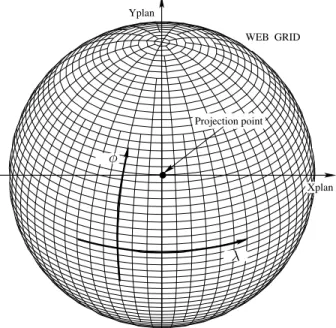
and its latitude φ. Following the conventional notation in the geophysical literature we assume that
0 ≤ λ ≤ 2π, −π2 ≤φ≤ π 2, so that the “North pole” (resp. “South pole”) is at φ = π
2 (resp. −φ = π
2) and the
equator is!φ = 0, 0 ≤ λ ≤ 2π". (See Figure 1.) The coordinates inR3 are denoted by
(x1, x2, x3) ∈ R3 and the corresponding unit vectors are i1, i2, i3. Thus, at each point
iλ= − sin λ i1+ cos λ i2,
iφ= − sin φ cos λ i1− sin φ sin λ i2+ cos φ i3.
It should be observed that while a choice of a coordinate system is necessary in practice, it always introduces singularities and the unit vectors given above are not well-defined at the poles and, therefore, in the neighborhood of these points it cannot be used for a representation of smooth vector fields (such as the flux vectors of our conservation laws). We also emphasize that the status of these two poles is equivalent to the one of any other pair of opposite points on the sphere. When such local coordinates are introduced, special care is needed to handle these points in practice, and this is precisely why we advocate a different approach.
Continuing with the description of our “embedded” approach, we define the unit nor-mal nx, to S2 at some point x by
nx= cos φ cos λ i1+ cos φ sin λ i2+ sin φ i3.
Then, any tangent vector field F to S2 is represented by
F = Fλiλ+ Fφiφ
and the tangential gradient operator is ∇T = # 1 cos φ ∂ ∂λ, ∂ ∂φ $ .
Thus, the (tangential) gradient of a scalar function h(λ, φ) is given by ∇Th = 1 cos φ ∂h ∂λiλ+ ∂h ∂φiφ, (1.1)
and the divergence of a vector field F is ∇T · F = 1 cos φ # ∂ ∂φ(Fφ cos φ) + ∂ ∂λFλ $ . (1.2)
Given now a vector field F = F(x, u) depending on a real parameter u, the associated hyperbolic conservation law under consideration is
∂u ∂t + ∇T ·
%
F(x, u)&= 0, (x, t) ∈ S2
× [0, ∞), (1.3) where u = u(x, t) is a scalar unknown function, subject to the initial condition
u(x, 0) = u0(x), x ∈ S2 (1.4)
for some prescribed data u0 on the sphere. As mentioned above, we will impose on the
vector field F(x, u) an additional “geometry compatibility” condition.
An outline of this paper is as follows. In Section 2, we consider the construction of geometry-compatible flux vectors, while Section 3 is devoted to a description of several families of special solutions associated with the constructed flux vectors. In Section 4 we discuss our (first-order) finite volume scheme, which can be regarded as a Godunov-type scheme. We prove that it satisfies all of the assumptions imposed on general finite volume schemes in [2], and we conclude that it converges to the exact (entropy) solution. In Section 5 we describe the (second-order) GRP extension of the scheme. Finally, in Section 6 we present a variety of numerical test cases.
WEB GRID Xplan Yplan Projection point λ φ
Fig. 1. Web grid on a sphere
2. Families of geometry-compatible flux vectors
As pointed out in [2], every smooth vector field F(x, u) on S2 can be represented in
the form
F(x, u) = n(x) × Φ(x, u), (2.1) where Φ(x, u) is a restriction to S2of a vector field (in R3) defined in some neighborhood
(i.e., a “spherical shell”) of S2and for all values of the parameter u. The basic requirement
imposed now on the flux vector F(x, u) is the following divergence free or geometric compatibility condition: For any fixed value of the parameter v∈ R,
∇T· F(x, v) = 0. (2.2)
A flux vector F(x, u) satisfying (2.2) is called a geometry-compatible flux [6]. Note that this condition is equivalent, in terms of the nonlinear conservation law (1.3), to the following requirement: constant initial data are (trivial) solutions to the conservation law. In the case of the sphereS2the condition (2.2) can be recast in terms of a condition
on the vector field Φ(x, u) appearing in (2.1). See [2, Proposition 3.3].
Our main aim in the present section is singling out two (quite general) families of geometry-compatible fluxes of particular interest, which are amenable to detailed ana-lytical and numerical investigation.
The flux-vectors of interest are introduced by way of the following two claims.
Claim 2.1 (Homogeneous flux vectors.) If the three-dimensional flux Φ(x, u) = Φ(u) is independent of x (in a neighborhood of S2), then the corresponding flux vector F(x, u)
Proof. The following decomposition applies to any vector Φ(u)∈ R3 in the form
Φ(u) = f1(u) i1+ f2(u) i2+ f3(u) i3, (2.3)
so that F(x, u) = Fλ(λ, φ, u) iλ+ Fφ(λ, φ, u) iφ, with
Fλ(λ, φ, u) = f1(u) sin φ cos λ + f2(u) sin φ sin λ − f3(u) cos φ,
Fφ(λ, φ, u) = −f1(u) sin λ + f2(u) cos λ.
(2.4) We can directly apply the divergence operator (1.2) to F(x, u) and the desired claim follows. !
Claim 2.2 (Gradient flux vectors.) Let h = h(x, u) be a smooth function of the variables x (in a neighborhood of S2) and u ∈ R, and consider the associated
three-dimensional flux Φ(x, u) = ∇h(x, u) (restricted to x ∈ S2). Then, the flux vector F(x, u)
given by (2.1) is geometry-compatible.
Proof. We use the divergence theorem in an arbitrary domain D ⊆ S2 with smooth
boundary ∂D: ' D∇ T · (F(x, v)) dσ = ' ∂DF(x, v) · ν(x) ds =' ∂D ( n(x) × ∇h(x, v))· ν(x) ds,
where ν(x) is the unit normal (at x) along ∂D ⊂ S2, dσ is the surface measure on S2,
and ds is the arc length along ∂D.
In particular, n(x) × ν(x) = t(x) coincides with the (unit) tangent vector to ∂D at x. It follows that the triple product(n(x) × ∇h(x, u))· ν(x) = ∇h(x, u) · t(x) is nothing but the directional derivative ∇∂D of h along ∂D. Since
' ∂D∇ ∂Dh ds = 0, we thus find ' D∇ T· F(x, u) dσ = 0,
and since this holds for any smooth domain D, we conclude that ∇T · F(x, v) = 0 for all
v∈ R. !
Remark 2.3 1. Claim 2.1 is a special case of Claim 2.2. Indeed, by taking in the latter h(x, u) = x1f1(u) + x2f2(u) + x3f3(u) we obtain the conclusion of the former. However,
we chose to single out Claim 2.1 as a special case since it will serve in obtaining special solutions (Section 3) and in dealing with numerical examples (Section 6).
2. The steps in the construction of the gradient flux vector in Claim 2.2 are “linear in nature”, namely if h(x, u) = h1(x, u) + h2(x, u) then the corresponding
(geometry-compatible) flux vectors satisfy F(x, u) = F1(x, u)+F2(x, u). However, it is clear that the
corresponding solutions to (1.3) do not add up linearly, due to the nonlinear dependence in u.
3. Special solutions of interest 3.1. Periodic equatorial solutions
The scalar conservation laws discussed in this paper have two basic features: – The problem is necessarily two-dimensional (in spatial coordinates).
– The geometry plays a significant role, inasmuch as the flux vectors are subject to geometric constraints.
It should be noted that even within the framework of Euclidean two dimensional con-servation laws there is a great wealth of special solutions, displaying complex wave in-teractions, such as triple points, sonic shocks and more. We refer to [10,5] for detailed treatments of the theoretical and numerical aspects.
In the situation under consideration in the present paper, geometric effects yield a large variety of non-trivial steady states, solutions supported in arbitrary subdomains, etc. In this section we consider such solutions by selecting some special flux vectors F(x, u) on S2. This is accomplished by making special choices of Φ(x, u) in the general
representation (see (2.1)) F(x, u) = n(x) × Φ(x, u), where Φ(x, u) is a restriction to S2
of a vector field (in R3) defined in some neighborhood (i.e., “spherical shell”) of S2 and
for all values of the parameter u.
We begin our discussion with the case of periodic equatorial solutions, defined as follows. Taking f1(u) = f2(u) ≡ 0 in the general decomposition (2.3) so that, by (2.4),
Fλ(λ, φ, u) = −f3(u) cos φ,
Fφ(λ, φ, u) = 0,
the conservation law (1.3) takes the particularly simple form ∂u ∂t − ∂ ∂λf3(u) = 0, (x, t) ∈ S 2 × [0, ∞). (3.1) In particular, obtain the following important conclusion.
Corollary 3.1 (Solutions with one-dimensional structure.) Let *u = *u(λ, t) be a solution to the following one-dimensional conservation law with periodic boundary con-dition
∂u* ∂t −
∂
∂λf3(*u) = 0, 0 < λ ≤ 2π, *u(0, t) = *u(2π, t),
and let +u = +u(φ) be an arbitrary function. Then, the function u(λ, φ, t) = *u(λ, t) +u(φ) is a solution to the conservation law (3.1).
It follows that all periodic solutions from the one-dimensional case can be recovered here as special cases. However, in numerical experiments the computational grid is two-dimensional, so it is not obvious that the accuracy achieved in the computation of the former can indeed be achieved in the numerical scheme implemented on the sphere. This issue will be further discussed below, in Section 6.
3.2. Steady states
Let F = F(x, u) be a flux vector and u0 : S2 → R be an initial function such that
∇T ·
(
F(x, u0(x)))≡ 0. Then, clearly u0is a stationary solution (or steady state) to the
conservation law. In fact, we can show that there exist many (analytically computable) non-trivial steady state solutions, as follows.
Claim 3.2 (A family of steady-state solutions.) Let h = h(x, u) be a smooth func-tion defined for all x in a neighborhood of S2, and consider the associated gradient flux
vector Φ = ∇h (as in Claim 2.2). Suppose the function u0: S2→ R satisfies the condition
∇yh(y, u0(x))|y=x= ∇xH(x), x ∈ S2, (3.2)
where H = H(x) be a smooth function defined in a neighborhood of S2. Then, u 0 is a
stationary solution to the conservation law (1.3).
Proof. We follow the proof of Claim 2.2 and the notation therein. Using the divergence theorem in an arbitrary domain D ⊆ S2 with smooth boundary ∂D, we obtain
' D∇ T· ( F(x, u0(x)))dσ = ' ∂D F(x, u0(x)) · ν ds =' ∂D ( n(x) × ∇xH(x))· ν(x) ds.
where, as before, ν(x) is the unit normal, dσ the surface measure, and ds the arc length. In particular, n(x) × ν(x) = t(x), the (unit) tangent vector to ∂D at x. It follows that the triple product (n(x) × ∇xH(x))· ν(x) = (∇xH(x))· t(x) is the directional derivative
of H along ∂D. Thus, '
D∇ T ·
(
F(x, u0(x)))dσ = 0,
and since this holds for any smooth domain D, it follows that ∇T ·
(F(x, u
0(x))) ≡ 0,
which concludes the proof. !
The above claim yields readily a large family of non-trivial stationary solutions, as expressed in the following corollary.
Corollary 3.3 Consider the flux vector F = F(x, u) given by F(x, u) = n(x) ×(f1(u) i1),
for an arbitrary choice of function f1= f1(u). Then, any function u0= u0(x1) depending
only on the first coordinate x1 is a stationary solution to the conservation law
(associ-ated with this flux). In particular, in polar coordinates (λ, φ) any function of the form u0(λ, φ) = g(cos φ cos λ) is a stationary solution.
Proof. According to Claim 2.1 this flux vector is associated with the scalar function h(x, u) = x1f1(u). So we can invoke Claim 3.2 with H(x) = H(x1) such that H!(x1) =
Remark 3.4 This corollary enables us to construct stationary solutions supported in “bands” on the sphere. This is accomplished by taking u0 = u0(x1) to be supported in
0 < α < x1< β < 1. Observe that this band is not parallel neither to the latitude curves
(φ = const) nor to the longitude curves (λ = const).
There is yet another possibility of obtaining stationary solutions, where all three coor-dinates are involved, as stated now. This example can also be derived from the previous one by applying a rotation in R3.
Corollary 3.5 Consider the flux vector F = F(x, u) be given by F(x, u) = n(x) × (f1(u) i1+ f2(u) i2+ f3(u) i3)
= f(u) n(x) × (i1+ i2+ i3),
in which all three components coincide: f1(u) = f2(u) = f3(u) = f(u). Then, any
func-tion of the form u0(x) = *u0(x1+ x2+ x3), where *u0 depends on one real variable, only,
is a stationary solution to the conservation law associated with the above flux.
Proof. Following the proof of the previous corollary, we now take H(x) = H0(x1+x2+x3),
where H!
0(ξ) = f(*u0(ξ)). !
Remark 3.6 In analogy with Remark 3.4, this result allows us to construct stationary solutions in a spherical “cap” (a piece of the sphere cut out by a plane). In Section 6 below, we will provide numerical test cases for such stationary solutions.
3.3. Confined solutions
If in the conservation law (1.3) we have F(x, u) ≡ 0 for x in the exterior of some domain D ⊆ S2, identically in u
∈ R, and if the initial function u0(x) vanishes outside
of D, then clearly the solutions satisfy u(x, t) = 0 for x /∈ D and all t ≥ 0. We label such solutions as confined (to D) solutions. In view of equation (2.1) a sufficient condition for the vanishing of F(x, u) outside of D is obtained by Φ(x, u) = 0 for x /∈ D, identically in u∈ R. In view of Claim 2.2, this will follow if we choose h(x, u) such that h(x, u) ,= 0 for x only in D. In particular, let ψ = ψ(ξ) be a twice continuously differentiable function on R supported in the interval (α, β) ⊆ (0, 1) and such that 3β2> 1 and 3α2< 1. With
an eye to computable test cases, we can use this function to generate solutions which are confined within the intersection of S2with the (three-dimensional) cube [α, β]3.
Claim 3.7 (A family of confined solutions.) Let ψ be as above and let f = f(u) be any (smooth) function of u ∈ R. Define h = h(x, u) by
h(x, u) = ψ(x1)ψ(x2) ψ(x3) f(u),
and let F(x, u) be the gradient flux vector determined in terms of h(x, u) as in Claim 2.2. Let D ⊆ S2 be the spherical patch cut out from S2 by the inequalities α < x
i < β, i =
1, 2, 3. Then, if the initial data u0(x) is supported in D, the solution u = u(x, t) of the
Possible choices for a function ψ : [α, β] → R as in the claim are ψ(ξ) = sin2(kξ) for
some integer k such that kα and kβ are multiples of π, or else ψ(ξ) = (ξ − α)2(ξ − β)2.
4. Design of the scheme 4.1. Computational grid
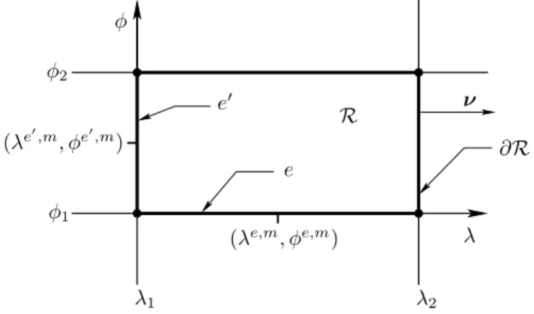
The general structure of our grid is shown in Figure 1, and its essential feature is the following. Every cell R is bounded by sides which lie either along a fixed latitude circle (φ = const.) or a fixed longitude circle (λ = const.). We have
R :=!λ1≤ λ ≤ λ2, φ1≤ φ ≤ φ2", (4.1)
as represented in Figure 2. In most cases, ∂R consists of the four sides of R. However, across special latitude circles we reduce the number of cells, so that the situation (for a reduction by ratio of 2) is as in Figure 3. In this case the boundary ∂R consists of five sides, (so that the intermediate point (λ3, φ2) is regarded as an additional vertex), and
even in this five-sided cell R every side satisfies the above requirement.
λ λ1 λ2 (λe,m, φe,m) φ φ1 φ2 (λe!,m , φe!,m ) ν R ∂R e e!
Fig. 2. Rectangular cellR as part of grid on S2
The length of a side e =!λ1 ≤ λ ≤ λ2, φ = const."equals (λ2− λ1) cos φ, while the
length of a side e!=!φ
1≤ φ ≤ φ2, λ = const."is φ2− φ1. Consequently, the area AR
of the cell R is AR= ' λ2 λ1 dλ' φ2 φ1
cosφ dφ = (λ2− λ1)(sin φ2− sin φ1).
4.2. Geometry-compatible discretization of the divergence operator
Given any rectangular domain R of the form (4.1), the approximate flux divergence is now derived as an approximation of the integral of the flux along the boundary ∂R, divided by its area, as follows:
Phi3 λ λ1 λ2 λ3 (λe,m, φe,m) φ φ1 φ2 (λe!,m, φe!,m) ν R ∂R e e!
Fig. 3. Five-sided rectangular cellR (on southern hemisphere of S2)
% ∇T· F(x, u) &approx = IR AR, IR =%, ∂R F(x, u) · ν ds&approx, (4.2) where ds is the arc length along ∂R and ν is the outward-pointing unit normal to ∂R ⊂ S2. In the limit λ
2, φ2 → λ1, φ1 the approximation (4.2) to the divergence term
approaches the exact value (1.2).
We need to check that the geometric compatibility condition (2.2) is satisfied for the approximate flux divergence. This requirement will be taken into account in formulating our finite volume scheme for (1.3).
Consider now the actual evaluation of the term IR defined in (4.2) and consider the
cell shown in Figure 2, under the assumption that u = u(λ, φ, t) is smooth on R. We propose to approximate the flux integral along each edge of R in the following way. As in Section 2, let us decompose the flux into its (λ, φ) components:
F(x, u) = Fλ(λ, φ, u)iλ+ Fφ(λ, φ, u)iφ.
On each side the integration is carried out by (i) taking midpoint values of the appro-priate flux component, and (ii) using the correct arc-length of the side. We designate the midpoints of the edge e as λe,m = (λ
1+ λ2)/2 and φe,m = φ1 (see Figure 2), and
likewise for the edge e!.
Throughout the rest of this section we restrict attention to the gradient flux vector constructed in Claim 2.2. In particular, it comprises the class of homogeneous flux vectors, given by (2.3)–(2.4).
Taking u as constant u = ue,m along the side e ∈ ∂R, the total approximate flux is
given by
- ,
e
where e1, e2 are, respectively, the initial and final endpoints of e (with respect to the
sense of the integration).
Summing up over all edges we obtain:
Claim 4.1 (Discrete geometry-compatibility condition.) Consider the gradient flux vector constructed in Claim 2.2. Then, if u ≡ const., IR= 0, so that
/
∇T · F(x, u)
0approx
= 0,
and thus a discrete version of the divergence-free condition (2.2) holds.
Remark 4.2 The claim above applies to gradient flux vectors in Claim 2.2, and, in par-ticular, to homogeneous flux (2.3)–(2.4). On the other hand, for a more general geometry-compatible flux F(x, u), such a result can be obtained only if the dependence on x is integrated exactly along each side, a requirement that must be imposed on the scheme. 4.3. Godunov-type approach to the numerical flux
We continue to deal with the gradient flux given in Claim 2.2. We assume different (constant) values of u = u(λ, φ, t) in grid cells and evaluate the numerical flux values at each edge from the solution to a Riemann problem with data comprising these values u(λ, φ, t) in the cells on either side of that edge. At the midpoint (λe,m, φe,m) of each side e
we solve the Riemann problem in a direction perpendicular to e, and denote the resulting solution ue,m. The corresponding fluxes are then evaluated as F(λe,m, φe,m, ue,m).
We can split Eq. (1.3) by invoking the explicit form of the divergence (1.2), getting ∂u
∂t + 1 cos φ
∂
∂λFλ(λ, φ, u) = 0 for the side e
!: λ = λ 2, (4.4)λ ∂u ∂t − 1 cos φ ∂ ∂φ % Fφ(λ, φ, u) cos φ &
= 0 for the side e : φ = φ2, (4.4)φ
Consider two adjacent cells, as in Figure 4 or in Figure 5. By fixing φ = φe,m (resp. λ =
λe,m) in (4.4)
λ(resp. (4.4)φ) we can evaluate u = ue,mas a one-dimensional solution at
λ = λe,m (resp. φ = φe,m).
λ1 λ2 λ3 φ1 φ2 φe!,m u = u L u = uR u = ue!,m M e!
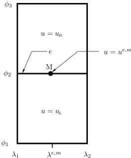
λ1 λe,m λ2 φ1 φ2 φ3 u = uL u = uR u = ue,m M e
Fig. 5. Two φ-adjacent cells with constant states uL, uR
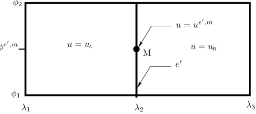
We include here some remarks that will be useful in the implementation of the scheme. Consider an homogeneous flux vector as in Claim 2.1 so that its components are given by (2.4). Suppose that u(λ, φ, tn) = uL (resp. u(λ, φ, tn) = uR) in the cell
!
λ1 < λ<
λ2, φ1 < φ < φ2"(resp. !λ2 < λ < λ3, φ1 < φ < φ2
1
), as in Figure 4. At the point M (λe!,m, φe!,m) Eq. (4.4)
λtakes the form
∂u
∂t + tan φ
e!,m ∂
∂λ %
f1(u) cos λ + f2(u) sin λ
&
−∂λ∂ f3(u) = 0. (4.5)
Setting
g(λ, u) = tan φe!,m%f1(u) cos λ + f2(u) sin λ
&
− f3(u), (4.6)
we see that equation (4.5) is the scalar one-dimensional conservation law ∂u
∂t + ∂
∂λg(λ, u) = 0, t≥ tn (4.7) subject to the initial data u = uL (resp. u = uR) for λ < λ2 (resp. λ > λ2).
Likewise, we repeat the former analysis for φ-adjacent cells by taking the constant states u(λ, φ, tn)=uL, u(λ, φ, tn)=uRin cells
!
λ1<λ<λ2, φ1<φ < φ2",!λ1<λ<λ2, φ2<φ<φ3",
as depicted in Figure 5. At the point M(λ = λe,m, φ = φ
2), the equation (4.4)φthen takes
the form ∂u ∂t + 1 cos φ ∂ ∂φ %
− sin λe,mcos φf1(u) + cos λe,mcos φf2(u)
&
= 0. (4.8) We then set the φ-flux function
k(φ, u) =%− sin λe,mf1(u) + cos λe,mf2(u)
&
so that equation (4.8) is the scalar one-dimensional conservation law ∂u ∂t + 1 cos φ ∂ ∂φk(φ, u) = 0, t≥ tn (4.10) subject to the initial data u = uL (resp. u = uR) for φ < φ2 (resp. φ > φ2).
4.4. Solution to the Riemann problem
The solution at the discontinuity λ=λ2 at the initial time t = tn is given by the
Riemann solution to (4.4)λ. For simplicity of the presentation we specialize here to the
flux (4.7). Since the dependence of g(λ, u) on λ is smooth, this solution is obtained by fixing λ = λ2, thus solving the classical conservation law
∂u ∂t +
∂
∂λg(λ2, u) = 0, t≥ tn (4.11) subject to the initial jump discontinuity of u.
We denote this solution by u2,m. Observe that the flux g(λ, u) in (4.11) is in
gen-eral non-convex. The Riemann solution may therefore consist of sevgen-eral waves. It is a self-similar solution depending only on the slope (λ − λ2)/(t − tn). The value u2,m is
the value along the line λ=λ2. It therefore corresponds either to a sonic wave, namely
g!(λ2, u2,m)=0, or to an “upwind value” u=uL (resp. u=uR) in the case where all waves
propagate to the right (resp. left).
Actually, the procedure for solving the Riemann problem in the case of a nonconvex flux function g(λ2, u) is well-known and goes back to classical works by Oleinik and
others. We recall it here briefly. Assume first that uL<uR. Consider the convex envelope
of g, namely, the largest convex continuous function gc, over the interval [uL, uR], such
that gc≤g at all points. Clearly, gc=g in “convex sections” of the graph of g, while it
consists of linear segments when gc<g. It is easy to see that the “convex segments”,
where g=gc, represent rarefaction waves (in the full Riemann solution) while the linear
segments represent jumps (i.e., shock waves). In particular, the solution u2,m is given by
the following formula:
u2,m= vmin, where g(λ2, vmin) ≤ g(λ2, v) for all v ∈ [uL, uR]. (4.12)
There are in fact three possibilities for this solution:
a) uL< u2,m< uR, which implies that g!(λ2, u2,m) = 0 (a sonic point).
b) u2,m= u
L, the whole wave pattern moves to the right.
c) u2,m= u
R, the whole wave pattern moves to the left.
Similarly, in the case uL>uR, we construct the “concave envelope” of g, namely, the
smallest concave continuous function gc such that gc≥g. Again the linear segments
cor-respond to jump discontinuities while the concave segments (g=gc) correspond to
rar-efaction waves. The solution to the Riemann problem is now given by u2,m=v
max, where
g(λ2, vmax)≥g(λ2, v), v∈ [uR, uL]. As above, there are three possibilities for the solution
(sonic, left-upwind, or right-upwind).
Replacing in the foregoing analysis the λ-flux function g(λ2, u) by the φ-flux function
k(φ2, u), the equation (4.10) reads
∂u ∂t +
∂ ∂φ
%
− sin λ2,mf1(u) + cos λ2,mf2(u)
&
We get the Riemann solution to (4.13) in the three cases a), b), c) as above. 4.5. Convergence proof
The computational elements (“grid cells”) are denoted in [2] by K. Their sides are denoted by e and the flux function across e is given by fe,K(u, v), where u is the (constant)
value in K and v is the value in the neighboring cell (sharing the same side e) Ke. In
our grid of the sphere, some cells are actually pentagons; these are the cells whose lower-latitude side (along a lower-latitude φ = const) borders the two higher-lower-latitude sides of the two lower-latitude neighbor cells, as shown in Figure 3 for the southern hemisphere grid. For such cells, the lower-latitude side consists of two faces, each one of them common with one of the lower-latitude neighboring cells.
With this construction of the grid, we can check the conditions in [2] imposed on the numerical flux. It is important to keep in mind that we are dealing with the gradient flux vectors given by Claim 2.2.
Claim 4.3 (Convergence of the proposed scheme.) Consider the first-order finite volume scheme described above. Assume that the flux vector has the gradient form in Claim 2.2. Let fe,R(u, v) be the numerical flux calculated on the side e of the
computa-tional cell R, using (4.3), where the midpoint value of u is obtained from the Riemann solution. Then fe,R(u, v) satisfies the assumptions (5.5)-(5.7) of [2], and the numerical
solution converges to the exact solution as the maximal size of the grid cells shrinks to zero.
Proof. Consider the flux across a longitude side e : λ = λ2, which is given by Fλ in
the equation (4.4)λ. The procedure for integrating the flux across e is described by
(4.3), while in Subsection 4.4 the calculation of Fλ(λ2, φ2,m, u2,m) is described. It can be
summarized as follows.
First, the solution u2,m to the Riemann problem associated with equation (4.4) λis
found, assuming u, v to be the values on the two sides. However, note that Fλ depends
explicitly on φ, and to be precise we need to replace in (4.4)λthe mean value φ2,mby φ.
Thus, we find u2,m= u2,m(φ).
Clearly, in the case u = v we get identically u2,m(φ) = u = v and so the exact flux
satisfies
Fλ= Fλ(λ2, φ, u2,m)
and its integration will give exactly the approximate value fe,K(u, v) = −(h(e2, u2,m) − h(e1, u2,m)),
as in (4.3). Thus, condition (5.5) in [2] is satisfied.
Clearly, the conservation property (5.6) is satisfied even with the approximate defini-tion.
Also, the flux as defined in (4.3) makes it easy to check (5.7), as the flux is independent of φ and the monotonicity is thus a result of general properties of the Riemann solver (even for nonconvex fluxes). For example, if u < v, one considers the convex envelope of Fλ, as defined in (4.4)λ(with φ = φ2,m) and then considers u2,m as the minimal value
on this envelope (over [u, v]). Clearly changing u upward will either change u2,m upward
or leave it unchanged. This completes the proof. ! 5. Second-order extension based on the GRP solver
To improve the order of accuracy, we consider again the cell λ1<λ<λ2, φ1<φ<φ2 and
assume that u is linearly distributed there. We use uL,λ, uL,φ(resp. uR,λ, uR,φ) to denote the
slopes in the cell to the left (resp. right) of the side λ=λ2. We also denote by uL(φ) (resp.
uR(φ)) the limiting value (linearly distributed) of u at λ=λ2− (resp. λ=λ2+). Clearly,
the solution to the Riemann problem across the discontinuity is a function of φ, and we denote it by u2,m(φ), which conforms to our notation in Subsecion 4.4 above (where
u was constant on either side of the discontinuity). The value of u2,m(φ) is obtained
by solving the Riemann problem associated with Eq. (4.4)λwith φ2,m replaced by φ,
subject to the initial data uL(φ), uR(φ). Restricting to the middle point φ = φ2,m, the
solution u2,m(φ2,m) (at λ = λ2,m) is in one of the three categories listed above (i.e., sonic,
left-upwind, right-upwind). By continuity, the solution u2,m(φ) will still be in the same
category for φ − φ2,m sufficiently small. The solution at (λ2,m, φ2,m) varies in time and
the GRP method deals with the determination of its time-derivative at that point. Accounting for the variation of the solution over a time interval enables us to modify the Godunov approach to the determination of edge fluxes , as presented in Section 4.3. We assume that the flux vector depends explicitly on x, as in (2.1). In what follows we use for simplicity the “imbedded” notation x = (x1, x2, x3) for a point on the sphere (see
the Introduction), along with the corresponding spherical coordinates λ, φ. We further assume that the vector field Φ is given by the following extension of (2.3)
Φ(x, u) = ∇xh(x, u)
= q1(x1)f1(u) i1+ q2(x2)f2(u) i2+ q3(x3)f3(u) i3,
(5.1) The zero-divergence identity is obtained as a result of expressing Φ as a gradient ∇h in the sense of Claim 2.2.
For our choice of Φ such a representation of Φ as gradient of h is obtained when h is taken as
h(x, u) = r1(x1)f1(u) + r2(x2)f2(u) + r3(x3)f3(u) , (5.2)
and qj(xj) = r!j(xj), j = 1, 2, 3.
Using (1.2) together with the geometry-compatibility property, we get an explicit form of the conservation law (1.3) in our case as
∂u ∂t − sin λq1(x1) ∂ ∂φf1(u) + cos λq2(x2) ∂ ∂φf2(u) + tan φ%cos λq1(x1) ∂ ∂λf1(u) + sin λq2(x2) ∂ ∂λf2(u) & − q3(x3) ∂ ∂λf3(u) = 0. (5.3) The numerical approximation to this equation requires an operator splitting approach, where the derivatives with respect to φ and λ are considered separately. We note that such a splitting has already been implemented in the Godunov case, (4.4), in the most general case. In that case, no use has been made of the geometry-compatibility property. Indeed, this has no bearing on the first-order scheme since the solution to the Riemann problem is obtained by “freezing” the explicit dependence on λ, φ (and, in particular,
ignoring the terms involving the derivatives with respect to this explicit dependence). In the present (second-order) situation we proceed as follows.
The “λ-split” equation obtained from (5.3), is ∂u ∂t + tan φ 2,m%q 1(x1) cos λ ∂ ∂λf1(u) + q2(x2) sin λ ∂ ∂λf2(u) & − q3(x3) ∂ ∂λf3(u) = 0. (5.4) Note that the coefficients are retained as functions of λ and are not “frozen” at λ = λ2,m. This is of course due to the fact that in employing the GRP scheme we consider
λ-derivatives on either side of the edge, so as in any limiting analysis, we must first let λ→ λ2,m, then substitute λ = λ2,m.
The λ-edge flux function g(λ, u) (compare (4.6)), is now extended to g(x, u) as g(x, u) = tan φ2,m%q1(x1) cos λf1(u) + q2(x2) sin λf2(u)
&
− q3(x3)f3(u),
and the scalar one-dimensional conservation law under consideration is now rewritten as an equation with a source term (a balance law)
∂u ∂t + ∂ ∂λg(x, u) = Sλ, t > tn Sλ= tan φ2,m % f1(u) ∂ ∂λ ( q1(x1) cos λ)+ f2(u) ∂ ∂λ (
q2(x2) sin λ)&− f3(u) ∂
∂λq3(x3), (5.5) subject to the initial data (for u and its slope) uL(φ2,m), uL,λ (resp. uR(φ2,m), uR,λ) for
λ < λ2 (resp. λ > λ2). Observe that the equation is written in a “quasi-conservative
form”, which offers more convenience in the GRP treatment [3, Chap. 5]. The right-hand side term Sλ is just the result of the λ differentiation of the flux g(x, u). Obviously,
the geometry-compatibility condition implies that this source term should cancel out with the corresponding source term in the “φ-split” equation. The solution u2,m to the
Riemann problem is obtained by freezing the coordinate λ at its edge value, so that, in particular, the source term in (5.5) can be taken as zero at this stage.
In the framework of the GRP analysis, the source term Sλ is added to terms arising
from the piecewise-linear initial data, in producing the time-derivative of the solution u2,m(φ2,m) + ∂u
∂t(λ2,m, φ2,m, tn+) ∆t
2 , ∆t = tn+1− tn. As explained above, u2,m(φ2,m),
the solution to the associated Riemann problem, is obtained by using the “edge val-ues” uL(φ), uR(φ). It remains, therefore, to determine the instantaneous time-derivative
∂u
∂t(λ2,m, φ2,m, tn+), as is outlined below.
The time-derivative of u is given by ∂u ∂t(λ 2,m, φ2,m, t n+) = −um,λ ∂ ∂ug(x, u)|λ2,m,φ2,m,u2,m,
where the slope value um,λ is obtained by “upwinding”, determined by the associated
Riemann problem as follows (we start with the “easy” categories b), c) above). b) u2,m= u
L(φ2,m). Then, the wave moves to the right and we set
um,λ= uL,λ.
c) u2,m= u
R(φ2,m). Then, the wave moves to the left and we set
Finally, the first category deals with the sonic case. As noted above, it remains sonic in the neighborhood of φ2,m, so that we have there ∂
∂ug(x, u)|λ2,m,φ2,m,u2,m. The
time-derivative of u reduces therefore to ∂
∂tu(λ2, φ
2,m, t=t
n+) = 0.
Finally, the “φ-split” equation obtained from (5.3), is treated in analogy with the “λ-split” procedure outlined above.
6. Numerical tests
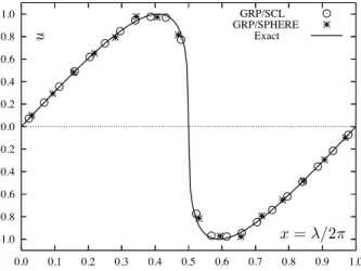
6.1. First test case: equatorial periodic solutions
Here, the conservation law takes the form (3.1) and the flux function and initial data are given by
f1(u) = f2(u) = 0, f3(u) = −2π (u2/2),
u(λ, φ, 0) = 2
sin λ, 0 < λ < 2π, 0 < φ < π/12, 0, otherwise.
(6.1) As discussed in Section 3 (see the discussion of solutions to (3.1)) it is clear that the solution here (as a function of λ) is identical to the periodic solution for the Burgers equation in R1, with periodic boundary conditions on [0 < x < 2π]. However, we compute
the numerical solution here on our spherical grid, and we need to check not only that it conforms with the one-dimensional case but that it does not “leak” beyond the band supporting the initial data. The results at the shock formation time ts= 1/2π are shown
in Figure 6 for ∆λ = 2π/16, in Figure 7 for ∆λ = 2π/32 and in Figure 8 for ∆λ = 2π/64. These GRP solutions to (4.7) clearly converge to the exact solution with refinement of the λ grid, and are comparable to the corresponding solution to the scalar conservation law in R1 with ∆x = 2π/22. -1.0 -0.8 -0.6 -0.4 -0.2 0.0 0.2 0.4 0.6 0.8 1.0 0.0 0.1 0.2 0.3 0.4 0.5 0.6 0.7 0.8 0.9 1.0 GRP/SCL GRP/SPHERE Exact x = λ/2π u
-1.0 -0.8 -0.6 -0.4 -0.2 0.0 0.2 0.4 0.6 0.8 1.0 0.0 0.1 0.2 0.3 0.4 0.5 0.6 0.7 0.8 0.9 1.0 GRP/SCL GRP/SPHERE Exact x = λ/2π u
Fig. 7. Exact, GRP/SCL and GRP/SPHERE (∆λ=2π/32) solutions to the IVP (6.1) at t = 1/2π
-1.0 -0.8 -0.6 -0.4 -0.2 0.0 0.2 0.4 0.6 0.8 1.0 0.0 0.1 0.2 0.3 0.4 0.5 0.6 0.7 0.8 0.9 1.0 GRP/SCL GRP/SPHERE Exact x = λ/2π u
Fig. 8. Exact, GRP/SCL and GRP/SPHERE (∆λ=2π/64) solutions to the IVP (6.1) at t = 1/2π
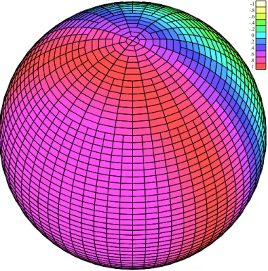
6.2. Second test case: steady state solutions
We refer to Corollary 3.3 and using the notation there we take the flux vector and initial data as:
f1(u) = u2/2, f2(u) = f3(u) = 0,
u(λ, φ, 0) = cos λ cos φ. (6.2) Using the terminology of Corollary 3.3 we see that the initial function is the “simplest” possible function, corresponding to g(x1) = x1.
As is shown in Figure 9, the numerical solution remains nearly unchanged in time after being subjected to integration up to t = 5 by the GRP scheme with constant time step ∆t = 0.05, the color maps of u(λ, φ, t) at the initial and final times are virtually indistinguishable. The shown grid has latitude step ∆φ = π/60, and an equatorial longitude step ∆λ = π/128. A measure udif f to the numerical solution error is defined
-1 -.8 -.6 -.4 -.2 0 .2 .4 .6 .8 1
Fig. 9. Steady-state initial data (and solution) to the IVP (6.2) at t = 5. Color map range scaled to (umin, umax) = (−0.998, 0.998).
as the area-weighted difference |u(λ, φ, 5) − u(λ, φ, 0)|, obtained by summation over all grid cells. In this case we obtained udif f = 0.0093, which is small relative to the full range
umax− umin = 2. Hence, the GRP scheme produces an approximation to the
steady-state solution u(λ, φ, t) = u(λ, φ, 0) over S2. This test case demonstrates that the scheme
computes correctly the time-evolution for the non-constant data (6.2), by calculating an approximately zero value for the flux divergence in computational cells.
6.3. Third test case: confined solutions
We take (as in Claim 2.2) Φ(x, u) = ∇h(x, u), where h(x, u) = ψ(x1)x1f1(u). The
function ψ(x1) is defined by ψ(x1) = 1, x1≤ 0, 1 − 6x2 1+ 8 √ 2x 3 1, 0 ≤ x1≤ √ 2 2 , 0, √2 2 ≤x1. (6.3)
The flux vector is then given by
F(x, u) = n(x) × Φ(x, u). The solution is clearly confined to the sector x1 ≤
√ 2
2 of the sphere. Its boundary is a
circle which intersects the meridian λ = 0 at φ = π 4.
The flux in the subdomain x1≤ 0 is given by
F(x, u) = n(x) × f1(u) i1,
so if we take the initial data as ψ(x1)u0(x1), where u0 is the steady state solution of
the second test case (and also the same f1(u)), the solution remains steady in that part,
namely, in x1 ≤ 0. Clearly, it evolves in time in the region 0 ≤ x1 ≤ √
2
2 , but vanishes
identically (for all time) if √2 2 ≤ x1.
The confined IVP was integrated in time up to t = 5 by the GRP scheme, using the same grid and time step as in the second test case (Subsection 6.2). The solution is represented by the color map in Figure 10. Comparing it to the corresponding initial map (not shown here), it seems nearly unchanged. In fact, the initial-to-final difference measure obtained is udif f = 0.0057, which indicates a nearly steady solution in the strip
0 < x1 <
7
1/2 . This test case demonstrates that the scheme computes correctly the time-evolution for the non-constant “confined” data (6.3).
-1 -.8 -.6 -.4 -.2 0 .2 .4 .6 .8 1
Fig. 10. Confined solution test case, with the IVP data to the IVP (6.3) at t = 5. Color map range scaled to (umin, umax) = (−0.998, 0.183).
Acknowledgments
The authors were supported by a research grant of cooperation in mathematics, spon-sored by the High Council for Scientific and Technological Cooperation between France and Israel, entitled: “Theoretical and numerical study of geophysical fluid dynamics in
general geometry”. This research was also partially supported by the A.N.R. (Agence Nationale de la Recherche) through the grant 06-2-134423 and by the Centre National de la Recherche Scientifique (CNRS).
References
[1] P. Amorim, P.G. LeFloch, and B. Okutmustur, Finite volume schemes on Lorentzian manifolds, Comm. Math. Sc. 6 (2008), 1059–1086.
[2] P. Amorim, M. Ben-Artzi, and P.G. LeFloch, Hyperbolic conservation laws on manifolds. Total variation estimates and the finite volume method, Meth. Appli. Analysis 12 (2005), 291–324. [3] M. Ben-Artzi and J. Falcovitz, Generalized Riemann problems in computational fluid dynamics,
Cambridge University Press, London, 2003.
[4] M. Ben-Artzi and J. Falcovitz, and P.G. LeFloch, Hyperbolic conservation laws on the sphere. The shallow water model, in preparation.
[5] M. Ben-Artzi, J. Falcovitz, and J. Li, Wave interactions and numerical approximation for two-dimensional scalar conservation laws, Comp. Fluid Dynamics J. 14 (2006), 401–418.
[6] M. Ben-Artzi and P.G. LeFloch, The well-posedness theory for geometry-compatible hyperbolic conservation laws on manifolds, Ann. Inst. H. Poincar´e : Nonlin. Anal. 24 (2007), 989–1008. [7] G.J. Haltiner, Numerical weather prediction, John Wiley Press, 1971.
[8] P.G. LeFloch, Neves W., and B. Okutmustur, Hyperbolic conservation laws on manifolds. Error estimate for finite volume schemes, Acta Math. Sinica (2009).
[9] P.G. LeFloch and B. Okutmustur, Hyperbolic conservation laws on spacetimes. A finite volume scheme based on differential forms, Far East J. Math. Sci. 31 (2008), 49–83.
[10] J. Li, S. Yang, and T. Zhang, The two-dimensional Riemann problem in gas dynamics, Pitman Press, 1998.


![[PDF] Formation avancé du langage Fortran | Cours informatique](data:image/gif;base64,R0lGODlhAQABAIAAAP///wAAACH5BAEAAAAALAAAAAABAAEAAAICRAEAOw==)