HAL Id: hal-02867917
https://hal.archives-ouvertes.fr/hal-02867917
Submitted on 15 Nov 2020HAL is a multi-disciplinary open access archive for the deposit and dissemination of sci-entific research documents, whether they are pub-lished or not. The documents may come from teaching and research institutions in France or abroad, or from public or private research centers.
L’archive ouverte pluridisciplinaire HAL, est destinée au dépôt et à la diffusion de documents scientifiques de niveau recherche, publiés ou non, émanant des établissements d’enseignement et de recherche français ou étrangers, des laboratoires publics ou privés.
Le binge drinking est-il toujours profitable à l’industrie
alcoolière ? Un modèle épidémique de la consommation
d’alcool
Milena Spach, Antoine Pietri
To cite this version:
Milena Spach, Antoine Pietri. Le binge drinking est-il toujours profitable à l’industrie alcoolière ? Un modèle épidémique de la consommation d’alcool. Revue Economique, Presses de Sciences Po, 2018, 69 (4), pp.635-646. �hal-02867917�
I
S HEAVY DRINKING ALWAYS PROFITABLE FOR ALCOHOL INDUSTRY?
A
N EPIDEMIC FRAMEWORK FOR ALCOHOL CONSUMPTIONAbstract
This article aims to provide a better understanding of the impact of heavy drinkers on the alcohol industry s profitability. At first glance, heavy drinking appears to improve alcohol s sales leading to an increase of profit. However, heavy drinking also involves fatal injuries and constitutes a shortfall for the industry. In this paper, we explore coexistence of these two forces through an epidemic model of alcohol use distinguishing light and heavy drinkers ( LH model). We find that there exists a level of alcohol consumption beyond which heavy drinkers represent a loss of profit for the alcohol industry. We calibrate our model with U.S. data for 2011 and we estimate that this threshold should be between 10.22 and 10.80 drinks per heavy drinking occasion. The implication of our result is twofold: the alcohol industry should set up more effective actions against the heaviest consumers, and consequently genuine collaborations with public authorities could exist for this fringe of population.
1. INTRODUCTION
Alcohol, tobacco and other drugs (e.g. cocaine, heroin) are specific goods in the sense that these substances are addictive, and involve health, social and economic costs (Anderson and Baumberg, 2006; WHO, 2014). Among them, alcohol consumption is ranked the fifth leading cause of death and disability and accounted for 5.9% of global mortality in 2012 (WHO, 2014). More generally, the social cost of alcohol to the European Union (E.U.) is 125bn in 2003, equivalent to 1.3% of GDP (Anderson and Baumberg, 2006). In response to these alarming figures, health authorities implement prevention actions in order to reduce alcohol consumption, especially for harmful drinkers – that is people who are risking their health or doing themselves potentially lethal damages. In parallel, alcohol industry sets up Responsible Drinking Programs (RDPs), promoting responsible and moderate alcohol consumption. However, scholars often point an existing conflict of interest between alcohol industry and public health because a large part of alcohol industry s sales comes from harmful drinkers (Baumberg, 2009). Indeed, RDPs are often used to promote new products, or are part of a public relations strategy to reduce criticism and potentially forestall government regulations, rather than to prevent alcohol excessive use (Pantani et al., 2012; Smith et al., 2014; Esser et al., 2016). Consequently, RDPs are often ineffective (Casswell et al., 2016) and alcohol industry devotes very little effort to assess the impact of these actions (Pantani et al., 2012; Esser et al., 2016). In this article we argue that the alcohol industry should take into account more seriously the fight against harmful drinkers because it may be in its best interests.
This is an english version of the article "Le binge drinking est-il toujours profitable à l’industrie
alcoolière ? Un modèle épidémique de la consommation d’alcool", published in Revue Economique
2018 69(4): pp.635-649.
https://www.cairn.info/revue-economique-2018-4-page-635.htm?contenu=resume
Miléna SPACH et Antoine PIETRI Université Paris 1, CES
In order to apprehend the spread of drug use in a given population, scholars turned to epidemic models to capture the co-evolution between light users ( L ) and heavy users ( H ) (Behrens et al., 1999). Like an infectious disease, drug use largely depends on the prevalence of light and heavy users among the population. These models (hereafter LH models) describe two groups of users (L and H) evolving according to three kinds of flows: the initiation flow representing new consumers, the escalation rate depicting the rate at which light users become heavy ones, and the exit rate capturing the share of users who stop using drugs. These epidemic models are mainly used in the case of cocaine (Behrens et al., 1999; Caulkins et al., 2010) or tobacco (Massin, 2012), and allow to highlight the existence of feedbacks generated by consumers themselves. First, light users generate a positive feedback on initiation because new consumers typically look for social integration. Second, heavy users yield negative feedback on initiation due to the bad publicity provided by damaged drug users. All these flows (initiation, escalation and exit) shape LH models.
If this framework seems correctly fitted with tobacco and cocaine s consumptions, it fails to depict the spread of alcohol uses. Compared to other drugs, two original key features can be drawn for the alcohol case: i) the high severity of short-term risks related to heavy consumption and ii) the social attractiveness of heavy drinkers. First, alcohol mortality burden can be divided into short-term deaths, resulting from a single consumption episode, and long-term deaths, arising from patterns of alcohol consumption (e.g. cancers, neuropsychiatric diseases, cardiovascular diseases). Short-term deaths mainly comprise intentional (e.g. self-inflicted injuries, homicides) and unintentional (e.g. motor vehicle collisions, poisonings, falls) injuries. For people aged 15-64 living in the E.U. in 2004, both intentional and unintentional injuries represent 32% of alcohol-attributable deaths (Rehm et al., 2012). Heavy drinking is the critical feature in determining the risk of fatal injury (Li et al., 1994). More precisely, heavy drinking corresponds to binge drinking which can be defined as consuming 60+ grams of pure alcohol per day for men (the equivalent of at least 5 standard drinks of 12 g pure alcohol) and 40+ grams for women (WHO, 2014). Consequently, short-terms deaths are much more widespread than in cocaine or tobacco s cases where mortality mainly results from long-term consumption. Second, contrary to heavy users in traditional LH models, heavy drinkers may generate a positive feedback on the escalation rate. Indeed, especially for young people, binge drinking may be socially valorized and considered as a status symbol (Walters et al., 2013). This point differs from other drugs where heavy users always have a deterrent effect on initiation (Massin, 2012). As a result, there is a need for an adjusted epidemic framework to provide a better understanding of the binge drinking phenomenon.
In this article we propose a modified LH model corresponding more accurately to alcohol use. Our model contains three major changes with respect to the literature. First, we modify the temporal horizon of the model in the sense that our main line of interest is the impact of short-term risks associated with heavy drinking. As a result, we provide a two-period LH model. Second, apart from pathological cases, heavy drinking requires an occasion (e.g. a specific day, friends reunions).
Outside this occasion heavy drinkers consume moderate doses of alcohol. Therefore, we consider that each period can be split into binge-drinking episodes and daily moderate consumption. Third, we integrate an endogenous escalation rate accounting for the social attractiveness of heavy drinkers.
Following Massin (2012) we implement the LH framework with an offer side, in our case alcohol industry . In accordance with standard microeconomic analysis, we consider a maximizing-profit agent and we analyze the impact of heavy consumption on its maximizing-profit. This integration allows us to study if heavy drinking is always profitable for the alcohol industry. Starting from the point that alcohol industry is interested in maximizing its profit, heavy drinkers have an ambivalent impact. On the one hand, because industry is driven by the need to sell as much as it possibly can ,1 heavy
drinking increases immediate profit. In fact, heavy drinkers represent 50% of sales of the alcohol industry in high income countries, 63% for middle income countries (Casswell et al., 2016). Also, the 20% heaviest drinkers consume 90% of total alcohol in Hungary, 73% in U.S., 63% in England, and 50% in France (OECD, 2015b). On the other hand, due to inherent risks of fatal injuries, and because killing the customer is not good for business (Earl, 2005, p. 148), heavy drinkers diminish future profits through a loss of consumers.
By using a modified LH model, we find that beyond a threshold of alcohol consumption, the risk of fatal injuries may outweigh the benefits of the alcohol industry. Then, pursuant to the U.S. Behavioral
Risk Factor Surveillance System (BRFSS) data for the year 2011, we estimate this threshold may be
between 10.22 and 10.80 drinks (or 143.08 – 151.2 grams of pure alcohol) per heavy drinking occasion. Our article can be seen as a modest theoretical contribution on why alcohol industry has an interest to genuinely combat heaviest consumptions.
The paper proceeds as follows. Our theoretical model is presented in Section 2. In Section 3, we calibrate our model with U.S. data and we conclude in Section 4.
2. A TWO-PERIOD ‘LH’ MODEL
In order to focus on short-term risks associated with alcohol consumption, we use a two-period LH model. A different way of seeing things would be to say that our model considers myopic agents abstracting for long-term considerations.
2.1. General description of the model
LH models typically consider a given population differentiated into two groups: light drinkers ( ) and heavy ones ( ). This population evolves between period 1 and period 2 as depicted in Figure 1.
1 The Guardian, 22 January 2016, Problem drinkers account for most of alcohol industry s sales, figures
reveal . Link: https://www.theguardian.com/society/2016/jan/22/problem-drinkers-alcohol-industry-most-sales-figures-reveal (accessed March 15, 2017).
Figure 1. Diagram flow for the two-period LH model
Figure 1 distinguishes three kinds of flows. First, the initiation, , represents the new (light) consumers at the end of the first period. For the sake of clarity, we assume that the number of new light consumers is not influenced by short-term risks and is considered as exogenous. Second, the escalation parameter, , captures the flow of light drinkers who become heavy ones. This flow corresponds to a desire of social interactions considering the more or less appealing nature of alcohol (Mubayi and Greenwood, 2013). Following Behrens et al. (1999), we use the Markov assumption stating that flows from heavy to light drinkers are indistinguishable from those from light to heavy drinkers. Third, the exit parameters, and , measure the number of drinkers who stop consuming, because of death or ceasing use (e.g. pregnancy). Their value hinge upon individual short-term risks related to alcohol consumption. Flows are summarized in the following system:
Where is a positive parameter capturing the number of new light consumers at the end of the first period , is the probability of death for a j-drinker, and are parameters measuring the impact of the individual risk. In particular for the only reason for stopping alcohol use is death. On stark contrast, for all values higher than one, a share of drinkers quits drinking as a precaution, typically because they fear for their lives. Last, measures the weight attached to the desire of social interactions which positively depends on the share of heavy drinkers in the total population, . It should be noticed that may be either positive – if heavy drinking is socially valorized – or negative – if, for example, heavy drinkers are composed of marginalized people. This corresponds to the distinction between social drinkers and problem drinkers provided by Manthey et al. (2008).
Considering Figure 1 and , the evolution of the number of drinkers between period 1 and period 2 is defined by the following equations:
2.2. Alcohol consumptions and short-term risks related
Short-term risks associated with alcohol are non-uniformly distributed in a period and are mostly concentrated in binge drinking episodes (Li et al., 1994). As a result, we divide each period in a fixed share of binge drinking episodes depending on cultural and social factors . In the rest of the period, , there is no special occasion and drinkers have a daily moderate consumption. During a period, light drinkers always have the same (low) level of alcohol consumption, . On stark contrast, heavy drinkers change their consumption from during daily moderate consumption to during binge drinking episodes . As a result, for each period , the total level of alcohol consumption is defined as follows:
However, heavy drinkers have a negative external effect in the sense that they generate risks of fatal injuries for both type of drinkers ( and ). Let be the global risk of fatal injuries related to excessive consumption during festive episodes at the end of the first period. Following Borges et al. (2006) and Rehm et al. (2012), we consider an exponential relation between the global risk of fatal injuries and the level of heavy consumption such as:
Where is a positive parameter. This risk can be decomposed as the weighted sum of individual risks borne by each kind of drinkers: , where is the probability of death for a -drinker, . Let be the relative risk for a heavy drinker compared to a light one
. We can deduce from the following two relations:
2.3. The behavior of the alcohol industry
Following Massin (2012) we consider a profit-maximizing producer, the alcohol industry , whose profit is depicted by:
Where and are exogenous and respectively correspond to the price and the cost of one unit of alcohol, and is the discounted rate in our discrete two-period LH model. The exogeneity of and finds its justification in two elements: i) the price of alcohol is often fixed by the regulator and ii) our temporal horizon is the short-term, thus assuming stable production costs seem quite reasonable.
This paper aims to question the nature of the link between heavy drinking and profit. In particular heavy drinkers constitute a shortfall for the alcohol industry if According to equation , it would involve:
Inequality means that an increase in the level of heavy drinking is costly for the alcohol industry if gains realized during the first period – due to its increase – are inferior to actualized losses related to the decrease of alcohol sales in period two – due to higher short-term risks. Using , ,
and , we can rearrange as follows:
We face a computational difficulty related to the use of the exponential relation between the global risk of fatal injuries, , and . In order to isolate on the left-hand side, we use the Lambert W function , noted , where is the inverse function . It should be noticed that because , is a real number, and . In order to stay tractable and without loss of generality, we assume a unitary population at period 1 such as . We deduce from
the following threshold:
Proposition: In a two-period LH model addressing alcohol use, there is always a threshold of heavy drinking beyond which heavy drinkers represent a loss of profit for the alcohol industry. This threshold is given by .
Proof. We know that the level of heavy drinking is a positive number such as and, by definition of the Lambert W function , , and . As a result, is a finite number and it is always possible to pick a value of such as holds.
The proposition states that, from a theoretical perspective, there always exists a threshold beyond which heavy drinking damages the profit of the alcohol industry. The third section proposes to estimate the value of this threshold for the 2011 U.S. case.
3. CALIBRATION WITH 2011 UNITED STATES DATA
We use 2011 U.S. data to calibrate the value of the parameters of our model. Levels of alcohol consumption came from the 2011 Behavioral Risk Factor Surveillance System (BRFSS). The BRFSS is a state-based random-digit-dial telephone survey of people aged ≥18 years, which is conducted monthly in all states, the District of Columbia, and three U.S. territories. BRFSS collects self-reported data on health conditions and risk behaviors. Binge drinking was defined as consuming ≥5 (men) or ≥4 (women) drinks per occasion. Data were weighted to be representative of state populations2. Using the
2011 BRFSS, Kanny et al. (2013) stated that binge drinkers represent 18.4% of the U.S. population. Binge drinkers reported 4.2 occasions of binge drinking by month, with an average of 7.7 drinks by binge drinking episode. It should be noted that for the U.S. one standard drink is equal to 14 grams of pure alcohol. In order to shape our model to the available data, let the unit of alcohol be a drink and the period be a year. According to the findings of the study conducted by Latino-Martel et al. (2011) in some developed countries (UK, Australia, Denmark, France, etc.), we define daily moderate consumption as 2.5 drinks per day. Finally, we approximate the discount rate by the 2011 U.S. inflation rate (2.962%).
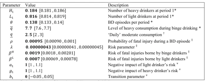
In 2011, the percentage of fatal injuries in the U.S. was 0.06%, and according to Guérin et al. (2013) the percentage of injuries attributable to alcohol consumption reaches 21.82%. The probability of dying from a fatal injury caused by alcohol per year is 0.01% and 0.095% per binge drinking episode. By doing so, we assume that fatal injuries caused by alcohol are only related to festive episodes, but both heavy drinkers and moderate ones have a probability of fatal injury of and , respectively. Following the study conducted by Borges et al. (2006) on several countries (Canada, Sweden, New Zealand, etc.), we consider that the relative risk between a consumption higher than 6 drinks and a consumption around 2-3 drinks equals 2.59 . Using equations and , we get and .We did not find documented values for and . As a result, we consider the most basic case in which (exit flows consist entirely of deaths) and (heavy drinking is neither attractive nor repulsive). All the values of the parameters are summarized in Table 13.
2 Extensive details about the BRFSS and its methods are available at www.cdc.gov/brfss (accessed March 01,
2017).
Table 1. Parameters of the model for the case of the United States in 2011
Parameter Value Description
Number of heavy drinkers at period 1* Number of light drinkers at period 1* BD episodes per period *
Level of heavy consumption during binge drinking * Daily moderate consumption †
Probability of fatal injury during a BD episode § Risk parameter §
Risk of fatal injuries borne by binge drinkers §
Risk of fatal injuries borne by light drinkers §
1 [1 , 1.1] Negative impact of light drinker s risk
1 [1 , 1.1] Negative impact of heavy drinker s risk
0 Transition parameter
* Ranges of values are 95% confidence interval (Kanny et al., 2013).
† Ranges of values are defined by Latino-Martel et al. (2011).
§ The lower bounds and the higher bounds are defined considering the minimum and maximum of fatal injury rates during the
period 2009-2013 calculated with data of the Centers for Disease Control and Prevention. We choose the fluctuating range such as the amplitude reaches 0.1.
We use a Monte Carlo-like approach in order to test the sensitivity of our result considering the ranges of values of the parameters used. We randomly and simultaneously simulated all parameters 10,000 times to obtain a consistent fluctuating range for the threshold highlighted in . According to our model calibrated with U.S. data, the threshold is 10.6 drinks (or 148 grams of pure alcohol) fluctuating into 10.22 – 10.80 drinks (or 143.08 – 151.2 grams of pure alcohol). This threshold is higher than the average number of drinks (7.7 drinks) consumed by binge drinkers during festive episodes in the U.S. in 2011. However, this figure disregards the variance of the average number of drinks. In fact, the intensity of binge drinking varies largely across socioeconomic data (Kanny et al., 2013). A salient illustration is provided by Dawson et al. (2010). With a representative population sample of U.S. drinkers, they show that, according to the type of disorder, people subject to alcohol use disorder report an average number of drinks included in a range between 9.4 and 15.4 per festive episodes. In the 2011 BRFSS, 3% of the drinking population consumed more than 10 drinks during a binge drinking episode, with an average of 15.86 drinks. According to our model these drinkers would represent a loss of profit for the U.S. alcohol industry.
Finally, it should be noticed that data from the BRFSS are self-reported and thus suffer from underreport, especially for binge drinking (Kanny et al., 2013; WHO, 2014). This is due to recall bias, social desirability response bias, and nonresponse bias (Stockwell et al., 2004). These biases probably imply a level of higher than 7.7 and a lower threshold as defined in . Consequently, results exhibited here are likely underestimated.
4. CONCLUSION
In this article we argue that, due to the short-term risks of fatal injuries, heavy drinkers may represent a loss of profit for the alcohol industry. We use a two-period LH model and we find that
there always exists a threshold of alcohol consumption during festive episodes beyond which heavy drinkers represent a shortfall for the alcohol industry. Regarding the U.S. case in 2011, the threshold estimated equals 10.6 drinks (or 148 grams of pure alcohol), fluctuating into 10.22 – 10.80 drinks (143.08 – 151.2 grams of pure alcohol) per heavy drinking occasion. Then, in order to maximize profits, alcohol industry would have an interest to limit alcohol consumption of heavy drinkers exceeding this threshold.
In our opinion, our results have two main implications. First of all, alcohol industry should take into account more seriously that a portion of heavy drinkers are bad for business and should set up more effective actions to face this loss of profit. However, as pointed by Esser et al. (2016, p. 711, brackets are ours): the alcohol industry did not report evaluation for nearly two third (63%) of its actions [to reduce drink driving from 1982 to May 2015]. Among the reported evaluations, none were rigorous […] . This lack of meticulousness shows that heavy drinking is currently not considered as a real issue for the industry. Yet, our results suggest that it should be the case. The second implication regards collaborations between public health and alcohol industry. We find that tackling (highly) excessive drinking through Public-Private collaboration may be a win-win strategy, as suggested by the OECD (2015a) report. Nonetheless, it should be noted that our results also indicate that for all drinkers consuming less than , the alcohol industry has interest to increase their level of alcohol use until the threshold. In this case, the conflict of interest is such the alcohol industry cannot afford to be [public authorities ] friend (Caswell et al. 2016, p. 663, brackets are ours). Consequently, a win-win collaboration may be reachable only for the heaviest drinkers.
Finally, this article can be characterized as a modest theoretical expansion of works conducted by Behrens et al. (1999), Caulkins et al. (2010), and Massin (2012) for the case of alcohol use. Further extensions of this work may be envisaged in future research. First, the temporal horizon of the model may be extended to capture long term-risks associated to alcohol use (e.g. cancers or cardiovascular diseases) and cohort-related effects. By doing so, heavy consumptions would represent a higher shortfall for the alcohol industry in the sense that the global risk ( increases. Therefore, by extending the temporal horizon of the model, we would find that alcohol industry should be more prone to implement effective actions to fight against heavy drinking. Second, a treatment stage may be implemented to account for people willing to stop consumption. Third, it would be interesting to distinguish for various age groups and other countries in order to study the impact of different patterns of drinking. For example, social drinking is a key feature of college drinking ( but seems less relevant for other populations (probably negative ). In the same vein, the threshold defined in is likely to be different between high income countries (low ) and middle income countries (high ) (Casswell et al., 2016), but also within high income countries, for example between Southern Europe (e.g. France, Italy) where binge drinking is not a common practice (low ) and Northern Europe (e.g. U.K., Sweden, Latvia) (high ) (OECD, 2015b).
APPENDIX A. Details concerning the value of the parameters described in Table 1
Parameters and are directly picked in previous works or studies as mentioned in Table 1.
Concerning parameters associated with short-term risks and :
Following equation , we have and thus
Following equation ,
.
Following equation , .
REFERENCES
Anderson, P., Baumberg, B. (2006). Alcohol in Europe. London: Institute of Alcohol Studies, 2, 73-75. Baumberg, B. (2009). How will alcohol sales in the UK be affected if drinkers follow government
guidelines? Alcohol and alcoholism, 44(5), 523-528.
Behrens, D.A., Caulkins, J.P., Tragler, G., Haunschmied, J.L., Feichtinger, G. (1999). A dynamical model of drug initiation: Implications for treatment and drug control. Mathematical Biosciences, 159(1), 1-20.
Borges, G., Cherpitel, C., Orozco, R., Bond, J., Ye, Y., Macdonald, S., Rehm, J., Poznyak, V. (2006). Multicentre study of acute alcohol use and non-fatal injuries: data from the WHO collaborative study on alcohol and injuries. Bulletin of the World Health Organization, 84(6), 453-460.
Caulkins, J.P., Feichtinger, G., Tragler, G., Wallner, D. (2010). When in a drug epidemic should the policy objective switch from use reduction to harm reduction? European Journal of Operational
Research, 201(1), 308-378.
Casswell, S., Callinan, S., Chaiyasong, S., Viet Cuong, P., Kazantseva, E., Bayandorj, T., Huckle, T., Parker, K., Railton, R., Wall, M. (2016). How the alcohol industry relies on harmful use of alcohol and works to protect its profit. Drug and Alcohol Review, 35(6), 661-664.
Dawson, D.A., Saha, T.D., Grant, B.F. (2010). A multidimensional assessment of the validity and utility of alcohol use disorder severity as determined by item response theory models. Drug and
Alcohol Dependence, 107(1), 31-38.
Earl, P.E. (2005). Review of the book The Economics of Sin: Rational Choice or No Choice at all? by Cameron, S., Elgar, E. 2002. Journal of Economic Psychology, 26(1), 147-149.
Esser, M.B., Bao, J., Jernigan, D.H., Hyder, A.A. (2016). Evaluation of the evidence base for the alcohol industry s actions to reduce drink driving globally. Journal Information, 106(4), 707-713. Guérin, S., Laplanche, A., Dunant, A., Hill, C. (2013). Alcohol-attributable mortality in France. The
11/11 Kanny, D., Liu, Y., Brewer, R.D., Lu, H. (2013). Binge Drinking – United States, 2011. In: Centers for Disease Control and Prevention (Eds.), Health Disparities and Inequalities Report – United
States, 2013. Morbidity and Mortality Weekly Report.
Latino-Martel, P., Arwidson, P., Ancellin, R., Druesne-Pecollo, N., Hercberg, S., Le Quellec-Nathan, M., Le-Luong, T., Maraninchi, D. (2011). Alcohol consumption and cancer risk: revisiting guidelines for sensible drinking. Canadian Medical Association Journal, 183(16), 1861-1865. Li, G., Smith, G.S., Baker, S.P. (1994). Drinking behavior in relation to cause of death among US
adults. American Journal of Public Health, 84(9), 1402–1406.
Manthey, J.L., Aidoo, A.Y., Ward, K.Y. (2008). Campus drinking: an epidemiological model. Journal
of Biological Dynamics, 2(3), 346-356.
Massin, S. (2012). Is harm reduction profitable? An analytical framework for corporate social responsibility based on an epidemic model of addictive consumption. Social Science &
Medicine, 74(12), 1856-1863.
Mubayi, A., Greenwood, P.E. (2013). Contextual interventions for controlling alcohol drinking. Mathematical Population Studies, 20(1), 27-53.
OECD (2015a). Tackling Harmful Alcohol Use. Economics and Public Health Policy.
OECD (2015b). Consommation d'alcool chez les adultes, dans Panorama de la santé 2015 : Les
indicateurs de l'OCDE. Éditions OCDE. Paris.
Pantani, D., Sparks, R., Sanchez, Z.M., Pinsky, I. (2012). Responsible drinking programs and the alcohol industry in Brazil: Killing two birds with one stone? Social Science & Medecine, 75(8), 1387-1391.
Rehm, J., Shield, K.D., Rehm, M.X., Gmel, G., Frick, U. (2012). Alcohol consumption, alcohol
dependence and attributable burden of disease in Europe. Potential gains from effective interventions for alcohol dependence. Toronto: Centre for Addiction and Mental Health (CAMH).
Smith, K.C, Cukier S., Jerningan D.H. (2014). Defining strategies for promoting product through drink responsibly messages in magazine ads for beer, spirits and alcopops. Drug and Alcohol
Dependence, 142, 168-173.
Stockwell, T., Donath, S., Cooper-Stanbury, M., Chikritzhs, T., Catalano, P., Mateo, C. (2004). Under-reporting of alcohol consumption in household surveys: a comparison of quantity-frequency, graduated-frequency and recent recall. Addiction, 99(8), 1024-1033.
Walters, C.E., Straughan, B., Kendal, J.R. (2013). Modelling alcohol problems: total recovery. Ricerche di Matematica, 62(1), 33-53.