Mobility reduction and apparent activation energies produced by hopping transport in the presence of Coulombic defects

HAL Id: hal-00437671

https://hal.archives-ouvertes.fr/hal-00437671

Submitted on 11 Feb 2010

HAL is a multi-disciplinary open access archive for the deposit and dissemination of sci-entific research documents, whether they are pub-lished or not. The documents may come from teaching and research institutions in France or abroad, or from public or private research centers.

L’archive ouverte pluridisciplinaire HAL, est destinée au dépôt et à la diffusion de documents scientifiques de niveau recherche, publiés ou non, émanant des établissements d’enseignement et de recherche français ou étrangers, des laboratoires publics ou privés.

Mobility reduction and apparent activation energies

produced by hopping transport in the presence of

Coulombic defects

Franck Mady, Raphaël Renoud, Philibert Iacconi

To cite this version:

Franck Mady, Raphaël Renoud, Philibert Iacconi. Mobility reduction and apparent activation energies produced by hopping transport in the presence of Coulombic defects. Journal of Physics: Condensed Matter, IOP Publishing, 2007, 19 (4), pp.046219.1-046219.13. �10.1088/0953-8984/19/4/046219�. �hal-00437671�

Journal of Physics: Condensed Matter 19, 4 (2007), 046219

Mobility reduction and apparent activation energies produced

by hopping transport in presence of coulombic defects

Franck Mady1, Raphaël Renoud2 and Philibert Iacconi1

1_{LPES-CRESA (EA 1174), University of Nice-Sophia Antipolis, Parc Valrose, F-06108} Nice Cedex 2, France

2_{IREENA (EA 1770), University of Nantes, 2 rue de la Houssinière, BP92208, F-44322} Nantes Cedex 03, France

E-mail: franck.mady@unice.fr, raphael.renoud@univ-nantes.fr, iacconi@unice.fr

Abstract. A Monte Carlo simulation is proposed to study the mobility reduction due to coulombic defects for hopping transport in a one-dimensional regular lattice. Hops between energetically equivalent sites and within an exponential distribution of energy levels are considered. In absence of coulombic wells, the calculations reproduce the well-known features of gaussian and highly dispersive transport respectively. When the field due to coulombic potential wells is superimposed to the applied one, the macroscopic conduction features change dramatically. The computed apparent mobilities or transit-times exhibit a Poole-Frenkel character and a modified Arrhenius temperature dependence. Their activation energy differs from the mean energy characterizing hops at the microscopic scale and it is found to depend on parameters such as the defect charge. This has important practical consequences on data interpretation.

PACS 72.20.Ee, 72.20.Fr, 72.20.Jv, 72.80.Ng

1. Introduction

The electrical conduction in semi-conductors and insulators is usually described in terms of multiple-trapping (MT) and hopping. MT considers that conduction is due to the drift of electrons or holes in their respective band of delocalized states, the motion being slowed down by a succession of capture on – and thermal release from – band gap states (traps). By contrast, hopping transport describes tunnelling of a carrier from one localized state to another and does not require activation above a transport edge. Both mechanisms actually coexist and compete depending on the relative separations in energy and distance between traps. Even if this competition has been studied in detail by Blaise at thermodynamical equilibrium [1], a huge number of authors focused on transient behaviours related to pure MT or pure hopping. Both models succeed in producing the so-called anomalous dispersive transport observed in disordered materials [2] and originally rationalized by the famous Continuous Time Random Walk (CTRW) theory of Scher and Montroll [3]. The latter predicts that transient currents following carrier excitation obey I(t < tT) ∝ t-(1-α) and I(t > tT) ∝ t-(1+α) depending on whether

the time t is smaller or greater than the transit-time tT required to move a mean carrier across the

sample, where α is the dispersion parameter lying between 0 and 1.

Maybe the simplest hopping mechanism is the transport of small polarons, i.e. self-trapped charge carriers which move together with the surrounding structural deformation. The intrinsic motion of these quasi-particles can be described as a succession of jumps between energetically equivalent sites on a regular lattice, and the corresponding mobility can be cast into the following form where F is the electric field [4]:

( )

_⎟⎟ ⎠ ⎞ ⎜⎜ ⎝ ⎛ ⎟⎟ ⎠ ⎞ ⎜⎜ ⎝ ⎛ = T k eF T k eF F B B 2 2 sinh 0 λ λ μ μ . (1)

In equation (1), kB is the Boltzman constant, T is the absolute temperature and e is the magnitude of

the electron charge. λ represents the mean distance between polaronic sites and µ0 is the thermally activated zero-field mobility (µ0 = µ(0)). Equation (1) is in fact valid at low fields and high temperatures. In the high field limit, the actual mobility is expected to vanish due to the decreasing probability of emission of the necessarily high number of phonons required to dissipate the energy eFλ during a downward hop in energy (see Emin [5,6]).

Hopping within either positionally or energetically disordered system of localized states is an alternative model relevant for describing conduction in disordered materials. This much more complicated problem was extensively investigated both analytically and by simulation. Analytical efforts ranged from the stochastic theory of Scher and Lax [7,8] to the recent mobility calculations of Arkhipov et al [9-11] in disordered organic semiconductors. Monte Carlo simulations were used, for instance, to study hopping between bandtails states of amorphous materials by considering a uniform distribution of traps with randomly distributed activation energies [12-15]. Silver et al [14] showed that a density of traps which decays exponentially with the trap depth ε according to exp(-ε/εc), where

εc is a given mean level, could generate dispersive transport analogous to that of the CTRW theory. The dispersion parameter was found to be α = kBT/εc at low fields [14,16] and to become field-dependent at high field. This can be explained by the proposal that high field effects are embodied in an effective temperature Teff depending on both the lattice temperature and the field [12,13,15].

At the early seventies, Gill [17] presented dispersive photocurrents measured on complexes of trinitrofluorenone and poly-n-vinylcarbazole (TNF:PVK). He found that the mobility evaluated from the inverse transit-time was well fitted by an expression of the form:

(

)

⎥ ⎥ ⎦ ⎤ ⎢ ⎢ ⎣ ⎡ ⎟⎟ ⎠ ⎞ ⎜⎜ ⎝ ⎛ − − − = 0 0 0 1 1 exp , T T k F E T F B β μ μ . (2)

Since then, this unusual mobility has been observed in a wide class of materials, particularly in doped organic polymers, either for gaussian or dispersive transport [17,18]. The parameters E0, T0 and β can change with the material, but the F1/2 _{dependence and the modified Arrhenius behaviour are universal.} Experimental estimate of β were found to be the same for electrons and holes [17] and to be roughly equal to the Poole-Frenkel coefficient βPF. The appearance of an effective temperature (1/T –1/T0)-1

can be explained qualitatively by the ‘modified Poole-Frenkel effect’ of Jonscher and Ansari [19] who stipulated that hopping proceeds in the presence of a weak density of charged impurities, each of them extending over many localization centres. A detailed treatment of this situation and a theoretical support of equation (2) were more recently given by Rackovsky and Scher [18]. These authors considered a polaron executing a nearest-neighbour random walk on a two-dimensional lattice with a central hole acting as a coulomb trap, by using the Holstein transition rates and Green’s functions.

In this work, gaussian motion of small polaron and highly dispersive transport due to hopping in site-ordered exponential bandtails are successively considered (apparent mobility and transit-time are retained as the relevant experimental observables respectively). The basic task is to show how the well-known ‘intrinsic’ features of each model are modified by extrinsic charged defects responsible for coulombic potential wells. It is demonstrated that the apparent mobility (2) is in fact consistent with the simplest model of one dimensional hopping in presence of coulombic wells, and that it can fit both the extrinsic mobility and the extrinsic inverse transit-time.

2. Simulation model

The simulation of hopping transport is generally based on the simplest possible model [9-16] formulated by Miller and Abrahams [20]. In the case of a one-dimensional treatment, jumps from site i to site k are then governed by the following hopping rate:

(

)

⎟⎟ ⎠ ⎞ ⎜⎜ ⎝ ⎛ Δ − − − ⎟ ⎠ ⎞ ⎜ ⎝ ⎛₋ = T k V V q d r R R B k i ik ik ik exp 2 exp 0 for q(Vi – Vk) < Δik, (3)

and ⎟ ⎠ ⎞ ⎜ ⎝ ⎛₋ = d r R R_ik 0exp 2 ik for q(Vi – Vk) > Δik.

In these expressions, rik and Δik = εi – εk are respectively the spatial and the energy distances between

the involved sites and d is the wavefunction localization length. Vi (resp. Vk) denotes the electrostatic

potential experienced by a charge q = ±e located on site i (resp. k). R0 is an attempt-to-escape frequency of the order of 1012 _s-1_{,the magnitude of a typical phonon frequency. Note that the choice of}

R0 only defines the time scale of the simulated experiment and does not affect the key results.

Simulations are carried out by considering a large number of sites placed along a regular one dimensional lattice. The distance λ between sites is taken larger than d because carrier are no longer localized on separate sites if λ < d. The probability for a jump from site i to site j is given by:

∑

≠ = i k ik ij ij R R P , (4)

and the mean time required for the hop is:

1 − ≠ ⎟⎟⎠ ⎞ ⎜⎜ ⎝ ⎛ =

∑

i k ik R τ . (5)

The simulation thus requires two random numbers per hopping event. The first gives the destination of the hop in agreement with (4). The second specifies the time t for such a hop according to the density of probability P(t) = exp(- t/τ)/τ.

The electric potential at a given position r is due to the superimposition of a uniform applied field F parallel to the hopping site array and of a uniform distribution of coulombic wells produced by ionized defects (as donors or acceptors) located at ri and charged with Q, each of them being of the form:

(

)

i i Q V r r r r − = − r 0 4 1 ε πε , (6)

where ε0 and εr are the vaccum and the material relative permittivity respectively. Of course, most of these centres are actually neutralized because of the prohibitively high space charge that would accompany a high density of uncompensated ions. Thus, a reasonable consideration is that any particular carrier only feels the coulombic field of the nearest ionized defect while the fields of more distant ones are effectively screened from it.

In practise, the history of each particle is followed from its injection on a site located at Z = 0 until it reaches a given sample thickness L. The retained results correspond to the average behaviour obtained from the simulation of several thousands independent ‘trajectories’. According to this procedure, it is clear that filling or saturation of localized states is not taken into account. Particular attention is paid to the calculation of the mean velocity v of the carriers in the applied field direction. It provides information about their effective mobility after µ = v/F.

Impurities are assumed to be separated by a constant distance Rc much greater than λ. The effect of

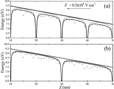
the applied and coulombic fields can be interpreted as a spatial deformation of the mobility edge above localized states, as illustrated for electrons in figure 1 for λ = 1 nm, Q = +e, F = 0.5×106 _V.cm-1_,

εr = 4, Rc = 10 and 20 nm. The thick line is the mobility edge in absence of neutralization of distant

centres, i.e. when all coulombic centres contribute to the electron potential energy, whereas the dashed line corresponds to a localized electron which only feels the potential of the nearest charged centre. The difference between these two situations is quite negligible for Rc = 20 nm and remains slight for

Rc = 10 nm, that is for a high concentration of coulombic centres (about 1018 cm-3). Even if

neutralization of distant ions is not explicitly included in calculations, hopping rates between localized states are therefore mainly perturbed by the first – and at worst the second – neighbouring defect, and not by more distant ions.

3. Small polaron hopping motion

In the small polaron problem, charge carriers get localized because they dig their own potential well by distorting the surrounding medium. The non-occupied sites can be regarded as zero energy centres (ε = 0), whereas the filled site can be characterized by the polaron activation energy ε = Δ. Then, the intrinsic energy difference between the sites involved in a jump is constant, Δik = Δ, and hops

essentially take place between first neighbours.

10 20 30 40 50 6.0 6.5 7.0 7.5 8.0 8.5 9.0 9.5 10.0 10 20 30 40 50 6.0 6.5 7.0 7.5 8.0 8.5 9.0 9.5 10.0 F = 0.5x106 V cm-1 En er gy ( eV )

(a)

(b)

E nergy ( eV ) Z (nm)

Figure 1. Mobility edge given by the electron potential energy against position for (a) Rc = 10 nm,

(b) Rc = 20 nm, in absence of coulombic centres (straight line), by including the contribution of all

ions (thick solid line) and by considering the nearest charged centre only (dashed lines). The dots represent a statistical distribution of localized states below the mobility edge.

Since the field-lowering of the small polaron activation energy is only one half of the difference in the site potential energies [4], the q(Vi – Vk) term in (3) has to be replaced by q(Vi – Vk)/2. In absence

of coulombic potential wells, the simulation of the polaron hopping motion leads to the same mobility as (1) at low fields, with:

( )

∝

(

− _d

)

⎜_⎝⎛ Δ− _{k T}⎟_⎠⎞ T k e µ B B exp 2 exp 0 2 λ λ . (7)

This result is normal since both the analytical theory and the simulation make use of one-dimensional models based on similar hopping rates [4,5]. At high fields, the computed mobility departs from (1) and takes the decreasing form:

( )

(

)

F d R F µ λ λ_exp 2 0 − = . (8)

This law is satisfied when the field magnitude F exceeds the critical value F0 = 2Δ/eλ. Then, the condition q(Vi – Vk)/2 > Δ is always satisfied and the simulation mostly generates forward jumps at a

rate R = R0exp(-2λ/d). Correspondingly, the effective velocity of hopping carriers becomes constant, equal to Rλ, and the mobility obeys expression (8). This simplistic behaviour is inherent in the simulation model; the high field mobility derived by Emin [5] is most probably more physical.

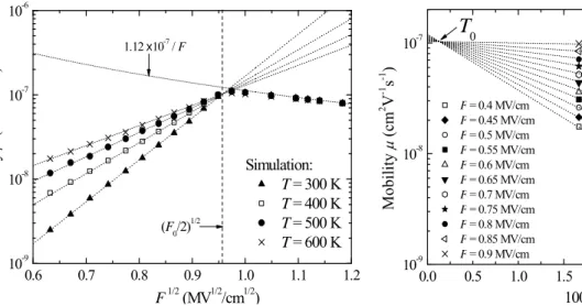
Coulombic potential wells strongly affect the field and temperature dependence of the mobility as illustrated in figures 2 and 3. The data have been obtained from simulations carried out with Q = +e (carriers are electrons), εr = 4, Rc = 10 nm, R0 = 1012 s-1, λ = 2 nm, d = 0.5 nm, and Δ = 0.185 eV. The plots of figure 2 still exhibit two regimes with respect to the applied field. The high field decrease has to be connected to the behaviour discussed above. Because of the potential wells, the electrons can feel electric fields which locally exceed F and experience energy variations greater than eFλ, even for the shortest jumps. Thus, the high field decrease now begins below F0 = 2Δ/eλ (F01/2 = 1.36 MV1/2 cm-1/2

here). In the low field region, the plots are linear and the slopes depend on temperature. The straight lines intersect for a particular field which is found to be about F0/2 here. This indicates the mobility no longer depends on temperature when the applied field is Δ/eλ. As shown in figure 3, the temperature dependence of the mobility has similar properties: the plots are straight lines which intersect for a particular value T0 (the mobility is therefore independent of the field when T = T0).

0.6 0.7 0.8 0.9 1.0 1.1 1.2 10-9 10-8 10-7 10-6 (F₀/2)1/2 1.12 x10-7 / F Simulation: T = 300 K T = 400 K T = 500 K T = 600 K M obilit y μ (cm 2 V -1 s -1 ) F1/2 (MV1/2/cm1/2) 0.0 0.5 1.0 1.5 2.0 2.5 3.0 3.5 10-9 10-8 10-7 Mobi li ty μ (c m 2 V -1 s -1 ) F = 0.4 MV/cm F = 0.45 MV/cm F = 0.5 MV/cm F = 0.55 MV/cm F = 0.6 MV/cm F = 0.65 MV/cm F = 0.7 MV/cm F = 0.75 MV/cm F = 0.8 MV/cm F = 0.85 MV/cm F = 0.9 MV/cm 1000/T (K-1)

T

₀

Figure 2. Mobility against the square-root of the electric field at different temperatures and fits of the low-field data with equation (1) (dashed lines).

Figure 3. Mobility against the temperature at low field and fits with equation (1) (dashed lines). The preceding features demonstrate that the simulation reproduces the phenomenological mobility (2) proposed by Gill [17] for F ≤ Δ/eλ (low fields). The fit of the simulation results with this expression allows an estimate of the relevant parameters:

µ0 = 10-7 cm2 V-1 s-1 ; E0 = 0.295 eV ; β = 0.308 eV MV-1/2 cm1/2 ; T0 ≈ 7500 K

The corresponding plots are drawn in dashed lines in figures 2 and 3. The β value is rather close to the Poole-Frenkel coefficient βPF = e(Q/πε0εr)1/2 for Q = +e and εr = 4, i.e. βPF = 0.379 eV MV-1/2 cm1/2 if ε0 = 8.85×10-12 F m-1. A better agreement was found from other calculations where each coulombic well extend over (‘contains’) more localized states, that is with Rc = 20 nm (β = 0.342, E0 = 0.32 eV) or λ = 1 nm (β = 0.381, E0 = 0.48 eV). In addition, fits of simulation data carried out for Rc = 10 nm, λ = 2 nm but Q = 2e lead to β = 0.558 (and E0 = 0.523 eV) while the Poole-Frenkel coefficient is 0.536 in this case. General behaviours shown in figures 2 and 3 have been found to be remarkably reproducible for all sets of investigated parameters. The Poole-Frenkel behaviour, i.e. proportionality between the logarithm of the mobility and the square-root of the field, is not the result of a presupposed mechanism. It is produced in a natural way due to the perturbations introduced by the coulombic wells in the carrier hopping rates.

Since the mobility is temperature independent when F≈Δ/eλ, the macroscopic activation energy E0 necessarily satisfies:

λ β

e

E0 ≈ Δ . (9)

This expression is only deduced from numerical calculations and is not derived from physical or even mathematical arguments. It is roughly verified for all sets of reported parameters (Q, Rc, λ and Δ have

been varied) within the error inherent in the simulation and fitting procedures. Perhaps a three dimensional simulation would lead to a slightly different relation, but one can nevertheless retain that the effective activation energy appearing at the scale of experiments is no longer the microscopic energy Δ as in equation (7). It now depends on Δ, but also on the mean distance λ between hopping sites and on the ion charge Q. This has a profound effect upon interpretation of experimental results since E0 cannot be uniquely associated with a trap depth or a polaron binding energy

.

4. Hopping in bandtails of disordered materials

We now consider hopping in site-ordered exponential bandtails [12-15]. The simulation differs from the small polaron study in the energy distribution of hopping sites. In order to reproduce the exponential density of localized states, proportional to exp(-ε/εc), an energy level εi is assigned to each

localization site by drawing a random number γi uniformly distributed between 0 and 1 such that εi = - εc ln(1 - γi). In one dimension, this procedure has to be repeated before each particle injection to

ensure the statistical reliability of the simulation. Hops are controlled by the competition between the spatial separation rik and the energy difference Δik = εi – εk between sites. A carrier can now jump to a

distant site whose energy is close to the occupied level instead of tunnelling to a neighbouring site. As expected, the simulation shows that hopping transport in an exponential bandtail is highly dispersive. It is therefore convenient to present the results in terms of transient current I(t) and transit-time tT. I(t) is calculated from the knowledge of the instant amount NS of carriers contained in the

sample and from the evaluation of their mean position Z . To make the results independent of the number Ntot of simulated particles, I(t) is expressed in the reduced form (10) with the dimension of an

inverse time (s-1_):

( )

dt Z d N N L t I tot s simul 1 = . (10)

The bandtail width has been fixed by setting εc = 0.0862 eV. Although arbitrary, this choice makes the low field dispersion parameter α = kBT/εc easy to calculate (one then has α = T/1000). The calculations also use the following parameters: R0 = 1012 s-1, λ = 1 nm, d = 0.5 nm, L = 200 nm.

In absence of coulombic wells, the computed current reproduces the properties pointed out by prior researches [12-15]. It is governed by an intricate interplay between temperature and field effects. For sufficiently low temperature and applied fields, the current satisfies the power law time dependence predicted by Scher and Montroll [3], where A and B are constants:

( )

₍( ₎) ⎪⎩ ⎪ ⎨ ⎧ > < = ₋− ₊− T T t t Bt t t At t I _α α 1 1 . (11)

The dispersion parameter is well given by α = kBT/εc at low field but it becomes field-dependent as the field is increased. This feature is illustrated on figure 4 by the simulated currents obtained for

T = 600 K (kBT < εc) and several applied field (F = 0.1, 0.3 and 0.6×106 V cm-1). For the lowest F value, the data are well fitted by (11) with α = 0.6, as expected from α = T/1000. For F = 0.3 and 0.6×106 _{V cm}-1_{, one has α = 0.62 and 0.69 respectively. Transit-times can be estimated from the fitted} plots according to tT = (B/A)1/2α. The values calculated for a significant set of temperatures indicate

that the transit time is thermally activated: tT ∝ exp(Ea/kBT). A reproducible activation energy Ea about 0.2 eV was found for all the considered field.

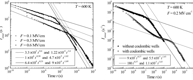
10-10 10-9 10-8 10-7 10-6 10-5 104 105 106 107 108 3.3 x103 t-0,4 and 1.22 x10-4 t-1,6 1 x104 t-0,38 and 4.7 x10-5 t-1,62 6.4 x104 t-0,31 and 9 x10-6 t-1,69 T = 600 K F = 0.1 MV/cm F = 0.3 MV/cm F = 0.6 MV/cm Isim u l (s -1 ) Time t (s) 10 -10 10-9 10-8 10-7 10-6 10-5 10-4 10-3 10-2 101 102 103 104 105 106 107 108 Time t (s) Isimu l (s -1 ) 9 x103 t-0,37 and 5.5 x10-5 t-1,63 180 t-0,37 and 1.1 x10-3 t-1,63

without coulombic wells with coulombic wells

T = 600 K

F = 0.2 MV cm-1

at T = 600 K. The fits by the power-law functions are shown. For each plot, the transit time is given by the intersection of the two straight-lines.

at T = 600 K and F = 0.2×106 _{V cm}-1 _{in absence} and in presence of coulombic defects. The fits show that the dispersion parameter is not modified. Changes induced by the presence of the coulombic potentials are illustrated in figure 5 for Q = +e,

Rc = 10 nm, T = 600 K and F = 0.2×106 V cm-1. The coulombic wells slow-down the carrier motion

and are responsible for a decrease in the instantaneous current as well as for an increase in the transit time. However, the current still obeys the power-law approximation (11) around the transit time for the same dispersion parameter α = 0.63 as for intrinsic transport (the ionized defects do not affect

dispersion). Calculations carried out at other T (500 K, 700 K) and F (0.3, 0.4×106 _{V cm}-1_{) confirmed} that α is independent of the presence of charged defects.

Equation (11) does not provide a proper description of the current at short time because of the delay required to reach the steady-state regime of trap-limited transport. The regions where the current decay follows straight lines are therefore ‘shortened’ and this affects the accuracy of the estimate of coefficients involved in (11). Even if any small change in A or B (or also α) only leads to a small shift of the transit time location on the logarithmic scale, it yields a significant change in the corresponding value. The evaluation of the trap-modulated transit-times t’T has been carried out for a set of applied

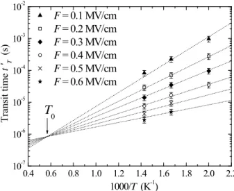
fields and temperatures. In each case, the extreme straight lines (upper and lower limits) which could reasonably fit the data on both sides of the transit time were considered. We then deduced a corresponding transit time range and noticed that the discrepancies never exceed a 20% relative error. The plots of figures 6 and 7 show the values of t’T taken at the middle of the error range, as a function

of F1/2 _{and 1000/T respectively, together with the error bars accounting for the overall 20%} uncertainty. Note that two points are not reported for the lowest temperature and the highest fields considered here, that is at T = 500 K, F = 0.5 and 0.6 MV cm-1_{. In these cases, field effects prevail} over thermal ones and the steady-state trap-limited transport is not established before the first carrier transit. As a consequence, the related currents plots depart markedly from straight lines and the transit times can not be calculated in the framework of equation (11). Within the admitted error, impurity-limited transit times follow straight-lines which intersect for a particular field Fc and temperature T0. They therefore satisfy:

(

)

⎥ ⎥ ⎦ ⎤ ⎢ ⎢ ⎣ ⎡ ⎟⎟ ⎠ ⎞ ⎜⎜ ⎝ ⎛ − − ′ = ′ 0 0 0 1 1 exp , T T k F E t T F t B T T β . (12)

The fits shown in dashed lines have been obtained for the following parameters:

t’T0 = 8.4×10-7 s ; E0 = 0.64 eV ; β = 0.645 eV MV-1/2 cm1/2 ; T0 ≈ 1760 K

There is now an appreciable difference between the β coefficient and the expected Poole-Frenkel one (βPF = 0.379 eV MV-1/2 cm1/2). This discrepancy is not surprising with regard to the combined error introduced by the successive fits, but it prevents from any definitive conclusion. The apparent activation energy E0,related to the critical field Fc by E0 = βFc1/2, differs from the mean energy εc of the bandtail states and is greater than the 0.2 eV energy obtained in absence of coulombic defects.

0.2 0.4 0.6 0.8 1.0 1.2 10-7 10-6 10-5 10-4 10-3 10-2

T = 500 K

T = 600 K

T = 700 K

F

_c Transit time t ' T (s ) F1/2 (MV1/2/cm1/2) 0.4 0.6 0.8 1.0 1.2 1.4 1.6 1.8 2.0 2.2 10-7 10-6 10-5 10-4 10-3 10-2 T ransit time t 'T (s) F = 0.1 MV/cm F = 0.2 MV/cm F = 0.3 MV/cm F = 0.4 MV/cm F = 0.5 MV/cm F = 0.6 MV/cm

T

₀ 1000/T (K-1)

Figure 6. Transit-time against the square-root of the electric field at different temperatures and fits of the low-field data with the inverse of equation (1) (dashed lines).

Figure 7. Transit-time against 1000/T at different

fields and fits of the low-field data with the inverse of equation (1) (dashed lines).

5. Discussion

It has been demonstrated in sections 3 and 4 that, statistically, the average mobility and transit time produced by the hopping rate (3) exhibit a Poole-Frenkel-like field dependence and a modified Arrhenius behaviour characterized by a critical temperature T0. Two questions are then remaining: is the β coefficient of the phenomenological mobility (2) really the same as the Poole-Frenkel one and why? What is the physical origin of T0 and what are the parameters which control its value?

The well-known Poole-Frenkel (PF) model basically describes the classical emission of a carrier from a energy depth Et at the centre of a coulombic or neutral trap over a barrier lowered by a uniform external field [21,22]. If an external field of magnitude F is turned towards the – x direction, the potential energy of a carrier q at a distance x from a coulombic centre can be written as:

( )

qFx q x x E = + 4 2 PF p β . (13)

The constant βPF is defined as in section 3, that is here βPF = |q|(Q/πε0εr)1/2, so βPF2/4|x|q2 is the coulombic potential (6) in one dimension. The maximum of potential energy occurs at

x0 = βPF /2|q|F1/2, where Ep = sign(q) βPF F1/2. Then, if the coulombic contribution in (13) and the trap

depth Et are measured with respect to the potential energy at infinity, a trapped carrier will be emitted if it passes over a barrier Et - βPF F1/2 and the thermal emission rate W from the coulombic trap is:

⎟ ⎟ ⎠ ⎞ ⎜ ⎜ ⎝ ⎛ − × = T k F E W W B PF t 0 exp β . (14)

Corrections to this simple theory generally result in multiplying the barrier lowering by a correction factor [22].

Let us now turn to the case of hopping transport. For the sake of simplicity, we focus here on the small polarons hopping motion for which the most probable hops take place between nearest neighbours (the hopping range is just λ, the mean distance between sites). If one assumes positive xi, the potential energy variation accompanying a hop from site i to site k is given by equations (15) and (16) for forward and backward jumps respectively.

(

)

₍

₎

_⎥ ⎦ ⎤ ⎢ ⎣ ⎡ − + = − 1 2 0 λ λ i i k i x x x qF V V q , xk = xi + λ, (15)

(

)

₍

₎

_⎥ ⎦ ⎤ ⎢ ⎣ ⎡ − − = − λ λ i i k i x x x qF V V q 2 0 1 , xk = xi – λ. (16)

If the centres are positively charged and carriers are electrons (Q > 0, q <0), a forward jump in space will correspond to a upward hop in energy if q(Vi – Vk) < 0 in (15), that is if xi is smaller than the

critical value xc defined as:

⎟ ⎟ ⎠ ⎞ ⎜ ⎜ ⎝ ⎛ − ⎟ ⎠ ⎞ ⎜ ⎝ ⎛ + = 1 4 1 2 2 0 c _λ λ x x . (17)

Similarly, (16) indicates that a backward jump in space will always correspond to a downward hop in energy if xi is smaller than xc + λ. As a consequence, carriers located on a site between 0 and xc mainly undergo backward hops, i.e. towards the centre, and are likely to remain below xc: they are “trapped”. For carriers located on a site beyond xc + λ, forward jumps correspond to downward hops whereas backward jumps are upward hops in energy. Thus, a carrier that has moved beyond xc + λ is likely to move away from the centre: it is emitted. For carriers between xc and xc + λ, both forward and backward jumps will produce downward hops in energy, but the backward jump will favour trapping while the forward jump will favour emission. The hop direction then depends on F, Q and λ. For instance, if λ or Q are such that q(Vi – Vk) exceeds the polaron activation energy, equations (3)-(5) will make the probability of emission greater than that of capture.

A carrier bound to a coulombic centre requires a certain average energy Ea to escape from the centre, just as in the classical PF effect, but this energy does not now refer to the edge of the barrier at

x0 (edge of the conduction band), but to some level between xc and xc + λ at which the probability to escape is sufficiently high. One has:

a 0 a

a E E

E = −Δ , (18)

where Ea0 is the average energy of electrons “trapped” below xc at equilibrium and ΔEa is the barrier lowering now given by the potential energy at xc. Note that xc and xc + λ both tends to x0 when λ tends to zero, so the classical PF effect is then recovered (continuous distribution of states along the band edge). In normal conditions, when the coulombic trap contains a significant numbers of localized sites between x = 0 and x = xc (x0/λ << 1), one has:

⎟⎟ ⎠ ⎞ ⎜⎜ ⎝ ⎛ − − = 0 0 c 4 1 2 x x x λ λ . (19)

Therefore, xc is slightly smaller than x0. Correspondingly the barrier lowering at xc, given by equation (20), is slightly greater than for the classical PF.

⎟ ⎟ ⎠ ⎞ ⎜ ⎜ ⎝ ⎛ ⎟⎟ ⎠ ⎞ ⎜⎜ ⎝ ⎛ + = Δ 2 0 PF a 8 1 1 x F E β λ . (20)

This result suggests that the barrier lowering is not exactly the same in case of hopping transport as in the classical effect. The difference is not constant when the applied field varies (it decreases at low fields due to the increase of x0), so the correction factor between βPF and the constant coefficient β in (2) probably correspond to a mean correction averaged over the experimental field range. With regard to the experimental and fitting errors, one can reasonably retain that both coefficients are roughly the same. As regards our simulations, it is also difficult to discriminate between physical corrections and statistical and fitting errors in the deviations between βPF and β. However, it has been mentioned in section 3 that increasing the number of centres within the coulombic radius, i.e. decreasing λ/x0 at all fields, well produces a β value much closer to the expected one βPF: the β value was found to be 0.381for λ =1 nm instead of 0.308 with λ = 2 nm, while the theoretical βPF value is 0.379.

The T0 values reported in sections 2 and 4 are high, from about 1700 K for dispersive hopping transport up to 7500 K for small polaron motion. If experimental values of T0 in the range 550 – 660 K

have been reported for electrons and holes by Gill in TNF:PVK [17], the theoretical model of Rackovsky and Scher [18] predicts values between about 500 K and almost infinity. Our T0 values are of course included in this infinitely broad range, but comparison is difficult because of the differences in treatment: the T0 values in [18] are shown to depend on the initial position of the carrier on the lattice with respect to the coulombic centre while this position is not retained as a parameter in our study. It is likely that simulations based on equation (3) would have yielded different T0 values if the injection site (Z = 0 here, see section 1) has been varied. Actually, making an attempt at finding a straightforward interpretation of T0, based on first principles and simple arguments, proves to be a very hard task. One may say that the modified Arrhenius behaviour is certainly associated with the field-assisted trapping of carriers since the derivative of the mobility (2) becomes a decreasing function of the field when T > T0 [18]. This idea is consistent with the dependence of T0 on the initial site because the latter also affects the trapping probability. To stand comparison with the experimentally measured

T0, which are of course independent of the initial position, the study would require a detailed calculation of the trapping and release probabilities averaged over a large number of initial sites. In this respect it seems that neither the present simulations nor the Rackovsky and Scher’s model are suitable for a proper examination of the modified Arrhenius law and of T0.

6. Conclusion

The phenomenological mobility (2), first reported by Gill [17] for dispersive transport, was related to hopping in presence of coulombic traps long time ago [19]. A formal derivation was given quite recently by Rackovsky and Scher, but with a substantial formalism and in the context of gaussian transport only [18]. The present work demonstrates that this mobility is actually consistent with the simplest model of hopping motion in presence of coulombic potential wells at low field. It also extends the conclusion of [18] by showing that the basic characteristics of this mobility, namely the Poole-Frenkel field dependence and the modified Arrhenius behaviour, are not only obtained for the gaussian motion of polarons, but also in case of an highly dispersive intrinsic transport (hopping in bandtails of disordered materials) provided the mobility is estimated after µ ∝ 1/t’T as in the Gill’s

experiments.

Trap-limited mobilities also exhibit a Poole-Frenkel field dependence in the multiple-trapping (MT) model of gaussian transport (see [23,24] for recent treatments of MT for gaussian and dispersive transport). In this situation however, the field-assisted lowering of the activation energy is initially assumed and included in the thermal release frequency W from coulombic traps (equation (14)). It finally comes out in the apparent steady-state mobility because the latter is simply given by µ = τW for

sufficiently deep traps, where τ is the mean lifetime before trapping. Then, the apparent activation energy of µ is necessarily the same as the microscopic trap energy Et in W. As regards hopping, the Poole-Frenkel behaviour appears naturally, i.e. without underlying assumption, because hopping rates are perturbed by the coulombic potential. In this respect, hopping transport is rather limited by the electrical perturbation due to defects than by trapping on a band-gap level in the MT sense. Then, the apparent activation energy E0 in (2) is not simply related to a trap depth or to energies characterizing intrinsic transport. It depends on the extrinsic limiting defects through the coefficient β, comparable to the Poole-Frenkel coefficient, and is therefore proportional to the square-root of the defect charge Q1/2_. It also depends on the critical field F0 where the mobility (2) is temperature independent and so probably on the mean distance between localized states.

Properties of anomalous dispersive transport resulting from MT on an exponential trap distribution are also similar to that of hopping in an exponential bandtail. Both mechanisms give rise to currents obeying equation (11) with the same dispersion parameter α = kBT/εc [2,23,24]. Discrepancies between these models are expected at short time and high field. First, high field hopping transport is characterized by a field-dependent dispersion parameter which departs from the low field value. Second, multiple-trapping can yield a specific current behaviour at short time [23,24]. In all cases, discrimination between coulombic trap-limited MT and hopping can be done because of the modified Arrhenius law characterizing hopping, provided the effective temperature (1/T –1/T0)-1 clearly differs from T. The crossing temperatures T0 reported in figures 3 and 7 are very high and confusion would be possible at low T in the situation of an experimental data analysis. A detailed study of the origin and of the dependence of T0 and F0 or Fc is beyond the scope of this paper whose objective is mostly a qualitative demonstration of basic properties.

References

[1] Blaise G 2001 J. Electrostat 50 69-89

[2] Pfister G and Scher H 1978 Adv. Phys. 27 747-798

[3] Scher H and Montroll E W 1975 Phys. Rev. B 12 2455-2477 [4] Austin I G and Mott N F 1969 Adv. Phys. 18 41-102

[5] Emin D 1975 Adv. Phys. 24 305-348 [6] Emin D 1991 Phys. Rev. B 43 11720-11724

[7] Scher H and Lax M 1973 Phys. Rev. B 7 4491-4502 [8] Scher H and Lax M 1973 Phys. Rev. B 7 4502-4519

[9] Arkhipov V I, Heremans P, Emelianova E V, Adriaenssens G J and Bässler H 2002 J. Phys.:

Condens. Matter 14 9899-9911

[10] Arkhipov V I, Heremans P, Emelianova E V, Adriaenssens G J and Bässler H 2003 Chem. Phys. 288 51-55

[11] Arkhipov V I, Heremans P, Emelianova E V, Adriaenssens G J and Bässler H 2004 J.

Non-Cryst. Solids 338-340 603-606

[12] Marianer S and Shklovskii B I 1992 Phys. Rev. B 46 13100-13103

[13] Cleve B, Hartenstein B, Baranovskii S D, Scheidler M, Thomas P and Baessler H 1995 Phys.

Rev. B 51 16705-16713

[14] Silver M, Schoenherr G and Baessler H 1982 Phys. Rev. Lett. 48 352-355

[15] Devlen R I, Antoniadis H, Schiff E A and Tauc J 1993 Philos. Mag. B 68 341-355 [16] Grünewald M, Movaghar B, Pohlmann B and Würtz D 1985 Phys. Rev. B 32 8191-8196 [17] Gill W D 1972 J. Appl. Phys. 43 5033-5040

[18] Rackovsky S and Scher H 1999 J. Chem. Phys. 111 3668-3674 [19] Jonscher A K and Ansari A A 1971 Philos. Mag. 23 205-223 [20] Miller A and Abrahams E 1960 Phys. Rev. 120 745-755 [21] Arnett P C and Klein N 1975 J. Appl. Phys. 46 1399-1400

[22] Martin P A, Streetman B G and Hess K 1981 J. Appl. Phys. 52 7409-7415

[23] Mady F, Renoud R, Ganachaud J P and Bigarré J 2005 Phys. Stat. Sol. (b) 242 2089-2106 [24] Mady F, Reboul J M and Renoud R 2005 J. Phys. D: Appl. Phys. 38 2271-2275