HAL Id: hal-01570035
https://hal.inria.fr/hal-01570035
Submitted on 28 Jul 2017
HAL is a multi-disciplinary open access archive for the deposit and dissemination of sci-entific research documents, whether they are pub-lished or not. The documents may come from teaching and research institutions in France or abroad, or from public or private research centers.
L’archive ouverte pluridisciplinaire HAL, est destinée au dépôt et à la diffusion de documents scientifiques de niveau recherche, publiés ou non, émanant des établissements d’enseignement et de recherche français ou étrangers, des laboratoires publics ou privés.
Colouring graphs with constraints on connectivity
Pierre Aboulker, Nick Brettell, Frédéric Havet, Dániel Marx, Nicolas
Trotignon
To cite this version:
Pierre Aboulker, Nick Brettell, Frédéric Havet, Dániel Marx, Nicolas Trotignon. Colouring graphs with constraints on connectivity. Journal of Graph Theory, Wiley, 2017, 85 (4), pp.814-838. �10.1002/jgt.22109�. �hal-01570035�
Colouring graphs with constraints on connectivity
Pierre Aboulker1, Nick Brettell2, Fr´ed´eric Havet3, D´aniel Marx4, and Nicolas Trotignon2 1Universidad Andres Bello, Santiago, Chile
2CNRS, LIP, ENS de Lyon
3Project Coati, I3S (CNRS, UNS) and INRIA, Sophia Antipolis, France 4Institute for Computer Science and Control, Hungarian Academy of Sciences (MTA
SZTAKI)
October 10, 2016
Abstract
A graph G has maximal local edge-connectivity k if the maximum number of edge-disjoint paths between every pair of distinct vertices x and y is at most k. We prove Brooks-type theorems for k-connected graphs with maximal local edge-connectivity k, and for any graph with maximal local edge-connectivity 3. We also consider several related graph classes defined by constraints on connectivity. In particular, we show that there is a polynomial-time algo-rithm that, given a 3-connected graph G with maximal local connectivity 3, outputs an optimal colouring for G. On the other hand, we prove, for k ≥ 3, that k-colourability is NP-complete when restricted to minimally k-connected graphs, and 3-colourability is NP-complete when restricted to (k − 1)-connected graphs with maximal local connectivity k. Finally, we consider a parameterization of k-colourability based on the number of vertices of degree at least k + 1, and prove that, even when k is part of the input, the corresponding parameterized problem is FPT.
Keywords: colouring; local connectivity; local edge-connectivity; Brooks’ theorem; minimally k-connected; vertex degree.
1
Introduction
We consider the problem of finding a proper vertex k-colouring for a graph for which, loosely speaking, the “connectivity” is somehow constrained. For example, if we consider the class of
The first author was supported by Fondecyt Postdoctoral grant 3150314 of CONICYT Chile. The second, third, and fifth authors were partially supported by ANR project Stint under reference ANR-13-BS02-0007 oper-ated by the French National Research Agency (ANR). The second and fifth authors were partially supported by ANR project Heredia under reference ANR-10-JCJC-0204, and by the LABEX MILYON (ANR-10-LABX-0070) of Universit´e de Lyon, within the program “Investissements d’Avenir” (ANR-11-IDEX-0007) operated by the French National Research Agency (ANR). The fourth author was supported by the European Research Council (ERC) grant “PARAMTIGHT: Parameterized complexity and the search for tight complexity results,” reference 280152 and OTKA grant NK105645.
Email addresses: [email protected] (P. Aboulker), [email protected] (N. Brettell), [email protected] (F. Havet), [email protected] (D. Marx), [email protected] (N. Trotignon).
graphs of degree at most k, then, by Brooks’ theorem, it is easy to find if a graph in this class is k-colourable.
Theorem 1.1 (Brooks, 1941). Let G be a connected graph with maximum degree k. Then G is k-colourable if and only if G is not a complete graph or an odd cycle.
On the other hand, if we consider the class of graphs with maximum degree 4, then the deci-sion problem 3-colourability is well known to be NP-complete, even when restricted to planar graphs [9]. Moreover, for any fixed k ≥ 3, k-colourability is NP-complete.
The classes we consider are defined using the notion of local connectivity. The local connectivity κ(x, y) of distinct vertices x and y in a graph is the maximum number of internally vertex-disjoint paths between x and y. The local edge-connectivity λ(x, y) of distinct vertices x and y is the maximum number of edge-disjoint paths between x and y. Consider the following classes:
• Ck
0: graphs with maximum degree k,
• Ck
1: graphs such that λ(x, y) ≤ k for all pairs of distinct vertices x and y,
• Ck
2: graphs such that κ(x, y) ≤ k for all pairs of distinct vertices x and y, and
• Ck
3: graphs such that κ(x, y) ≤ k for all edges xy.
In each successive class, the connectivity constraint is relaxed; that is, C0k ⊆ Ck
1 ⊆ C2k ⊆ C3k. For
each class, there is a bound on the chromatic number; we give details shortly. Note also that each of the four classes is closed under taking subgraphs.
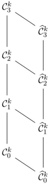
A graph G is k-connected if it has at least 2 vertices and κ(x, y) ≥ k for all distinct x, y ∈ V (G). The connectivity of a graph G is the maximum integer k such that G is k-connected. A graph contained in one of the above classes has connectivity at most k. So, for each class, it may be of interest to start by considering the graphs that have connectivity precisely k. For each class Cik, we denote by bCk
i the subclass containing the k-connected members of Cik. A Hasse diagram illustrating
the partial ordering of these classes under set inclusion is given in Figure 1.
A graph in C1k is said to have maximal local edge-connectivity k. Our first main result is a Brooks-type theorem for graphs with maximal local edge-connectivity k. An odd wheel is a graph obtained from a cycle of odd length by adding a vertex that is adjacent to every vertex of the cycle. Theorem 1.2. Let G be a k-connected graph with maximal local edge-connectivity k, for k ≥ 3. Then G is k-colourable if and only if G is not a complete graph or an odd wheel.
Note that an odd wheel is not 4-connected, so the condition that G is not an odd wheel is only required when k = 3.
Although every graph with maximum degree k has maximal local edge-connectivity k, Theo-rem 1.2 is not, strictly speaking, a generalisation of Brooks’ theoTheo-rem, since it only concerns such graphs that are k-connected. However, for k = 3 we prove an extension of Brooks’ theorem that characterises which graphs with maximal local edge-connectivity 3 are 3-colourable, with no re-quirement on 3-connectivity.
Let G1 and G2 be graphs and, for i ∈ {1, 2}, let (ui, vi) be an ordered pair of adjacent vertices
of Gi. We say that the Haj´os join of G1 and G2 with respect to (u1, v1) and (u2, v2) is the graph
obtained by deleting the edges u1v1 and u2v2from G1 and G2, respectively, identifying the vertices
u1 and u2, and adding a new edge joining v1 and v2. A block of a graph G is a maximal connected
Ck 3 b Ck 3 Ck 2 b Ck 2 Ck 1 b Ck 1 Ck 0 b Ck 0
Figure 1: Hasse diagram of the graph classes defined by constraints on connectivity under ⊆.
Theorem 1.3. Let G be a graph with maximal local edge-connectivity 3. Then G is 3-colourable if and only if each block of G cannot be obtained from an odd wheel by performing a (possibly empty) sequence of Haj´os joins with an odd wheel.
For convenience, we call a graph that can be obtained from an odd wheel by performing a sequence of Haj´os joins with odd wheels, a wheel morass. Suppose that G1 and G2 are wheel
morasses. It can be shown, by a routine induction argument, that the Haj´os join of G1 and G2 is
itself a wheel morass.
It follows from Theorems 1.2 and 1.3 that there is a polynomial-time algorithm that finds a k-colouring for a k-connected graph with maximal local edge-connectivity k, or determines that no such colouring exists; and there is a polynomial-time algorithm for finding an optimal colouring of any graph with maximal local edge-connectivity 3.
A graph in C2kis also said to have maximal local connectivity k. These graphs have been studied previously; primarily, the problem of determining bounds on the maximum number of possible edges in a graph with n vertices and maximal local connectivity k has received much attention (see [2, 14, 20, 23]). Note that for a k-connected graph G with maximal local connectivity k (that is, for G in bCk
2), we have κ(x, y) = k for all distinct x, y ∈ V (G). When k = 3, it turns out that
b C3
1 = bC23 (see Lemma 4.1). This leads to the following:
Theorem 1.4. Let G be a connected graph with maximal local connectivity 3. Then G is 3-colourable if and only if G is not an odd wheel. Moreover, there is a polynomial-time algorithm that finds an optimal colouring for G.
However, we give an example in Section 4 to demonstrate that bC4
1 6= bC24 (see Figure 5).
The class bCk
3 is well known. A graph G is minimally k-connected if it is k-connected and the
removal of any edge leads to a graph that is not k-connected. It is easy to check that a graph is in b
Ck
C3 3 b C3 3 (Proposition 1.6) C3 2 (Proposition 1.5) C3 1 (Theorem 1.3) b C3 1= bC23 (Theorem 1.4) C3 0 (Brooks’ Theorem) b C3 0 NP-hard P (a) k = 3 Ck 3 b Ck 3 (Proposition 1.6) Ck 2 b Ck 2 (Question 1.7) Ck 1 (Conjecture 1.8) b Ck 1 (Theorem 1.2) Ck 0 (Brooks’ Theorem) b Ck 0 NP-hard open P (b) k ≥ 4
Figure 2: k-colouring complexity for graph classes defined by constraints on connectivity. We now review known results regarding the bounds on the chromatic number of these classes. Mader proved that any graph with at least one edge contains a pair of adjacent vertices whose local connectivity is equal to the minimum of their degrees [21]. It follows that any graph in C3k has a vertex of degree at most k. This, in turn, implies that a graph in Ck
3 is (k + 1)-colourable.
In particular, minimally k-connected graphs, and graphs with maximal local connectivity k, are all (k + 1)-colourable.
Despite these results, it seems that, so far, the tractability of computing the chromatic number, or finding a k-colouring, for a graph in one of these classes has not been investigated. For fixed k, let k-colouring be the search problem that, given a graph G, finds a k-colouring for G, or determines that none exists. An overview of our findings in this paper is given in Figure 2, where we illustrate the complexity of k-colouring when restricted to the various classes defined by constraints on connectivity.
If k = 1, then Ck
3 is the class of forests, so all the classes are trivial. For k = 2, since it is easy
to determine if a graph is 2-colourable, and all graphs in C3k are 3-colourable, we may compute the chromatic number of any graph in C3k in polynomial time.
When k = 3, Theorem 1.4 implies that 3-colouring is polynomial-time solvable when re-stricted to bC3
2. For the class C13, this problem remains polynomial-time solvable, by Theorem 1.3.
One might hope to generalise these results in one of two other possible directions: to the class C23, or to bC3
3. But any such attempt is likely to fail, due to the following results (see Sections 4 and 5
respectively):
Proposition 1.5. For fixed k ≥ 3, the problem of deciding if a (k−1)-connected graph with maximal local connectivity k is 3-colourable is NP-complete.
Proposition 1.6. For fixed k ≥ 3, the problem of deciding if a minimally k-connected graph is k-colourable is NP-complete.
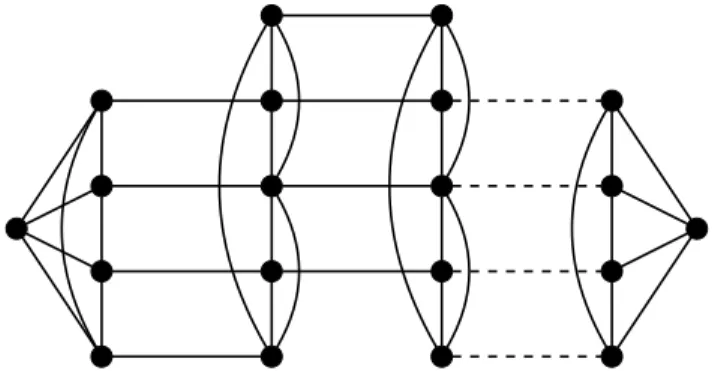
Figure 3: A 4-connected graph with maximal local edge-connectivity 4, and arbitrarily many vertices of degree more than 4.
solvable when restricted to bCk
1. However, the complexity for the more general class bC2k remains an
interesting open problem:
Question 1.7. For fixed k ≥ 4, is there a polynomial-time algorithm that, given a k-connected graph G with maximal local connectivity k, finds a k-colouring of G, or determines that none exists? We also show that 3-colourability is NP-complete for a graph in Ck
1, when k ≥ 4, so computing
the chromatic number for a graph in this class, or in Ck2, is NP-hard, as is 3-colouring. However, the complexity of k-colouring (or k-colourability) for these classes is unresolved. We make the following conjecture:
Conjecture 1.8. For fixed k ≥ 4, there is a polynomial-time algorithm that, given a graph G with maximal local edge-connectivity k, finds a k-colouring of G, or determines that none exists.
It is worth noting that the class bCk
1 is non-trivial. All k-connected k-regular graphs are members
of the class, as are k-connected graphs with n − 1 vertices of degree k and a single vertex of degree more than k. A member of the class can have arbitrarily many vertices of degree at least k + 1. To see this for k = 3, consider a graph G03,x, for x ≥ 3, that is obtained from a grid graph G3,x (the
Cartesian product of path graphs on 3 and x vertices) by adding two vertex-disjoint edges linking vertices of degree 2 at distance 2. The graph G03,x is in bC3
1, and has x − 2 vertices of degree 4. A
similar example can be constructed for any k > 3; for example, see Figure 3 for when k = 4. Finally, we consider a parameterization of k-colouring based on the number pkof vertices of
degree at least k + 1. By Brooks’ theorem, a graph G for which pk(G) = 0 can be k-coloured in
polynomial time, unless it is a complete graph or an odd cycle. We extend this to larger values of pk,
showing that, even when k is part of the input, finding a k-colouring for a graph is fixed-parameter tractable (FPT) when parameterized by pk.
Theorem 1.9. Let G be a graph with at most p vertices of degree more than k. There is a min{kp, pp} · O(n + m)-time algorithm for k-colouring G, or determining no such colouring exists. This paper is structured as follows. In the next section, we give preliminary definitions. In Section 3, we consider graphs with maximal local edge-connectivity k, and prove Theorems 1.2 and 1.3. We then consider the more general class of graphs with maximal local connectivity k, in Section 4, and prove Theorem 1.4 and Proposition 1.5. We present the proof of Proposition 1.6 in Section 5. Finally, in Section 6, we consider the problem of k-colouring a graph parameterized by the number of vertices of degree at least k + 1, and prove Theorem 1.9.
2
Preliminaries
Our terminology and notation follows [3] unless otherwise specified. Throughout, we assume all graphs are simple. We say that paths are internally disjoint if they have no internal vertices in common. A k-edge cut is a k-element set S ⊆ E(G) for which G\S is disconnected. A k-vertex cut is a k-element subset Z ⊆ V (G) for which G − Z is disconnected. We call the vertex of a 1-vertex cut a cut-vertex. For distinct non-adjacent vertices x and y, and Z ⊆ V (G) \ {x, y}, we say that Z separates x and y when x and y belong to different components of G − Z. More generally, for disjoint, non-empty X, Y, Z ⊆ V (G), we say that Z separates X and Y if, for each x ∈ X and y ∈ Y , the vertices x and y are in different components of G − Z. We call a partition (X, Z, Y ) of V (G) a k-separation if |Z| ≤ k and Z separates X from Y . When G is k-connected and (X, Z, Y ) is a k-separation of G, we have that |Z| = k. By Menger’s theorem, if κ(x, y) = k for non-adjacent vertices x and y, then there is a k-vertex cut that separates x and y. If κ(x, y) = k ≥ 2 for adjacent vertices x and y, then there is a (k − 1)-vertex cut in G\xy that separates x and y. We use these freely in the proof of Lemma 4.1.
We view a proper k-colouring of a graph G as a function φ : V (G) → {1, 2, . . . , k} where for every uv ∈ E(G) we have φ(u) 6= φ(v). For X ⊆ V (G), we write φ(X) to denote the image of X under φ.
Given graphs G1 and G2, the graph with vertex set V (G1) ∪ V (G2) and edge set E(G1) ∪ E(G2)
is denoted G1∪ G2.
A diamond is a graph obtained by removing an edge from K4. We call the two degree-2 vertices
of a diamond D the pick vertices of D.
3
Graphs with maximal local edge-connectivity k
In this section we prove Theorems 1.2 and 1.3.
Lov´asz provided a short proof of Brooks’ theorem in [18]. The proof can easily be adapted to show that graphs with at most one vertex of degree more than k are often k-colourable. We make this precise in the next lemma; the proof is provided for completeness. A vertex is dominating if it is adjacent to every other vertex of the graph.
Lemma 3.1. Let G be a 3-connected graph with at most one vertex of degree more than k, for k ≥ 3, and no dominating vertices. Then G is k-colourable.
Proof. Let h be a vertex of G with maximum degree. Since G has no dominating vertices and is connected, there is a vertex y at distance two from h. Let z1 be a common neighbour of h
and y. Since G is 3-connected, G − {h, y} is connected. Let z1, z2, . . . , zn−2 be a search ordering of
G−{h, y} starting at z1; that is, an ordering of V (G−{h, y}) where each vertex zi, for 2 ≤ i ≤ n−2,
has a neighbour zj with j < i. We colour G as follows. Assign h and y the colour 1, say. We can
then (greedily) assign one of the k colours to each of zn−2, zn−3, . . . , z2 in turn, since at the time
one of these vertices is considered, it has at most k − 1 neighbours that have already been assigned colours. Finally, we can colour z1, since it has degree at most k, but at least two of its neighbours,
h and y, are the same colour.
Now we show that we can decompose a k-connected graph with maximal local edge-connectivity k into components each containing a single vertex of degree more than k.
Lemma 3.2. Let G be a k-connected graph with maximal local edge-connectivity k, for k ≥ 3, and at least two vertices of degree more than k. Then there exists a k-edge cut S such that one component of G\S contains precisely one vertex of degree more than k, and the edges of S are vertex disjoint.
Proof. We say that a set of vertices X1 ⊆ V (G) is good if |X1| ≤ n/2 and d(X1) = k, where d(X1)
is the number of edges with one end in X1 and the other end in V (G) \ X1. If two good sets X1
and X2 have non-empty intersection, then |X1∪ X2| < n, so d(X1∪ X2) ≥ k by k-connectivity. As
d(X1) + d(X2) ≥ d(X1∪ X2) + d(X1∩ X2) (see, for example, [3, Exercise 2.5.4(b)]), it follows that
d(X1 ∩ X2) = k. Thus, if a good set X1 meets a good set X2, then X1∩ X2 is also good. This
implies that if a vertex of degree more than k is in a good set, then there is unique minimal good set containing it. Since there is a k-edge cut between any two vertices, one of any two vertices is in a good set. Thus, all but at most one vertex of G is in a good set. Let X be a minimal good set containing at least one vertex of degree more than k. Suppose X contains distinct vertices x and y, each with degree more than k. Then there is k-edge cut separating them, so there is a good set containing exactly one of them. By taking the intersection of this good set with X, we obtain a good set that is a proper subset of X and contains at least one vertex of degree more than k; a contradiction. So X contains precisely one vertex of degree more than k. Now d(X) = k, since X is good, hence the k edges with one end in X and the other in E(G) − X give an edge cut S.
It remains to show that the edges of S are vertex disjoint. Set Y = V (G) \ X, and let XS
(respectively, YS) be the set of vertices of X (respectively, Y ) incident to an edge of S. Let |X| = q.
Since every vertex in X has degree at least k, and X contains some vertex of degree more than k, we have that Σv∈Xd(v) ≥ qk + 1. If q ≤ k, then, since each vertex in X has at most q − 1
neighbours in X, we have that Σv∈Xd(v) ≤ q(q − 1) + k ≤ k(q − 1) + k = qk; a contradiction. So
XS6= X and, similarly, YS 6= Y . Now, since G is k-connected, there are k internally disjoint paths
from any vertex in X \ XS to any vertex in Y \ YS. Each of these paths must contain a different
edge of S. Thus S satisfies the requirements of the lemma.
Next we show, loosely speaking, that if a graph G has a k-edge cut S where the edges in S have no vertices in common, then the problem of k-colouring G can essentially be reduced to finding k-colourings of the components of G\S; the only bad case is when the vertices incident to S are coloured all the same colour in one component, and all different colours in the other.
Lemma 3.3. Let G be a connected graph with a k-edge cut S, for k ≥ 3, such that the edges of S are vertex-disjoint, and G\S consists of two components G1 and G2. Let Vi be the set of vertices
in V (Gi) incident to an edge of S, for i ∈ {1, 2}.
(i) Then G is k-colourable if and only if there exists a k-colouring φ1 of G1 and a k-colouring φ2
of G2 such that {|φ1(V1)|, |φ2(V2)|} 6= {1, k}.
(ii) Moreover, if φ1 and φ2 are k-colourings of G1 and G2, respectively, for which
{|φ1(V1)|, |φ2(V2)|} 6= {1, k}, then there exists a permutation σ such that
φ(x) = (
φ1(x) for x ∈ V (G1),
σ(φ2(x)) for x ∈ V (G2)
Proof. First, we prove (ii), which implies that (i) holds in one direction. Let φ1 and φ2 be
k-colourings of G1 and G2, respectively, for which {|φ1(V1)|, |φ2(V2)|} 6= {1, k}. We will construct an
auxiliary graph H where the vertices are labelled by subsets of V1 or V2 in such a way that if we
can k-colour H, then there exists a permutation σ such that φ, as defined in the statement of the lemma, is a k-colouring of G.
Let (T1, T2, . . . , T|φ1(V1)|) be the partition of the vertices in V1 into colour classes with respect to
φ1and, likewise, let (W1, W2, . . . , W|φ2(V2)|) be the partition of V2 into colour classes with respect to
φ2. We construct a graph H consisting of |φ1(V1)|+|φ2(V2)| vertices: for each i ∈ {1, 2, . . . , |φ1(V1)|},
we have a vertex ti ∈ V (H) labelled by Ti, and, for each i ∈ {1, 2, . . . , |φ2(V2)|}, we have a vertex
wi ∈ V (H) labelled by Wi. Let T = {ti : 1 ≤ i ≤ |φ1(V1)|} and let W = {wi : 1 ≤ i ≤ |φ2(V2)|}.
Each t ∈ T (respectively, w ∈ W ) is adjacent to every vertex in T − {t} (respectively, W − {w}). Finally, for each edge v1v2 in S, we add an edge between the vertex t ∈ T labelled by the colour
class containing v1, and the vertex w ∈ W labelled by the colour class containing v2, omitting
parallel edges. Thus there are at most k edges between vertices in T and vertices in W .
Now we show that H is k-colourable. Consider a vertex t ∈ T . If it has x neighbours in W , then it represents a colour class consisting of at least x vertices of V1. So there are at most k − x
vertices in T − {t}, and hence t has degree at most x + (k − x). It follows, by Brooks’ theorem, that H is k-colourable unless it is a complete graph, as k ≥ 3. Moreover, if |V (H)| ≤ k, then H is k-colourable, so assume that |V (H)| > k. Then, without loss of generality, we may assume that |T | > k/2. Since there are at most k edges between vertices in T and vertices in W , and each vertex of T has the same number of neighbours in W , it follows that each vertex in T has a single neighbour in W . Since H is a complete graph, we have |W | = 1, and hence, recalling that |V (H)| > k, we have |T | = k. That is, |φ1(V1)| = k and |φ2(V2)| = 1; a contradiction.
Now H is colourable. By permuting the colours of a colouring of H, we can obtain a k-colouring ψ such that ψ|V1 = φ1. Then ψ|V2 induces a permutation σ of φ2, in the obvious way,
with the desired properties. This completes the proof of (ii).
Finally, we observe that when {|φ1(V1)|, |φ2(V2)|} = {1, k} for every k-colouring φ1 of G1 and
every k-colouring φ2 of G2, then G is not k-colourable. This completes the proof of (i).
Suppose that a graph G has a k-edge cut S that separates X from Y , where (X, Y ) is a partition of V (G). We fix the following notation for the remainder of this section. Let YS (respectively, XS)
be the subset of Y (respectively, X) consisting of vertices incident to an edge in S. Let GX
(respectively, GY) be the graph obtained from G[X ∪ YS] (respectively, G[Y ∪ XS]) by adding edges
so that YS (respectively, XS) is a clique.
Lemma 3.4. Let G be a k-connected graph, for k ≥ 3, with maximal local edge-connectivity k, and a k-edge cut S that separates X from Y , where (X, Y ) partitions V (G). Then GX is k-connected
and has maximal local edge-connectivity k.
Proof. First we show that GX has maximal local edge-connectivity k. The only vertices of degree
more than k in GX are in X. Suppose u and v are vertices in X of degree more than k. Clearly,
for each uv-path in GX[X] there is a corresponding uv-path in G[X]. We show that there are at
least as many edge-disjoint uv-paths that pass through an edge of S in G as there are in GX; it
follows that λGX(u, v) ≤ λG(u, v) ≤ k. Since S is a k-edge cut in GX, there are at most bk/2c
edge-disjoint paths in GX starting and ending at a vertex in XS. Let y be a vertex in Y . Since G is
k-connected, the Fan Lemma (see, for example, [3, Proposition 9.5]) implies that there are k paths from y to each member of XS that meet only in y. Hence, there are bk/2c edge-disjoint paths in
G[Y ∪ XS] starting and ending at a vertex in XS. Thus, we deduce that GX has maximal local
edge-connectivity k.
We now show that GX is k-connected, by demonstrating that κGX(u, v) ≥ k for all distinct
u, v ∈ V (GX). First, suppose that u, v ∈ X. Evidently, for each uv-path in G[X] there is a
corresponding uv-path in GX[X]. Moreover, each uv-path in G that traverses an edge of S traverses
two such edges xy and x0y0, say, where x, x0 ∈ XS and y, y0 ∈ YS. By replacing the x0y0-path in G
with the edge x0y0 in GX, we obtain a uv-path of GX. We deduce that κGX(u, v) ≥ κG(u, v) ≥ k
for any u, v ∈ X. Now suppose u, v ∈ YS. Then there are k − 1 internally disjoint uv-paths in
GX[YS]. Pick u0, v0 ∈ XS such that uu0 and vv0 are in S. Since GX[X] is connected, there is at
least one u0v0-path in GX[X], so there are k internally disjoint uv-paths in GX. Finally, let u ∈ X
and v ∈ YS. Since G is k-connected, the Fan Lemma implies that there are k paths from u to
each vertex of YS in G that meet only in u. Hence there are k such paths in GX. Since YS is a
clique in GX, there are k internally disjoint uv-paths in GX. Thus κGX(u, v) ≥ k for all distinct
u, v ∈ V (GX), as required.
Proposition 3.5. Let G be a k-connected graph, for k ≥ 3, with maximal local edge-connectivity k and at least two vertices of degree more than k. Then G is k-colourable.
Proof. The proof is by induction on the number of vertices of degree more than k. First we show that the proposition holds when G has precisely two vertices of degree more than k. Let x and y be distinct vertices of G with degree more than k. By Lemma 3.2, there is a k-edge cut S that separates X from Y , where x ∈ X, y ∈ Y , (X, Y ) is a partition of V (G), and X contains precisely one vertex of degree more than k. Consider the graph GX; this graph is 3-connected by Lemma 3.4,
and has no dominating vertices by definition. Hence, by Lemma 3.1, GX is k-colourable. Moreover,
in such a k-colouring, the vertices in YS are given k different colours, since they form a k-clique,
and hence the vertices in XS are not all the same colour. So GX[X] = G[X] is k-colourable in such
a way that the vertices in XS are not all the same colour. By symmetry, G[Y ] is k-colourable in
such a way that the vertices in YS are not all the same colour. It follows, by Lemma 3.3, that G is
k-colourable.
Now let G be a graph with p vertices of degree more than k, for p > 2. We assume that a k-connected graph with maximal local edge-connectivity k, and p − 1 vertices of degree more than k is k-colourable. By Lemma 3.2, there is a k-edge cut S that separates X from Y , where X contains precisely one vertex x of degree more than k, and (X, Y ) is a partition of V (G). The graph GY
is k-connected and has maximal local edge-connectivity k, by Lemma 3.4. Thus, by the induction assumption, GY is k-colourable. It follows that G[Y ] is k-colourable in such a way that the vertices
in YS are not all the same colour. The graph GX is 3-connected, by Lemma 3.4, so is k-colourable,
by Lemma 3.1. So G[X] is k-colourable in such a way that the vertices in XS are not all the same
colour. Thus, by Lemma 3.3, G is k-colourable. The proposition follows by induction.
Proof of Theorem 1.2. Clearly if G is a complete graph, then G is Kk+1 and is not k-colourable. If
G is an odd wheel, then, since G is not 4-connected, we have k = 3, and G is not 3-colourable. This proves one direction. Now suppose G is not k-colourable and has p vertices of degree more than k. Then p < 2, by Proposition 3.5. If p = 0, then G is a complete graph, by Brooks’ theorem (an odd cycle is not k-connected for any k ≥ 3). If p = 1, then G has a dominating vertex v, by Lemma 3.1. Since G − {v} is not (k − 1)-colourable, and G − {v} has maximum degree k − 1, it follows, by Brooks’ theorem, that G − {v} is a complete graph or an odd cycle. Thus G is a complete graph or an odd wheel.
Corollary 3.6. Let G be a k-connected graph with maximal local edge-connectivity k. There is a polynomial-time algorithm that finds a k-colouring for G when G is k-colourable, or a (k + 1)-colouring otherwise.
Proof. Suppose G has at most one vertex of degree more than k. If G has no dominating vertices, then the proof of Lemma 3.1 leads to an algorithm for k-colouring G. Otherwise, when G has a dominating vertex v, the problem reduces to finding a (k − 1)-colouring for G − {v}, where G − {v} has maximum degree k − 1. In either case, we have a linear-time algorithm for colouring G.
When G has at least two vertices x and y of degree more than k, we use the approach taken in the proof of Proposition 3.5. We can find a k-edge cut S that separates x and y in O(km) time, by an application of the Ford-Fulkerson algorithm. Without loss of generality, x is contained in a component of G\S with at most n/2 vertices. It follows, by the proof of Lemma 3.2, that with O(n) applications of the Ford-Fulkerson algorithm we can obtain an edge cut S0 such that x is the only vertex of degree more than k in one component X of G\S0. Thus we can find the desired k-edge cut S0 in O(knm) = O(nm) time. Let Y = V (G) \ X, and let GX and GY be as defined
just prior to Lemma 3.4. As GX is 3-connected by Lemma 3.4, and has no dominating vertices by
definition, we can find a k-colouring φX for GX in linear time by Lemma 3.1. To find a k-colouring
φY for GY, if one exists, we repeat this process recursively. Then, by Lemma 3.3, we can extend
φY to a k-colouring of G by finding a permutation for φX, which can be done in constant time.
When G has p vertices of degree more than k, this process takes O(pnm) time. Since p ≤ n, the algorithm runs in O(n2m) time.
An extension of Brooks’ theorem when k = 3
We now work towards proving Theorem 1.3. Recall that a wheel morass is either an odd wheel, or a graph that can be obtained from odd wheels by applying the Haj´os join. We restate the theorem here in terms of wheel morasses:
Theorem 3.7. Let G be a graph with maximal local edge-connectivity 3. Then G is 3-colourable if and only if each block of G is not a wheel morass.
Let us now establish some properties of wheel morasses. A graph G is k-critical if χ(G) = k and every proper subgraph H of G has χ(H) < k.
Proposition 3.8. Let G be a wheel morass. Then (i) G is 4-critical, and
(ii) for every two distinct vertices x and y, we have λ(x, y) ≥ 3.
Proof. (i) It is well known that the Haj´os join of two k-critical graphs is k-critical (see, for example, [3, Exercise 14.2.9]). Since the odd wheels are 4-critical, we immediately get, by induction, that every wheel morass is 4-critical.
(ii) We prove this by induction on the number of Haj´os joins. The result can easily be checked for odd wheels.
Assume now that G is the Haj´os join of G1 and G2 with respect to (u1, v1) and (u2, v2). Let
x and y be two vertices in G. If x ∈ V (G1) and y ∈ V (G1), then, by the induction hypothesis,
there are three edge-disjoint xy-paths in G1. If one them contains v1u1, then replace it by the
induction hypothesis). This results in three edge-disjoint xy-paths, so λG(x, y) ≥ 3. Likewise, if
x ∈ V (G2) and y ∈ V (G2), then λG(x, y) ≥ 3.
Assume now that x ∈ V (G1) and y ∈ V (G2). Let us prove the following:
Claim 3.8.1. In G1\u1v1, there are three edge-disjoint paths P1, P2 and P3 such that P1 and P2
are xu1-paths and P3 is an xv1-path.
Proof. By the induction hypothesis, there are three edge-disjoint xu1-paths R1, R2, R3 in G1. If
v1 ∈ V (R1) ∪ V (R2) ∪ V (R3), then we may assume, without loss of generality, that v1 ∈ V (R3) and
u1v1 ∈ E(R/ 1)∪E(R2). Hence R1, R2and the xv1-subpath of R3 are the desired paths. Now we may
assume that v1∈ V (R/ 1)∪V (R2)∪V (R3). Let Q be a shortest path from z1∈ V (R1)∪V (R2)∪V (R3)
to v1 in G\u1v1 (such a path exists by our connectivity assumption). Without loss of generality,
z1 ∈ V (R3). Hence the desired paths are R1, R2 and the concatenation of the xz1-subpath of R3
and Q. This proves Claim 3.8.1.
By Claim 3.8.1 and symmetry, there are three edge-disjoint paths Q1, Q2 and Q3 in G2\u2v2
such that Q1 and Q2 are u2y-paths and Q3 is a v2y-path. The paths obtained by concatenating P1
and Q1; P2 and Q2; and P3, v1v2 and Q3are three edge-disjoint xy-paths in G, so λG(x, y) ≥ 3.
Proof of Theorem 1.3. If a block of G is a wheel morass, then this block has chromatic number 4 by Proposition 3.8(i), and thus χ(G) ≥ 4.
Conversely, assume that no block of G is a wheel morass. We will show that G is 3-colourable by induction on the number of vertices. We may assume that G is 2-connected (since if each block is 3-colourable, then it is straightforward to piece these 3-colourings together to obtain a 3-colouring of G). Moreover, if G is 3-connected, then the result follows from Theorem 1.2 since G is not an odd wheel. Henceforth, we assume that G is not 3-connected.
Let (A, {x, y}, B) be a 2-separation of V (G). Let HA(respectively, HB) be the graph obtained
from GA= G[A∪{x, y}] (respectively, GB= G[B ∪{x, y}]) by adding an edge xy if it does not exist.
Observe that since G is 2-connected, there is at least one xy-path in GB, so HA (and, similarly,
HB) has maximal local edge-connectivity 3.
Assume first that neither HA nor HB are wheel morasses. By the induction hypothesis, both
HA and HB are 3-colourable. Thus, by piecing together a 3-colouring of HA and a 3-colouring of
HB in both of which x is coloured 1 and y is coloured 2, we obtain a 3-colouring of G.
Henceforth, we may assume that HA or HB is a wheel morass. Without loss of generality,
we assume that HA is a wheel morass. Observe first that xy /∈ E(G). Indeed, if xy ∈ E(G),
then λHA(x, y) ≤ 2, since there is an xy-path in GB\xy, as G is 2-connected. Hence, by
Proposi-tion 3.8(ii), HA is not a wheel morass; a contradiction.
Furthermore, Proposition 3.8(ii) implies that there are three edge-disjoint xy-paths in HA, two
of which are in GA. Now, since λG(x, y) ≤ 3, it follows that λGB(x, y) ≤ 1. But GB is connected,
since G is 2-connected, so there exists an edge x0y0 such that GB\x0y0 has two components: one,
Gx, containing both x and x0; and the other, Gy, containing y and y0. We now distinguish two
cases depending on whether or not x = x0 or y = y0.
• Assume first that x 6= x0and y 6= y0. Let Hx(respectively, Hy) be the graph obtained from Gx
(respectively, Gy) by adding the edge xx0 (respectively, yy0), if it does not exist. Observe that
the concatenation of an xy-path in GA, a yy0-path in Gy, and y0x0 is a non-trivial xx0-path
in G whose internal vertices are not in V (Gx). Hence λGx(x, x
0) ≤ 2, so H
local edge-connectivity 3. Moreover, Gx is not a wheel morass, by Proposition 3.8(ii), and
hence Gx is 3-colourable, by the induction hypothesis. Let J be the graph obtained from
G − (V (Gx) \ {x}) by adding the edge xy0. Since there is an xx0-path in Gx, the graph
J has maximal local edge-connectivity 3. Hence, by the induction hypothesis, either J is 3-colourable or J is a wheel morass. In both cases, G − (V (Gx) \ {x}) is 3-colourable, by
Proposition 3.8(i).
Suppose that xx0 ∈ E(G). Then, in every 3-colouring of Gx, the vertices x and x0 have
different colours. Consequently, one can find a 3-colouring c1 of Gx and a 3-colouring c2 of
G − (V (Gx) \ {x}) such that c1(x) = c2(x) and c1(x0) 6= c2(y0). The union of these two
colourings is a 3-colouring of G. Similarly, the result holds if yy0 ∈ E(G).
Henceforth, we may assume that xx0 and yy0 are not edges of G. If both Hx and Hy are
wheel morasses, then G is also a wheel morass, obtained by taking the Haj´os join of HA and
Hx with respect to (x, y) and (x, x0), and then the Haj´os join of the resulting graph and Hy
with respect to (y, x0) and (y, y0). Hence, we may assume that one of Hx and Hy, say Hx, is
not a wheel morass. Thus, by the induction hypothesis, Hx admits a 3-colouring c1, which
is a 3-colouring of Gx such that c1(x) 6= c1(x0). Since G − (V (Gx) \ {x}) is 3-colourable, one
can find a 3-colouring c2 of G − (V (Gx) \ {x}) such that c1(x) = c2(x) and c1(x0) 6= c2(y0).
The union of c1 and c2 is a 3-colouring of G.
• Assume now that x = x0 or y = y0. Without loss of generality, x = x0. Let Hy be the graph
obtained from Gy by adding the edge yy0, if it does not exist. The graph Hy has maximal
local edge-connectivity 3. If Hy is a wheel morass, then G is the Haj´os join of HA and Hy
with respect to (y, x) and (y, y0), so G is also a wheel morass; a contradiction. If Hy is
not a wheel morass, then by the induction hypothesis Hy admits a 3-colouring c2, which is
3-colouring of Gy such that c2(y) 6= c2(y0). Now HA is a wheel morass, so it is 4-critical by
Proposition 3.8(i). Thus GA admits a 3-colouring c1 such that c1(x) = c1(y). Without loss
of generality, we may assume that c1(y) = c2(y). Then the union of c1 and c2 is a 3-colouring
of G.
Corollary 3.9. Let G be a graph with maximal local edge-connectivity 3. Then there is a polynomial-time algorithm that finds an optimal colouring for G.
4
Graphs with maximal local connectivity k
We now consider the more general class of graphs with maximal local (vertex) connectivity k. First, we show that for a 3-connected graph, the notions of maximal local edge-connectivity 3 and maximal local connectivity 3 are equivalent.
Lemma 4.1. Let G be a 3-connected graph with maximal local connectivity 3. Then G has maximal local edge-connectivity 3.
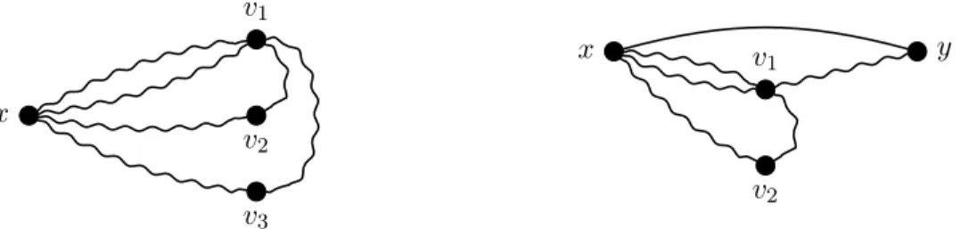
Proof. Consider two vertices x and y with four edge-disjoint paths between them. We will show that there is a pair of vertices with four internally disjoint paths between them, contradicting that G has maximal local connectivity 3. First we assume that x and y are not adjacent. Let (X, S, Y ) be a 3-separation with x ∈ X and y ∈ Y such that X is inclusion-wise minimal. Let S = {v1, v2, v3};
x v3 v2 v1 x v2 v1 y
Figure 4: The four internally disjoint xv1-paths obtained in the proof of Lemma 4.1, when x and
y are non-adjacent (left) or adjacent (right). Wiggly lines represent internally disjoint paths.
the four paths has, when going from x to y, a last vertex in X ∪ S. This vertex has to be in S, so we can assume, without loss of generality, that v1 is the last such vertex of at least two of the four
edge-disjoint paths. This means that v1 has at least two neighbours in Y .
We will show that there are four internally vertex-disjoint paths in G[X ∪ S]: two xv1-paths,
an xv2-path and an xv3-path. Let G0 be the graph obtained from G[X ∪ S] by introducing a new
vertex v01 that is adjacent to every neighbour of v1 in X ∪ S. If G0 contains four paths connecting
x and S0 := {v1, v01, v2, v3} that meet only in x, then the required four paths exist in G[X ∪ S].
If there are no four such paths in G0, then a max-flow min-cut argument (with x having infinite capacity and every other vertex having unit capacity) shows that there is a set S∗ of at most three vertices, with x 6∈ S∗, that separate x and S0. It is not possible that S∗⊂ S0: then every vertex in
the non-empty set S0\ S∗ remains reachable from x (using that every vertex of S0 has a neighbour in X). Therefore, S∗ has at least one vertex in X and hence the set of vertices reachable from x in G0 − S∗ is a proper subset of X. It follows that S∗ implies the existence of a 3-separation
contradicting the minimality of X.
Next we prove that there are internally disjoint v1v2- and v1v3-paths in G[S ∪ Y ]. Recall that v1
has two neighbours in Y . Suppose, towards a contradiction, that given any v1v2-path and v1v3-path
in G[S ∪ Y ], these paths are not internally disjoint. Then, in G[S ∪ Y ], there is a cut-vertex w that separates v1 and {v2, v3}. Since v1 has two neighbours in Y , there is a vertex q ∈ Y that is
adjacent to v1 and distinct from w. As w is a cut-vertex in G[S ∪ Y ], every qv2- or qv3-path passes
through w. Hence {w, v1} separates q from x in G, contradicting 3-connectivity.
Now there are internally disjoint xv1-, xv1-, xv2-, and xv3-paths in X and internally disjoint
v1v2- and v1v3-paths in Y . Thus, as shown Figure 4, there are four internally disjoint xv1-paths,
contradicting the fact that the local connectivity κ(x, v1) is at most 3.
A similar argument applies when x and y are adjacent. In this case, G\xy has a 2-vertex cut. Let (X, S, Y ) be a 2-separation of G\xy with x ∈ X and y ∈ Y such that X is inclusion-wise minimal, and let S = {v1, v2}. Since G\xy is 2-connected, v1 and v2 each have a neighbour in
X and a neighbour in Y . Each of the three xy-paths in G\xy has a last vertex in S, so we may assume, without loss of generality, that v1 is the last vertex of at least two of the three, and hence
v1 has at least two neighbours in Y . Let G0 be the graph obtained from G[X ∪ S] by introducing
a new vertex v01 that is adjacent to every neighbour of v1 in X ∪ S, and let S0 = {v1, v01, v2}. If
G0 does not contain three paths from x to S0 that meet only in x, then, by a max-flow min-cut argument as in the case where x and y are not adjacent, we deduce there is a set S∗ of at most two vertices that separate x and S0. Since S∗6⊂ S0, this contradicts the minimality of X.
Figure 5: A 4-connected graph with maximal local connectivity 4, but maximal local edge-connectivity 5.
not. Then, in G[Y ∪ S], there is a cut-vertex w that separates v1 and {v2, y}. Since v1 has at
least two neighbours in Y , one of these neighbours q is distinct from w. As every qv2- or
qy-path in G[Y ∪ S] passes through w, it follows that {w, v1} separates q from x in G, contradicting
3-connectivity. This completes the proof of Lemma 4.1.
At this juncture, we observe that the proof of Lemma 4.1 relies on properties specific to 3-connected graphs with local connectivity 3. For k ≥ 4, a k-3-connected graph with maximal local connectivity k may not have maximal local edge-connectivity k; an example is given in Figure 5.
Theorem 1.4 now follows immediately from Theorem 1.2, Corollary 3.6, and Lemma 4.1. One might hope to generalise this result to all graphs with maximal local connectivity 3, for a result analogous to Theorem 1.3. But this hope will not be realised, unless P=NP, since deciding if a 2-connected graph with maximal local connectivity 3 is 3-colourable is NP-complete. We prove this using a reduction from the unrestricted version of 3-colourability. Given an instance of this problem, we replace each vertex of degree at least four with a gadget that ensures that the resulting graph has maximal local connectivity 3. Shortly, we describe this gadget; first, we require some definitions.
We call the graph obtained from two copies of a diamond, by identifying a pick vertex from each, a serial diamond pair and denote it D2. We call the two degree-2 vertices of D2 the ends.
A tree is cubic if all vertices have either degree one or degree three. A degree-1 vertex is a leaf ; and an edge that is incident to a leaf is a pendant edge, whereas an edge that is incident to two degree-3 vertices is an internal edge.
For l ≥ 4, let T be a cubic tree with l leaves. For each pendant edge xy, we remove xy, take a copy of a diamond D and identify, firstly, the vertex x with one pick vertex of D, and, secondly, y with the other pick vertex of D. For each internal edge xy, we remove xy, take a copy of D2
and identify, firstly, the vertex x with one end of D2, and, secondly, y with the other end of D2. A
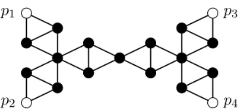
degree-2 vertex in the resulting graph T0 corresponds to a leaf of T ; we call such a vertex an outlet. We also call T0 a hub gadget with l outlets. Observe that for any integer l ≥ 4, there exists a hub gadget with exactly l outlets. When T0 is used to replace a vertex h, we say T0 is the hub gadget of h. An example of a hub gadget with four outlets is shown in Figure 6.
Proposition 4.2. The problem of deciding if a 2-connected graph with maximal local connectivity 3 is 3-colourable is NP-complete.
Proof. Let G be an instance of 3-colourability. We may assume that G is 2-connected. For each v ∈ V (G) such that d(v) ≥ 4, we replace v with a hub gadget with outlets p1, p2, . . . , pd(v),
p1
p2
p3
p4
Figure 6: A hub gadget with four outlets p1, p2, p3 and p4.
such that each neighbour ni of v in G is adjacent to pi, for i ∈ {1, 2, . . . , d(v)}. Thus each outlet
has degree three in the resulting graph G0.
It is clear that G0 is 2-connected. Now we show that G0 has maximal local connectivity 3. Clearly κ(x, y) ≤ 3 if d(x) ≤ 3 or d(y) ≤ 3. Suppose d(x), d(y) ≥ 4. Then x and y belong to a hub gadget and are not outlets. So x belongs to either two or three diamonds, each with a pick vertex distinct from x. Let P be the set of these pick vertices. When y /∈ P , an xy-path must pass through some p ∈ P , so κ(x, y) ≤ 3 as required. Otherwise, x and y are pick vertices of a diamond D, and there are two internally vertex disjoint xy-paths in D. But D is contained in a serial diamond pair D2, and all other xy-paths must pass through the end of D2 distinct from x
and y. So κ(x, y) ≤ 3, as required.
Suppose G is 3-colourable and let φ be a 3-colouring of G. We show that G0 is 3-colourable. Start by colouring each vertex v in V (G) ∩ V (G0) the colour φ(v). For each hub gadget H of G0 corresponding to a vertex h of G, colour every pick vertex of a diamond in H the colour φ(h). Clearly, each outlet is given a different colour to its neighbours in V (G) since φ is a 3-colouring of G. The remaining two vertices of each diamond contained in H have two neighbours the same colour φ(h), so can be coloured using the other two available colours. Thus G0 is 3-colourable.
Now suppose that G0is 3-colourable. Each pick vertex of a diamond must have the same colour in a 3-colouring of G0, so all outlets of a hub gadget have the same colour. Let H be the hub gadget of h, where h ∈ V (G). We colour h with the colour of all the outlets of H in the 3-colouring of G0. For each vertex v ∈ V (G) ∩ V (G0), we colour v with the same colour as in the 3-colouring of G0, thus obtaining a 3-colouring of G.
A similar approach can be used to show that 3-colourability remains NP-complete for (k−1)-connected graphs with maximal local edge-connectivity k, for any k ≥ 4. To prove this, we first require the following lemma:
Lemma 4.3. Let k ≥ 3 and j ≥ 1. Then k-colourability remains NP-complete when restricted to j-connected graphs.
Proof. We show that colourability restricted to j-connected graphs is reducible to k-colourability restricted to (j +1)-connected graphs, for any fixed j ≥ 1. Let G0 be a j-connected
graph; we construct a (j + 1)-connected graph G0 such that G0 is k-colourable if and only if G0 is.
Let S0 be a j-vertex cut in G0, let s ∈ S0, and let G1 be the graph obtained from G0by introducing
a single vertex s0 with the same neighbourhood as s. Now if S0 is a j0-vertex cut in G1, for j0 ≤ j,
then S0, or S0 \ {s0}, is a j0-vertex cut, or (j0 − 1)-vertex cut, in G0. Since S0 is not a j-vertex
cut in G1, it follows that G1 has strictly fewer j-vertex cuts than G0. Repeat this process for each
.. . .. . .. . .. . .. . Bk−1 B3 B2 B1 b1 b2 b3 .. . bk−1 u1 u2 u3 .. . uk−a (a) Gl,k, with l ≤ (k − 2)(k − 1) .. . .. . .. . .. . .. . Bk−1 B3 B2 B1 b1 b2 b3 .. . bk−1 u1 u2 (b) Hl,k, with l > (k − 2)(k − 1)
Figure 7: Gadgets and intermediate gadgets used in the proof of Proposition 4.4.
has no vertex cuts of size at most j, so G0 is (j + 1)-connected. Moreover, it is straightforward to verify that G0 is k-colourable if and only if G0 is k-colourable.
We perform a reduction from k-colourability restricted to (k − 1)-connected graphs (which is NP-complete by Lemma 4.3). Let G be a (k − 1)-connected graph. For each vertex v with d(v) ≥ k + 1, we will “replace” it with a gadget in such a way that the resulting graph G0 remains (k − 1)-connected, G0 is 3-colourable if and only if G is 3-colourable, and no vertex of G0 has degree greater than k.
We will describe, momentarily, a gadget Gl,k used to replace a vertex v of degree l, where l > k,
with vertices x1, x2, . . . , xl∈ V (Gl,k) called the outlets of Gl,k. Let Gl,k be a gadget, and let G be
a graph with a vertex v of degree l > k. We say that we attach Gl,k to G at v when we perform the
following operation: relabel the vertices of G such that V (G) ∩ V (Gl,k) = NG(v) = {x1, x2, . . . , xl},
and construct the graph (G ∪ Gl,k) − {v}.
We now give a recursive description of Gl,k. First, suppose that l ≤ (k − 2)(k − 1). Let
a = dl/(k − 1)e, and let (B1, B2, . . . , Bk−1) be a partition of {x1, x2, . . . , xl} into k − 1 cells of size
a − 1 or a. We construct Gl,k starting from a copy of the complete bipartite graph Kk−1,k−a where
the vertices of the (k − 1)-vertex partite set are labelled b1, b2, . . . , bk−1, and the remaining vertices
are labelled u1, u2, . . . , uk−a. Since k ≥ 4 and 2 ≤ a ≤ k − 2, we have k − a ≥ 2. Add an edge u1u2,
and for each i ∈ {1, 2, . . . , k − 1} and w ∈ Bi, add an edge wbi. We call the resulting graph Gl,k
and it is illustrated in Figure 7(a).
Now suppose l > (k − 2)(k − 1). Let (B1, B2, . . . , Bk−1) be a partition of {x1, x2, . . . , xl} such
that |Bi| = k − 2 for i ∈ {1, 2, . . . , k − 2}, and |Bk−1| > k − 2. Take a copy of Kk−1,1,1, labelling
the vertices of the (k − 1)-vertex partite set as b1, b2, . . . , bk−1, and the other two vertices u1 and
u2. For each i ∈ {1, 2, . . . , k − 1}, and for each w ∈ Bi, we introduce an edge wbi. Label the
resulting graph Hl,k; we call Hl,k an intermediate gadget (see Figure 7(b)). Let l1 = dHl,k(bk−1).
Since l1 = l − (k − 2)2+ 2, we have k + 1 ≤ l1 ≤ l − 2. The graph Gl,k is obtained by attaching
Gl1,k to Hl,k at bk−1. An example of such a gadget, for l = 10, k = 4, is given in Figure 8, and the
x1 x2 x3 x4 x5 x6 x7 x8 x9 x10
Figure 8: An example of a gadget, G10,4.
x1 x2 x3 x4 x5 x6 x7 x8 x9 x10 u1 u2 (a) H10,4 x5 x6 xx7 8 x9 x10 u1 u2 u01 u02 (b) H8,4 x7 x8 x9 x10 u01 u02 (c) G6,4
Proposition 4.4. For any fixed k ≥ 4, the problem of deciding if a (k − 1)-connected graph with maximal local edge-connectivity k is 3-colourable is NP-complete.
Proof. Let G be a (k − 1)-connected graph, and let G0 be the graph obtained by attaching a gadget Gd(v),k to G at v for each vertex v of degree at least k + 1. It is not difficult to verify that G0 can
be constructed in polynomial time and that every vertex of G0 has degree at most k, so G0 has maximal local edge-connectivity k. Moreover, for all distinct i, j ∈ {1, 2, . . . , k − 1}, the vertices {bi, bj, u1, u2} induce a diamond in G0, so the pick vertices {b1, b2, . . . , bk−1} of these diamonds must
have the same colour in a 3-colouring of G0. Now, given a 3-colouring of G0, we can 3-colour G, where a vertex v ∈ V (G) replaced by a gadget Gl,k in G0 is given the colour shared by the vertices
{b1, b2, . . . , bk−1} of Gl,k. It is also straightforward to verify that if G is 3-colourable, then G0 is
3-colourable.
It remains to show that G0 is (k − 1)-connected. We may assume, by induction, that G0 is obtained from G by attaching one gadget Gl,k. Moreover, when l > (k − 2)(k − 1), we
can view the attachment of a gadget Gl,k as a sequence of attachments of intermediate gadgets
Hl0,k, Hl1,k, Hl2,k, . . . , Hls−1,k, Gls,k where l = l0 and li = li−1− (k − 2)
2 + 2 for i ∈ {1, 2, . . . , s},
and ls ≤ (k − 2)(k − 1). We need only to show that the attachment of a gadget Gl,k, or of an
intermediate gadget Hl,k, preserves (k − 1)-connectivity.
Loosely speaking, we start by proving that the gadget, or intermediate gadget, itself is suffi-ciently connected. Let l > k ≥ 4. If l ≤ (k − 2)(k − 1), then set Jl,k = Gl,k, otherwise set Jl,k= Hl,k.
Let Kl be a copy of the complete graph with vertex set NG(v) = {x1, x2, . . . , xl}. We will prove
that Jl,k0 = Jl,k∪ Klis (k − 1)-connected. Let (X, Z, Y ) be a j-separation of Jl,k0 , for some j < k − 1,
such that Z is a minimal vertex cut. Set U = {u1, u2} if Jl,k = Hl,k and U = {u1, . . . uk−a} if
Jl,k = Gl,k. Suppose u1 ∈ X. Then N (u1) = {b1, b2, . . . , bk−1} ∪ {u2} is contained in X ∪ Z. If
|U | ≥ 3 and there exists u ∈ U \ {u1, u2} such that u ∈ Y , then N (u) = {b1, b2, . . . , bk−1} ⊆ Z,
contradicting |Z| < k − 1. So U ∪ {b1, . . . , bk−1} ⊆ X ∪ Z and thus Y ⊆ {x1, x2, . . . , xl}. For
i = 1, . . . , k − 1, either bi ∈ Z or Bi⊆ Z, so |Z| ≥ k − 1, a contradiction. Now we may assume that
u1 ∈ Z and, by symmetry, u2∈ Z. Since Z is minimal, u1 has a neighbour in X and a neighbour in
Y . Suppose bi∈ X and bj ∈ Y for i, j ∈ {1, 2, . . . , k − 1}. In order for Z to separate bi and bj, we
require U ∪ Bi⊆ Z or U ∪ Bj ⊆ Z, so |Z| ≥ k − 1, a contradiction. Thus Jl,k0 is (k − 1)-connected.
We now return to proving that G0 is (k − 1)-connected. Suppose, towards a contradiction, that G0 is not (k − 1)-connected. Let (X, Z, Y ) be a j-separation of G0 for some j < k − 1, such that Z is a minimal vertex cut. We denote by G0l,k the subgraph of Gl,k obtained by deleting the vertices
in common with G, namely NG(v). Note that V (G0) is the disjoint union of V (G − v) and V (G0l,k).
First, suppose that Z ⊆ V (G − v). Since G0l,k is connected, and Z ⊆ V (G − v), we deduce that, without loss of generality, V (G0l,k) ⊆ Y . It follows that Z is a j-vertex cut that separates X from (Y \ V (G0l,k)) ∪ {v} in G; a contradiction.
Now suppose that Z * V (G−v). Moreover, suppose that X ∩V (G−v) and Y ∩V (G−v) are both non-empty. Then Z ∪V (G0l,k) separates X ∩V (G−v) from Y ∩V (G−v) in G0, so (Z \V (G0l,k))∪{v} is a vertex cut of G and since Z * V (G), we have |(Z \ V (G0l,k)) ∪ {v}| ≤ j < k − 1, a contradiction
to the fact that G is (k − 1)-connected. Thus, either X ⊆ V (G0l,k) or Y ⊆ V (G0l,k). Assume without loss of generality that X ⊆ V (G0l,k) and V (G − v) ⊆ Y ∪ Z. Since |NG(v)| ≥ k, Y ∩ NG(v) 6= ∅.
Hence Z ∩ (V (G0l,k) ∪ NG(v)) separates Y ∩ (V (G0l,k) ∪ NG(v)) from X in Jl,k0 , a contradiction.
Proposition 1.5 now follows from Proposition 4.2 and Proposition 4.4. Note that Proposition 4.4 rules out (unless P=NP) the possibility of a polynomial-time algorithm that computes the
chro-matic number (or finds an optimal colouring) for a graph with maximal local edge-connectivity k, for k ≥ 4. However, there may exist a polynomial-time algorithm that, given such a graph, finds a k-colouring or determines that none exists. Thus, a result in the style of Theorem 1.3 that charac-terises when graphs with maximal local edge-connectivity 4 are 4-colourable remains a possibility.
5
Minimally k-connected graphs
In this section we prove that deciding if a minimally k-connected graph is k-colourable is NP-complete. To do this, we perform a reduction from the following problem, where k is a fixed integer at least three. A hypergraph is k-uniform if each hyperedge is of size k.
k-uniform hypergraph k-colourability Instance: A k-uniform hypergraph H.
Question: Is there a k-colouring of H for which no edge is monochromatic?
The problem of deciding if a hypergraph is 2-colourable is well known to be NP-complete [17], and the search problem of finding a k-colouring for a k-uniform hypergraph, for k ≥ 3, is shown in [7] to be NP-hard, even when restricted to such hypergraphs that are (k−1)-colourable. However, to the best of our knowledge, no proof that k-uniform hypergraph k-colourability is NP-complete has been published, so we provide one here for NP-completeness.
Proposition 5.1. The problem k-uniform hypergraph k-colourability is NP-complete for fixed k ≥ 3.
Proof. Let V1, V2, . . . , Vk be k disjoint sets each consisting of k distinct vertices, and let H0 be the
k-uniform hypergraph with vertex set V1∪ V2∪ · · · ∪ Vk whose hyperedges consist of all k-element
subsets of V (H0) not in {V1, V2, . . . , Vk}. Then, in a k-colouring of H0, for each subset X of V (H0)
of size at least k, either X is not monochromatic or X is one of V1, V2, . . . , Vk. It follows that a
k-colouring of H0 is unique, up to a permutation of the colours: each Vi, for i ∈ {1, 2, . . . , k}, is
monochromatic, and for distinct i, j ∈ {1, 2, . . . , n}, the colours given to vi ∈ Vi and vj ∈ Vj are
distinct.
We perform a reduction from k-colourability. Let G be a graph. We construct a k-uniform hypergraph H as follows. Start with the hypergraph on the vertex set V (H0) ∪ V (G), where V (H0)
and V (G) are disjoint, and containing all the hyperedges of H0. For each edge uv of G and each
i ∈ {1, 2, . . . , k}, introduce a hyperedge consisting of u, v, and k − 2 vertices of Vi. Each such
hyperedge enforces that in a k-colouring of H, the vertices u and v do not both have colour i. Thus, if H is k-colourable, then G is k-colourable. Now suppose that φ is a k-colouring of G. Then, by assigning a vertex v ∈ V (G) the colour φ(v) in H, and colouring each vertex v ∈ V (H0) the
colour i if v ∈ Vi, we obtain a k-colouring of H. This completes the proof.
Proof of Proposition 1.6. We perform a reduction from k-uniform hypergraph k-colourability. Let H be a k-uniform hypergraph with vertex set {v1, v2, . . . , vh}. We
will construct a minimally k-connected graph G with {v1, v2, . . . , vh} ⊆ V (G). For each hyperedge
e = u1u2· · · uk, where ui ∈ {v1, v2, . . . , vh} for i ∈ {1, 2, . . . , k}, let Pe be the graph on 2k vertices
that is the union of the complete graph Kk on the vertices {k1, k2, . . . , kk}, and k vertex-disjoint
u1 u2 u3 Pe vl+1 vl+2 vl+3 Ql
Figure 10: Gadgets used in the proof of Proposition 1.6.
let Ql be the graph on 3k − 1 vertices obtained from the complete bipartite graph Kk,k−1 with
k-element partite set {b1, b2, . . . , bk} by adding k vertex-disjoint edges bivj where j ≡ i + l (mod h)
for each i ∈ {1, 2, . . . , k}. For k = 3, this graph is given in Figure 10. Finally, we obtain G from the union of the i graphs Qi, for each i ∈ {1, 2, . . . , h}, and the |E(H)| graphs Pe, for each e ∈ E(H).
Note that a vertex vi, for i ∈ {1, 2, . . . , h}, is common to Qi−k, Qi−k+1, . . . , Qi−1 (with indices
interpreted modulo h) and Pe for any hyperedge e containing vi.
Suppose we have a k-colouring for G. Then, since each vertex of a Kk subgraph is coloured a
different colour, each set of vertices {u1, u2, . . . , uk} corresponding to a hyperedge e is not
monochro-matic. So the vertex colouring of the graph G gives us a colouring of the hypergraph H where no hyperedge is monochromatic.
Now suppose we have a colouring φ of H where no hyperedge is monochromatic. Starting from the colouring on {v1, v2, . . . , vh} given by φ, we can extend this to a colouring of G as follows.
Consider a Ql subgraph. For each v ∈ {vl+1, vl+2, . . . , vl+k}, if φ(v) 6= 1, we assign the vertex
adjacent to v in Ql colour 1; otherwise, it is assigned colour 2. The remaining k − 1 vertices of Ql
can then be assigned colour 3. Now consider a Pe subgraph. Let U = {u1, u2, . . . , uk}, let C be the
set of colours φ(U ), and let σ be a permutation of C with no fixed points; such a permutation exists since no hyperedge of H is monochromatic, so |C| > 1. For each c ∈ C, pick a vertex u ∈ U with φ(u) = c, and colour the vertex adjacent to u in Pethe colour σ(φ(u)). Now each of the remaining
k − |C| uncoloured vertices can be assigned one of the k − |C| unused colours arbitrarily. So G is k-colourable if and only if H is k-colourable.
For every edge xy of G, at least one of x or y has degree k, so G\xy is at most (k − 1)-connected. Moreover, it is not difficult to see there are at least k internally disjoint paths between any pair of vertices, so G is k-connected. Hence G is minimally k-connected, as required.
6
Graphs with a bounded number of vertices of degree more
than k
In this section we prove Theorem 1.9. The proof of this result relies on a generalisation of Brooks’ theorem established independently by Borodin [4] and by Erd˝os, Rubin and Taylor [8].
A list assignment for a graph G is a function L that associates to every vertex v ∈ V (G) a set L(v) of integers that are called the colours associated with v. A degree-list-assignment of a graph G is a list assignment L such that |L(v)| ≥ dG(v) for every v ∈ V (G). An L-colouring of G is a
function c from V (G) such that, for all v ∈ V (G), we have c(v) ∈ L(v), and, for all edges uv, we have c(u) 6= c(v). A graph G is L-colourable if it admits at least one L-colouring. A graph G is degree-choosable if G is L-colourable for any degree-list-assignment L. A graph is a Gallai tree if
it is connected and each of its blocks is either a complete graph or an odd cycle.
Theorem 6.1 (Borodin [4], Erd˝os, Rubin and Taylor [8]). Let G be a connected graph. Then G is degree-choosable if and only if G is not a Gallai tree. Moreover, if G is not a Gallai tree, then there is an O(m)-time algorithm that, given a degree-list-assignment L, finds an L-colouring.
We need now to study L-colourings of Gallai trees. Let G be a Gallai tree together with a list assignment L. Suppose that G has a cut-vertex and consider a leaf block B attaching at v. We say that L is B-uniform if the list L(u) is the same for all u ∈ V (B) \ {v} and satisfies |L(u)| = d(u). When L is B-uniform, we define the list assignment LB of G − V (B − {v}) as follows: for all w 6= v, LB(w) = L(w) and LB(v) = L(v) \ L(u) for some, and thus any, u ∈ V (B) \ {v}.
Lemma 6.2. If a Gallai tree G has a cut-vertex v, a leaf block B attaching at v, and a list assignment L such that L is B-uniform, then G is L-colourable if and only if G − V (B − {v}) is LB-colourable.
Proof. We deal only with the case when B is an odd cycle (the case when B is a complete graph is similar). Up to a relabelling of the colours, we may assume that every vertex of B − {v} is assigned the list {1, 2}.
Suppose that G − V (B − {v}) is LB-colourable. In the colouring of G − V (B − {v}), the colours {1, 2} are not used for v (from the definition of LB), so they can be used to colour B − {v}, showing that G is L-colourable.
Suppose conversely that G is L-colourable. We note that B − {v} is a path of odd length and, in any L-colouring, its ends must receive colours 1 and 2, because of the parity. It follows that v is not coloured with 1 or 2. Therefore, the restriction of the colouring to G − V (B − {v}) is an LB-colouring, showing that G − V (B − {v}) is LB-colourable.
When G is a graph together with a degree-list-assignment L, we say a vertex has a long list L(v) when |L(v)| > d(v).
Lemma 6.3. There is an O(m)-time algorithm whose input is a connected graph G together with a degree-list-assignment L such that at least one vertex has a long list, and whose output is an L-colouring of G.
Proof. In time O(m), a vertex v whose list is long can be identified. The algorithm then runs a search of the graph (a depth-first search, for instance) starting at v. This gives a linear ordering of the vertices starting at v: v = v1 < v2 < · · · < vn, such that, for every i ∈ {2, 3, . . . , n}, the
vertex vi has at least one neighbour vj with j < i. The greedy colouring algorithm starting at vn
then yields an L-colouring of G.
Proposition 6.4. There is an O(m)-time algorithm whose input is a Gallai tree G together with a degree-list-assignment L, and whose output is an L-colouring of G or a certificate that no such colouring exists.
Proof. The algorithm first checks whether one of the lists is long, and if so runs the algorithm from Lemma 6.3. Otherwise the classical O(m)-time algorithm of Tarjan [24] finds the block decomposition of G.
Loop step: If G is not a clique or an odd cycle, then it has a cut-vertex v and a leaf block B attaching at v. The algorithm checks whether L is B-uniform (which is easy in time O(|V (B)|)),
and if so, as in the proof of Lemma 6.2, colours the vertices of B − {v}, removes them, updates the list L(v), and repeats the loop step again.
If B is not uniform, then the algorithm identifies in B − {v} two adjacent vertices u, u0 with different lists. So, up to swapping u and u0, there is a colour c in L(u) that is not present in L(u0). Then the algorithm gives colour c to u, removes u from G, and removes colour c from the lists of all neighbours of u. The resulting graph is a connected graph together with a degree-list-assignment, and the list of u0 is long. Therefore, we may complete the colouring by Lemma 6.3.
Hence, we may assume that the algorithm repeats the loop step until the removal of leaf blocks finally leads to a clique or an odd cycle. Then, if all lists of vertices are equal, obviously no colouring exists, and the sequence of calls to Lemma 6.2 certifies that G has no L-colouring. Otherwise, a colouring can be found by Lemma 6.3.
Proof of Theorem 1.9. Let X be the set of p vertices of degree more than k in G. We guess what could be the colouring on those vertices. There are at most kp possibilities.
For each, we check whether it can be extended to a k-colouring of the whole graph. To do so we consider H = G − X, and for every vertex v ∈ V (G) \ X, we use the list assignment L(v) given by the list of colours in {1, 2, . . . , k} that are not used on a neighbour of v in X. Clearly, |L(v)| ≥ k − |N (v) ∩ X| ≥ dH(x), so we have a degree-list-assignment.
Next we find the connected components of H in O(n + m). Then for each component C, we check if C is a Gallai tree or not. If not, then we use the O(m) algorithm of Theorem 6.1 to L-colour C. If it is a Gallai tree, then we rely on Proposition 6.4.
The running time of the algorithm described above is kpO(n + m). If k > p, then we may assume, without loss of generality, that only the first p colours are used on the p vertices of degree more than k. Therefore, we have to try only pp possibilities for colouring these vertices. Thus, we obtain an algorithm that runs in time min{kp, pp} · O(n + m).
Theorem 1.9 immediately implies a fixed-parameter tractability result.
Corollary 6.5. The problem k-colourability, when parameterized by the number of vertices of degree more than k, is FPT.
Let us consider now the problem restricted to the case when G is planar. Then only the k = 3 case makes sense: for k ≤ 2, the problem is polynomial-time solvable, while for k ≥ 4 the colouring always exists by the Four Colour Theorem. For k = 3, Theorem 1.9 gives an algorithm with running time 3p· O(n + m). On general graphs, this is essentially best possible, in the following sense. The Exponential-Time Hypothesis (ETH), formulated by Impagliazzo, Paturi, and Zane [10], implies that n-variable 3-SAT cannot be solved in time 2o(n). It is known that ETH further implies that
3-colourability on an n-vertex graph cannot be solved in time 2o(n) [15]. It follows that in the algorithm given by Theorem 1.9 for 3-colourability, the exponential dependence on p cannot be improved to 2o(p): as p is at most the number of vertices, such an algorithm could be used to
solve 3-colourability in time 2o(n) on any graph.
Corollary 6.6. Assuming ETH, there is no 2o(p) · nO(1) time algorithm for 3-colourability,
where p is the number of vertices with degree more than 3.
However, on planar graphs we can do substantially better. There are several examples in the parameterized-algorithms literature [5, 6, 12, 13, 16, 22] where significantly better algorithms are known when the problem is restricted to planar graphs, and, in particular, a square root appears in
the running time. In most cases, the square root comes from the use of the Excluded Grid Theorem for planar graphs, stating that if a planar graph has treewidth w, then it contains an Ω(w) × Ω(w) grid minor. Often this result is invoked not on the input graph itself, but on some other graph derived from it in a nontrivial way. This is also the case with this problem.
Theorem 6.7. Let G be a planar graph with at most p vertices of degree more than 3. There is a 2O(√p)(n + m)-time algorithm for 3-colouring G, or determining no such colouring exists.
Proof. Let X be the set of p vertices of degree more than 3 in G. If a component C of G − X is not a Gallai tree, then, by Theorem 6.1, we can extend a colouring of G \ C to a colouring of G in linear time (similar to the proof of Theorem 1.9). Thus, we may assume that each component of G − X is a Gallai tree. It is well known that the treewidth of a graph is the maximum treewidth of one of its blocks (see, for example, [19]). Since a planar Gallai tree has no cliques of size more than 4, and an odd cycle has treewidth 2, a planar Gallai tree has treewidth at most 3. Therefore, the deletion of X from G reduces the treewidth of the resulting graph to a constant. Let w be the treewidth of G. Since G is planar, it contains a Ω(w) × Ω(w) grid minor, so Ω(w2) vertices need to be deleted in order to reduce the treewidth of G to a constant. This implies that p = |X| = Ω(w2), or in other words, G has treewidth O(√p). Therefore, after computing a constant-factor approximation of the tree decomposition (using, for example, the algorithm of Bodlaender et al. [1] or Kammer and Tholey [11]), we can use a standard 3-colouring on the tree decomposition to solve the problem in time 2O(√p)· n.
It is known that, assuming ETH, 3-colourability cannot be solved in time 2o(
√
n) on planar
graphs [15]. This implies that the 2O(√p) factor in Theorem 6.7 is best possible: assuming ETH, it cannot be replaced by 2o(√p).
References
[1] H. L. Bodlaender, P. G. Drange, M. S. Dregi, F. V. Fomin, D. Lokshtanov, and M. Pilipczuk. An o(ckn) 5-approximation algorithm for treewidth. In Proceedings of the 54th Annual IEEE Symposium on Foundations of Computer Science (FOCS 2013), pages 499–508. IEEE Com-puter Society, 2013.
[2] B. Bollob´as. Extremal Graph Theory. Courier Dover Publications, 2004.
[3] J. A. Bondy and U. S. R. Murty. Graph theory, volume 244 of Graduate Texts in Mathematics. Springer, New York, 2008.
[4] O. V. Borodin. Criterion of chromaticity of a degree prescription. In IV All-Union Conf. on Theoretical Cybernetics (Novosibirsk), pages 127–128, 1977.
[5] R. H. Chitnis, M. Hajiaghayi, and D. Marx. Tight bounds for planar strongly connected Steiner subgraph with fixed number of terminals (and extensions). In C. Chekuri, editor, Proceedings of the Twenty-Fifth Annual ACM-SIAM Symposium on Discrete Algorithms, pages 1782–1801. SIAM, 2014.
[6] E. D. Demaine and M. Hajiaghayi. The bidimensionality theory and its algorithmic applica-tions. Comput. J., 51(3):292–302, 2008.