HAL Id: hal-01088883
https://hal.archives-ouvertes.fr/hal-01088883
Submitted on 29 Nov 2014
HAL is a multi-disciplinary open access
archive for the deposit and dissemination of
sci-entific research documents, whether they are
pub-lished or not. The documents may come from
teaching and research institutions in France or
abroad, or from public or private research centers.
L’archive ouverte pluridisciplinaire HAL, est
destinée au dépôt et à la diffusion de documents
scientifiques de niveau recherche, publiés ou non,
émanant des établissements d’enseignement et de
recherche français ou étrangers, des laboratoires
publics ou privés.
european winter windstorms causing important damages
M.-S. Deroche, M. Choux, F. Codron, P. Yiou
To cite this version:
M.-S. Deroche, M. Choux, F. Codron, P. Yiou. Three variables are better than one: Detection of
european winter windstorms causing important damages. Natural Hazards and Earth System Sciences,
European Geosciences Union, 2014, 14 (4), pp.981-993. �10.5194/nhess-14-981-2014�. �hal-01088883�
www.nat-hazards-earth-syst-sci.net/14/981/2014/ doi:10.5194/nhess-14-981-2014
© Author(s) 2014. CC Attribution 3.0 License.
Natural Hazards
and Earth System
Sciences
Three variables are better than one: detection of european winter
windstorms causing important damages
M.-S. Deroche1,2,3, M. Choux3, F. Codron2, and P. Yiou1
1Laboratoire des Sciences du Climat et de l’Environnement, UMR CEA-CNRS-UVSQ, CE Saclay l’Orme des Merisiers,
91191 Gif-sur-Yvette, France
2Laboratoire de Météorologie Dynamique, UMR CNRS-UPMC-ENS-X, Place Jussieu, Paris, France
3AXA Group Risk Management Department, Paris, France
Correspondence to: M.-S. Deroche (madeleine-sophie.deroche@lmd.jussieu.fr)
Received: 20 June 2013 – Published in Nat. Hazards Earth Syst. Sci. Discuss.: 23 August 2013 Revised: 8 February 2014 – Accepted: 5 March 2014 – Published: 24 April 2014
Abstract. In this paper, we present a new approach for de-tecting potentially damaging European winter windstorms from a multi-variable perspective. European winter wind-storms being usually associated with extra-tropical cyclones (ETCs), there is a coupling between the intensity of the sur-face wind speeds and other meso-scale and large-scale fea-tures characteristic of ETCs. Here we focus on the rela-tive vorticity at 850 hPa and the sea level pressure anomaly, which are also used in ETC detection studies, along with the ratio of the 10 m wind speed to its 98th percentile. When analysing 10 events known by the insurance industry to have caused extreme damages, we find that they share an intense signature in each of the 3 fields. This shows that the relative vorticity and the mean sea level pressure have a predictive value of the intensity of the generated windstorms. The 10 major events are not the most intense in any of the 3 variables considered separately, but we show that the combination of the 3 variables is an efficient way of extracting these events from a reanalysis data set.
1 Introduction
Extra-tropical cyclones (ETCs) are an important component of the mid-latitude atmospheric circulation. Some of the North Atlantic ETCs reach Europe, where they are respon-sible for strong wind and rainfall episodes. During the winter season, some of them can be particularly intense and gener-ate damaging windstorms over Europe. Munich Reinsurance Company (Munich Re) recently released a ranking of the 10
costliest European winter windstorms over the last 30 years (Table 1). Each of them generated more than USD 2000 mil-lion (United States Dollar) of economic losses. European in-surers are highly exposed to these extreme events, leading them to buy significant reinsurance covers in order to mit-igate their risks. Therefore, and especially in a context of climate change, there is a need to characterise ETCs asso-ciated with windstorms leading to important damages, and to measure the potential evolution in the next decades of their surface signature in terms of intensity and frequency.
The study of ETCs in current and future climate has been along two main lines. The first one is the analysis of statistics of ETCs such as areas of genesis and lysis, cyclone density and cyclone intensity. In this kind of analysis, all ETCs are detected and tracked thanks to automated algorithms. Ulbrich et al. (2009) provide a review of the existing cyclone defini-tions, leading to different detection and tracking schemes; an intercomparison of their performance can be found in Neu et al. (2013). These automated algorithms are based on the two-dimensional field of the following variables: the mean sea level pressure (MSLP), the relative vorticity at 850 hPa (RV850) or the Laplacian of the MSLP. The detection is per-formed by looking for either simple maxima of RV850 or minima of MSLP, or more complex features such as opened or closed isobars (Murray and Simmonds, 1991; Sinclair, 1997; Gulev et al., 2001; Hanley and Caballero, 2012). ETC tracking is then achieved by linking features at successive time steps, thanks to a probabilistic prediction of feature movement. All the choices and assumptions made to develop a scheme offer an analysis of the ETC characteristics from
Table 1. List of the European winter windstorms that caused more than USD 1000 million over the last 30 years. In bold are the 10 reference storms used in our study (Source: compiled by Earth Pol-icy Institute from Munich Re, “Natural Disasters: Billion-$ Insur-ance Losses”, in Louis Perroy, “Impacts of Climate Change on Financial Institutions’ Medium to Long Term Assets and Liabili-ties”, presented to the Staple Inn Actuarial Society, 14 June 2005; Munich Re, Topics Geo: Natural Catastrophes 2004, 2005, 2006, 2007, 2008, and 2009 (Munich: 2005, 2006, 2007, 2008, 2009, and 2010)).
Year Winter storm Insured losses Economic losses name
USD million, original values
Oct 1987 87J 3100 3700 Jan 1990 Daria 5100 6800 Feb 1990 Herta 1300 1950 Feb 1990 Vivian 2100 3200 Feb 1990 Wiebke 1300 2250 Dec 1999 Anatol 2350 2900 Dec 1999 Lothar 5900 11 500 Dec 1999 Martin 2500 4100 Oct 2002 Jeanett 1500 2300 Jan 2005 Erwin 2500 5800 Jan 2007 Kyrill 5800 10 000 Feb 2008 Emma 1500 2000 Jan 2009 Klaus 3000 5100 Feb 2010 Xynthia 3100 6100
different angles, but also introduce uncertainties (Neu et al., 2013). Once ETCs are detected, their intensity is usually de-termined by the value of the detection variable over the ETC lifetime. Extreme ETCs are defined as a particular class of cyclones (i.e. the ones with the highest intensity) but are not necessarily associated with strong winds or losses.
The second type of study aims at evaluating the sever-ity and losses associated with European winter windstorms (Leckebusch et al., 2007, 2008; Pinto et al., 2007, 2012; Della-Marta et al., 2009; Schwierz et al., 2010; Donat et al., 2011). In all these studies, the 10 m wind speed is used as the primary meteorological variable, either alone or together with the population density in order to assess losses. The studies of Leckebusch et al. (2007, 2012); Pinto et al. (2007); Donat et al. (2011) compute a loss function from the daily maximum 10 m wind speed and the population density. In addition, Pinto et al. (2012) separate the event severity, mea-sured by a “meteorological index”, from the economic expo-sure. The meteorological index is close to the storm severity index defined in Leckebusch et al. (2008) which takes into account the spatial extension and the duration of an event with surface wind speeds exceeding a threshold. Della-Marta et al. (2009) also derive several indices, based either on the mean or on percentiles of the wind speed field, and com-pute return periods of extreme wind events using the extreme
value theory. Schwierz et al. (2010) use the ratio of the 10 m wind speed over its local 98th percentile to detect events with criteria on intensity and spatial extension. The catalogue of events obtained is then used as an input of an insurance loss model.
The approach we present in this paper mixes both types of analysis: we aim to detect the ETCs with the highest wind-related damage potential using a triplet of meteorolog-ical variables. Our methodology is designed and calibrated through the analysis of the characteristics of 10 major events known for having caused important losses (Table 1). The de-tection relies on the 850 hPa relative vorticity and the mean sea level pressure (variables used in the first type of analy-sis) as well as on the 10 m wind speed, which is used in the second type of analysis. Indeed, the 10 major events were pri-marily extreme extra-tropical cyclones, with an intense sig-nature in the 3 variables, and became major economic events when crossing high-populated areas. Looking for similar in-tense meteorological signatures should thus lead to the de-tection of events with a potential for similarly high damages. Since the methodology is meant to be applied to the output of varied models, another key aspect is the adaptability of the detection and tracking criteria.
The paper is structured as follows: in Sect. 2, an overview of the data and the variables is given. In Sect. 3, we present the methodology and the choice of detection parameters. Fi-nally, in Sect. 4, we compare the results in different reanaly-sis data sets. Conclusions are drawn in Sect. 5. All acronyms used in the text are listed in Table A1 in the Appendix.
2 Data and variables 2.1 Data
2.1.1 Meteorological data sets
Three data sets are used in this paper. The detection method-ology is developed with the ERA Interim reanalysis data set (Dee et al., 2011) in Sect. 3. ERAI is a 6-hourly data
set at a 0.75◦×0.75◦ spatial resolution covering the
pe-riod from 1979 to 2011, provided by the European Centre for Medium-Range Weather Forecasts. In Sect. 4, two other data sets are used along with ERAI to complete the analy-sis and test the robustness of the methodology. First, we use the NCEP-DOE (NCEP2) reanalysis from NCEP/NCAR, a
6-hourly data set from 1979 to 2011 with a 2.5◦×2.5◦
spa-tial resolution (Kanamitsu et al., 2002). Second, we compute
a spatial average of ERA Interim on the NCEP2 2.5◦
resolu-tion (ERAI-2.5).
The geographical window used for the detection of events is restricted to western Europe, where most of the exposure to the windstorm peril is localised; this enables us to check our detected events against databases of insured damages. The grid points over the Genoa Gulf are masked in order to avoid
the detection of Mediterranean ETCs or local lows occurring in this part of the spatial window and that are not in the scope of this study (Fig. 1).
2.1.2 Catalogues of extreme windstorms
We consider the 10 most damaging events since 1987 ranked by Munich Re (Table 1). These events, called “reference storms” hereafter, are used as case studies in order to develop the methodology (Sect. 3). They cover a time period from 1987 to 2010 and are concentrated in the winter season from October to March. As a result, we choose to work with the 6-month winters (October–March) from 1987 to 2010 and not the whole period covered by ERA Interim or NCEP2.
In order to quantify the quality of the results, we compare the events detected with our method to the ones of the
eX-treme Wind Storm (XWS) database1. The XWS catalogue
gathers 50 European winter windstorms from 1981 to 2012. Among those 50 windstorms, 16 are associated with a loss (called insurance storms hereafter) and 34 storms are not as-sociated with a loss (named non-insurance storms). The se-lection of XWS events was performed with a wind-based
in-dex computed with ERA Interim at 0.25◦ resolution over a
wider geographical window than the one we consider. The 44 events with the highest index values were automatically selected, and 6 other events including one insurance storm (Emma, 2008) were manually added.
The XWS events are considered over the period 1987– 2010 shared with our study. The database contains 38 storms over the period with 14 insurance storms, including the 10 reference events from the Munich Re (MR) ranking and 4 others: Herta (1990), Wiebke (1990), Gero (2005) and Emma (2008). The remaining 24 non-insurance storms have an in-dex value as high as the insurance storms, although they did not cause as much damages. The ratio of events that actu-ally caused damages (i.e. 14 insurance storms) over the to-tal number of events over the period (i.e. 38 storms) is 0.37. The performance of our methodology in detecting events with high damage potential within a reduced number of non-insurance events is thus quantified by both the number of in-surance storms of the XWS catalogue that are detected with our method, and the ratio of this number over the total num-ber of detected events.
2.2 Variables
Because damages are ultimately caused by surface winds, studies on damage potential mostly rely on wind-based in-dices measuring either a proxy of loss or the severity of the event. However, the accurate reproduction of local wind maxima varies according to the considered reanalysis data sets or general circulation model. The surface winds depend on boundary-layer parameterisations, and the low spatial res-olution of some data sets may not capture smaller-scale
dy-1http://www.met.reading.ac.uk/~extws/
namical or topographical features that lead to extreme winds. Therefore, we choose here to define the damage potential of an event through the combined information content available from the 10 m wind speed and other variables that are not di-rectly linked to damages, but that may have a predictive value on the physical strength of events.
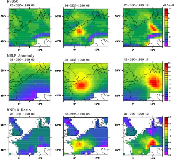
In order to characterise extra-tropical cyclones with a high potential of wind-related damages over Europe, several vari-ables at different levels of the troposphere have been anal-ysed. We favour variables that are standard outputs from models or that only require simple computation from the ini-tial data. Among all the variables considered, three are re-tained: the relative vorticity at 850 hPa, the mean sea level pressure and the 10 m wind speed. These variables are com-monly used either to detect and track ETCs (Ulbrich et al., 2009; Neu et al., 2013) or to assess potential impacts of ETCs (Leckebusch et al., 2008; Pinto et al., 2012). We briefly illus-trate in Fig. 1 the spatial patterns of these three variables in the case of the major storm Lothar (December 1999).
The relative vorticity at 850 hPa (RV850) is either directly provided in the reanalysis data set or model run, or computed as the curl of the velocity field at 850 hPa. The vorticity field is very sensitive to the spatial resolution; it becomes noisy at finer resolutions, leading to the detection of numerous and intense local-scale features (Hoskins and Hodges, 2002; Ul-brich et al., 2009; Hodges et al., 2011).
We also use the anomaly of the mean sea level pressure de-fined, at each time step, as the difference between the MSLP
and its running average over 8 days MSLP8days, see Eq. (1).
The mean sea level pressure is a large-scale field that is much less dependent on the spatial resolution than the relative vor-ticity at 850 hPa, which means that the pattern of the MSLP field remains roughly the same when upgrading the spatial resolution. Moreover, it is strongly constrained in reanalysis data sets due to the large number and quality of observation data, especially over continents. The rationale for consider-ing the anomaly of MSLP is that ETCs evolve on a more slowly varying background flow that also has large MSLP gradients. A spatial or temporal filter is often used to remove the small-scale features and the biases due to variations of the background MSLP (Hoskins and Hodges, 2002). A sim-ple temporal filter is used in our study. We first tried remov-ing the climatology of MSLP but it was not enough to brremov-ing out some of the targeted events. We thus chose to work with the running average of MSLP over 8 days, which represents the signature of the weather regime surrounding the occur-rence of ETCs (Feldstein, 2000), and has also been used by
Rivière and Joly (2006). MSLP8daysis computed at a given
time step t as the average of the MSLP over 16 time steps preceding and 16 time steps following time step t (i.e. over 32 time steps or 8 days, see Eq. 2).
Fig. 1. Maps for the three variables’ fields during the occurrence of Lothar (from 1999/12/26 00:00 UTC to 1999/12/26 12:00 UTC) in ERA Interim: first row, relative vorticity at 850 hPa (1 s−1); second row the mean sea level pressure anomaly (hPa); last row, the 10 m wind speed ratio (only grid points over land are considered). We masked the Mediterranean area of the domain.
MSLP8 days(i, j, t ) = 1 32 t +16 X t −16 MSLP(i, j, t ), (2)
where (i,j ) are the grid points coordinates and t the 4-time daily time steps.
The third variable considered is the ratio of the 10 m wind
speed to its 98th percentile (WND1098), computed for
conti-nental grid points only:
WND10ratio(i, j, t ) =
WND10 (i, j, t )
WND1098(i, j, t )
. (3)
The 10 m wind speed strongly depends on the modelling of boundary layer processes, even in the reanalyses, as well as on the time and space resolution of the outputs. Using the ratio over the 98th percentile alleviates some of these biases. This specific ratio is also often used in studies on European winter windstorms as a measure of potential damages, the
98th percentile being the threshold above which a building is at risk of being partially damaged or totally destroyed (Klawa and Ulbrich, 2003; Leckebusch et al., 2008; Schwierz et al., 2010).
Each of the three variables captures specific spatio-temporal scales and thus accounts for different aspects of extra-tropical cyclones associated with windstorms. The rel-ative vorticity at 850 hPa captures local and fast meso-scale structures, whereas the MSLP anomaly captures larger and slower-evolving systems. The ratio of the 10 m wind speed measures, at a local scale, a wind intensity that is strongly correlated with the damage potential.
3 Case study and methodology
This section presents a new method for detecting events with high wind-related damage potential in Europe. Such a method applied to a reanalysis data set should ensure the
RV850 ANOM MSLP WND10 RATIO
SET 1 SET 2 SET 3
4) LOOKING FOR COMMON EVENTS
FINAL SET
1) DETECTION
(maxima threshold: 95th perc.)
2) TRACKING
(eastward shift & distance < 900 km) 3) SELECTION
(maximum event threshold: 98th perc.)
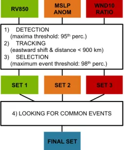
Fig. 2. Illustration of the procedure. The relative vorticity at 850 hPa (RV850), the mean sea level pressure anomaly (MSLPanom) and the 10 m wind speed ratio (WND10ratio) are used separately to detect, track and select events. The final step consists in comparing the three sets and looking for common events. An event is defined as common to the three sets if it is detected simultaneously in the three sets during at least one time step. The final set contains events that we define as events with high damage potential.
detection of events that actually generated damages and a reduced number of events that did not, for the reason that they fulfilled the intensity criteria but did not cross densely exposed areas.
The method itself and the choice of parameters are based on the case study of 10 reference storms, using the ERA In-terim data set. We describe hereafter the process, from the development of the detection methodology for a single vari-able, to the combination of the resulting per-variable events (Fig. 2). The events obtained at different stages of the process are compared to the ones of the XWS database.
3.1 Working with each variable separately
We first consider the three variables separately in our case study of the reference storms. The case study aims at answer-ing the followanswer-ing questions: do major events with important economic losses share some meteorological characteristics? How extreme is their signature within each variable? Are their economic damages reflected in the values of any of the three variables? The answers to these questions lead us to the definition of criteria specific to the detection of the the 10 reference events.
3.1.1 Definition of the detection and selection thresholds A preliminary examination of maps of the 3 variables at the time of occurrence of the 10 reference storms reveals that all
10 events display, in each of the 3 considered variables, a strong signature that singles them out from their surrounding environment when they pass across western Europe (the ex-ample of Lothar is shown in Fig. 1). Usually, ETCs detection methods select all the local maxima above a specified low threshold, because they aim to detect all cyclones that are present at a given time step within a wide region (Hoskins and Hodges, 2002). Here, since the considered area is small and we target extreme events, we choose to only retain the global maximum of each variable at each 6-hour time step.
The intensity of the 10 reference storms is compared to the distribution of the global maxima in Fig. 3. In the first row, time series of the maxima of the three variables are shown to-gether with their respective 95th percentile (red dashed line) and 98th percentile (blue line). Most of the maximum values at the time of occurrence of the 10 reference storms (coloured in green) reach the highest values. The second row of Fig. 3 shows again the maximum values of each variable, but fo-cusing on the 10 reference storms. Most values are above the 95th percentile of their respective distributions. Therefore, the 95th percentile is used as a detection threshold and only maxima higher than this threshold will be detected.
Another conclusion that can be drawn from the second row of Fig. 3 is that for each reference storm and each variable at least one value of the maxima is above the 98th percentile. This percentile is used as a selection threshold once events are formed. We will restrict our events set to events having a maximum value above the 98th percentile.
3.1.2 Single-variable methodology
The first step of the method consists in detecting maxima that have values as high as or higher than those reached by the reference storms. The maximum of each variable over the spatial window is detected at every time step; maxima with values above the 95th percentile of the time series’ distri-bution are retained. With ERA Interim, over the considered period, 840 maxima of each variable exceed this threshold.
ETCs being advected by the westerly jet stream, they usu-ally follow an eastward trajectory and their travelling speed rarely exceeds 150 km per hour. Two or more consecutive maxima above the 95th percentile are thus gathered into one same event if they follow an eastward shift and if the distance between two consecutive maxima is lower than 900 km. These two conditions enable the separation of events, such as Vivian and Wiebke (1990) or Lothar and Martin (1999) that occurred closely in time. From the 840 maxima per vari-able detected with ERA Interim, this second step leads to the generation of 214 events of relative vorticity, 203 events of mean sea level pressure anomaly and 121 events of 10 m wind speed ratio.
Finally, the selection of events with at least one maximum value above the 98th percentile further reduces the number of events per single-variable catalogues: 149 events with the relative vorticity, 117 events with the pressure anomaly and
87/8889/9091/9293/9495/9697/9899/0001/0203/0405/0607/0809/10 0 1 2 3 4 5 6 x1.e04 October−March 1987−2010 RV850 (1/s) 87/8889/9091/9293/9495/9697/9899/0001/0203/0405/0607/0809/10 −15 −5 5 15 25 35 45 October−March 1987−2010 MSLP Anomaly (hPa) 87/8889/9091/9293/9495/9697/9899/0001/0203/0405/0607/0809/10 0 0.5 1 1.5 2 2.5 October−March 1987−2010 WND10 Ratio 87J
DariaVivianAnatolLotharMartinErwinKyrillKlaus Xynthia 1 2 3 4 5 6 RV850 (1/s) x1.e04 87J
DariaVivianAnatolLotharMartinErwinKyrillKlaus Xynthia 15 20 25 30 35 40 45 MSLP Anomaly (hPa) 87J
DariaVivianAnatolLotharMartinErwinKyrillKlaus Xynthia 1 1.5 2 2.5 WND10 Ratio
Fig. 3. The first row shows the time series of the detected maxima of each variable over the time period (6-hourly time steps over October– March from 1987 to 2010, i.e. 16 768 maxima) and geographical window. The horizontal lines are the 95th (dashed red line) and 98th (blue line) quantiles of the distribution of the maxima of each variable. The second row represents the values of the maxima of each variable at the time of occurrence of the 10 reference storms. Each point for a given storm corresponds to a different 6-hourly time step during its passage.
91 events with the 10 m wind speed. The 10 reference storms are included in each set of events, but the number of events obtained in total in each single-variable catalogues remains large.
3.2 The added value of a multi-variable approach It is difficult to further reduce the total number of single-variable events while keeping the reference storms. For ex-ample, raising either the detection or selection threshold is inadequate, since some reference storms would not be tected afterwards. Another way to reduce the number of de-tected events would be to retain the top-ranked events se-lected with one variable. However, the reference storms are not top-ranked in any of the three variables, and their ranking does not follow the ranking of the damages they caused (Ta-ble 2). This is also the case in the XWS database where the insurance storms are not the 50 most extreme events, with Emma ranked 63rd – below events that did not cause dam-ages. The use of a threshold on the ranking would thus be hazardous with the perspective of using other models. This result was also highlighted in Pinto et al. (2012) who showed that the ranking of storm intensity is model-dependent.
Table 2. The 10 reference storms, ranked in the second column ac-cording to the insured losses (Munich Re), and from the third to the fifth column, their ranking according to the maximum value they reach in ERA Interim in terms of relative vorticity at 850 hPa (RV850), anomaly of the mean sea level pressure (MSLPanom) and 10 m wind speed ratio (WND10ratio). For example, with the relative vorticity at 850 hPa (RV850), we detect 149 events that we ranked according to the maximum of RV850, reached during the period they are detected over the window.
Event Munich Re RV850 MSLPanom WND10ratio
Lothar 1 32 57 2 Kyrill 2 43 15 30 Daria 3 19 12 25 87J 4 2 9 11 Xynthia 5 22 49 28 Klaus 6 51 59 1 Martin 7 6 6 3 Erwin 7 39 38 8 Anatol 8 1 7 19 Vivian 9 62 2 39
157 116 101 34 61 33 21 149 117 91 37 48 41 24 143 109 150 59 44 48 32 ERAI ERAI-2.5 NCEP2
RV850 MSLP Anomaly WND10 Ratio
Fig. 4. For each reanalysis data set: total number of events detected with each variable, number of events common to pairs of variables and number of events common to the three variables. For example, with ERAI, 149 events are detected with the relative vorticity at 850 hPa (RV850), 117 with the mean sea level pressure anomaly (MSLPanom) and 91 with the 10 m wind speed ratio. Overall, 48 events are common to RV850 and MSLPanom, 41 to MSLPanom and WND10ratio, 37 to WND10ratioand RV850. Finally, 24 events are common to the 3 variables (i.e. they are detected simultaneously with the 3 variables during at least 1 time step).
Even though the 10 reference storms are not the top-ranked events of any variable, they are selected with each of them. This is not always the case for other events of the single-variable catalogues. The complementarity of the three vari-ables is further analysed in the first panel of Fig. 4, which shows the number of events common to sets generated with different variables. The definition of a common event be-tween two variables is as follows: if two events generated and selected separately with two variables share a common time step, we consider them to actually exhibit the signature of the same event in each variable respectively.
In ERAI, the number of common events between pair-wise variables is less than half the number of events selected with each variable separately. Considering events common to the 3 variables further reduces that number to 24, including the 10 reference storms (see Fig. 4, first panel). Figure 5 shows 3 of the 24 final events: 1 XWS insurance storm (87J, 1987), 1 XWS insurance storm (Quinten, 2009) and 1 non-insurance storm detected with our method (December 1998). We show for each event detected the position of the maxi-mum of the relative vorticity (grey points) and of the anomaly of mean sea level pressure (red stars), as well as the footprint of the 10 m wind speed ratio with values above 1. The foot-print is computed at each grid cell of the spatial window as the maximum of the 10 m wind speed ratio over the time pe-riod that the event is detected with this variable. Final events are not necessarily detected at each time step with each of the three variables. For example, Quinten (2009) is first detected with both the relative vorticity and the anomaly of mean sea level pressure before being detected with the three variables over two time steps, and finally with the anomaly of mean sea level pressure and 10 m wind speed over the fourth time step.
Table 3. Number of events detected with one variable (RV850, MSLPanom, WND10ratio), and events common to the three cata-logues (MULTI). Columns show the XWS insurance events, the to-tal number of events and the resulting ratio. The ERAI, ERAI-2.5 and NCEP2 data sets are used, and the XWS catalogue numbers are shown for comparison.
Data set Variable XWS insurance Total number Ratio
events of events ERAI RV850 12 149 0.08 MSLPanom 12 117 0.10 WND10ratio 14 91 0.15 MULTI 11 24 0.46 ERAI-2.5 RV850 12 157 0.08 MSLPanom 12 116 0.10 WND10ratio 14 101 0.14 MULTI 11 21 0.52 NCEP2 RV850 12 140 0.09 MSLPanom 11 121 0.09 WND10ratio 13 150 0.09 MULTI 9 33 0.27 XWS 14 38 0.37
The three events reached the same intensity but they affected different areas with different exposures to the peril, and thus caused different levels of damages.
3.3 Comparison to the XWS catalogue
Table 3 summaries the comparison between the events gen-erated for each variable, the final common events and the in-surance storms of the XWS database. The ratio of detected insurance storms over the total number of detected events is also presented.
The results show that the 14 insurance storms of the XWS database are detected with the 10 m wind speed ratio. How-ever, the ratio of insurance storms over the total number of events is then 0.15, which is much lower than the XWS ra-tio 0.37. With the relative vorticity and the anomaly of mean sea level pressure, 12 insurance storms are detected, with a ratio of 0.08 and 0.10 respectively. The missing insurance storms within the relative vorticity set of events are Gero (2005) and Emma (2008), because their trajectory is further north than the spatial window we consider. Within the set of events derived from the anomaly of mean sea level pressure, Herta (1990) and Gero (2005) are missing: Herta because the values of the anomaly of mean sea level pressure are lower than the detection thresholds, Gero because its track is fur-ther north than our spatial window spatial window. We actu-ally capture the values at the boundary of the event which are lower than our thresholds.
Among the final common events, there are 11 insurance storms of the XWS catalogue and the ratio over the total
1.0 1.2 1.4 1.6 1.8 2.0 + + + + 10m Windspeed Ratio 1987−10−15 06 to 1987−10−16 12 1.0 1.2 1.4 1.6 1.8 2.0 + + + 10m Windspeed Ratio 2009−02−10 00 to 2009−02−10 12 1.0 1.2 1.4 1.6 1.8 2.0 + ++ 10m Windspeed Ratio 1998−12−20 06 to 1998−12−21 00
Fig. 5. Three of the final events detected with the method in ERA Interim: one XWS insurance storm (87J, 1987), one XWS non-insurance storm (Quinten, 2009) and one non-insurance storm detected (December 1998). Grey dots represent the maxima detected with the relative vorticity, the red stars the maxima detected with the anomaly of mean sea level pressure, and the coloured shade is the footprint of 10 m wind speed ratio over the detection dates; only values above 1 are represented. Maxima of variables happening at the same time are linked by a black line.
number of detected events is now up to 0.46. It should be noted that the spatial window used to select the XWS events is wider than ours, which partly explains the lower value of the XWS ratio. Hence it is more likely to detect non-insurance events within a wide window than within a small one. Three insurance storms are missed: Herta (1990), Gero (2005) and Emma (2008), as anticipated with the events gen-erated with the single-variable methodology. The other 13 events of the 24 final events include 5 XWS non-insurance storms and 8 other events. Among these 8 events, one oc-curred in December 1998 and is referenced in Mayencon (2000), a second one lead to the Prestige oil spill (13 Novem-ber 2002) and a third one is the named storm Johanna (10 March 2008).
3.4 Sensitivity to the size of the spatial window
The comparison with the XWS storms showed the impact of the spatial offset that exists between a low-pressure system and its associated maximum wind speed. The spatial win-dow was chosen to minimise that effect, that is, it should extend enough northward to capture the low-pressure cen-tres associated with extreme winds over areas of western Eu-rope with high exposition, roughly Great Britain, France and Germany. However, the detection of two storms, Gero (2005) and Emma (2008), is affected by this effect since both are de-tected with the 10 m wind speed, but are missed within one of the other two variables.
We therefore test the robustness of the methodology by using a much wider window encompassing Portugal, Spain, Ireland and the Scandinavian region. It includes most of the storm track over Europe, but with less exposed areas. The strong activity occurring in the northwestern part of the larger window leads to the detection of maxima of both relative vorticity and anomaly of mean sea level pressure that reach higher values than within the smaller window. In order to
Table 4. Same as Table 3, but for a wider spatial window going from Spain to Scandinavia.
Data set Variable XWS Total number Ratio
events insurance of events ERAI RV850 13 331 0.04 MSLPanom 13 250 0.05 WND10ratio 14 220 0.06 MULTI 12 62 0.19 XWS 14 38 0.37
still detect all the reference storms, we thus lower the thresh-olds to the 90th and 95th percentiles. In addition to our pre-vious damaging events, we now detect Gero (2005) but still miss Herta (1990) and Emma (2008) because their intensity is lower than our thresholds. Widening the spatial window therefore reduces the risk of offset, at the expense of low-ering the ratio between the number of insurance storms and insurance storms (Table 4). A large fraction of the non-insurance events detected with the large window are localised over Scandinavia where, for now, there is little exposure.
The benefit of widening the spatial window, i.e. detect-ing one more insurance storm, seems small compared to the drawback of detecting many more events in total, with no possible comparison with damage databases. For the current climate and exposure, we consider the initial window ade-quate enough to capture most of the insurance storms.
To conclude on the results of Sect. 3, taking the inter-section of event sets generated with three separate variables gives more satisfying results than using a single one. Indeed, the selection of 24 events with potential for wind-related damages over the last 30 years is consistent with records from
insurance companies of major damages over the area con-sidered. The final events have been compared to the XWS database. We show that the approach is robust when con-sidering a wider window. Once the thresholds are defined from the new maxima PDFs to fit the values of the reference storms, we still detect events that generated large economic damages, along with events sharing the same intense mete-orological signature, but crossed areas with lower exposure. The robustness of the method with regard to the spatial reso-lution and data set is now tested in Sect. 4.
4 Sensitivity to data set and spatial resolution
The ultimate objective of this work is to apply the method to the outputs of general circulation models such as the ones participating in the Coupled Model Intercomparison Project (CMIP5). Most of those models have a spatial resolution coarser than ERAI, especially when run over long periods of time. In order to validate its robustness against spatial res-olution, the methodology is applied to the coarser reanalysis
data sets NCEP2 and ERAI, downgraded to the 2.5◦spatial
resolution. This will partially separate the resolution effect (ERAI versus ERAI-2.5) from the model effect (ERAI-2.5
versus NCEP2), with the caveat that downgrading to 2.5◦,
the output of a model run at 0.75◦is different from taking the
output of a model run at 2.5◦.
In this section, we aim at pointing out the added value of the approach presented in Sect. 3 when dealing with models run at different spatial resolutions. We first present the dis-tributions of the maxima of the three variables in order to analyse the differences and similarities between the reanal-ysis data sets. Then we compare single-variable and multi-variable catalogues of both ERAI-2.5 and NCEP2 to the XWS database. Finally, we analyse the catalogue of final events of each reanalysis data set in order to determine how many common events they share and conclude on the perfor-mance of the methodology.
4.1 Probability distribution functions
The probability distribution functions (PDFs) obtained from the maxima time series of each variable are plotted in Fig. 6 for ERAI, ERAI-2.5 and NCEP2. While the distributions of the MSLP anomaly and 10 m wind speed ratio are nearly identical from one data set to the other, the relative vortic-ity distributions differ. A first shift towards lower values is observed when downgrading the resolution from ERAI to ERAI-2.5 and a second one when changing the model from ERAI-2.5 to NCEP2 This stresses the added value of using intensity thresholds based on percentiles rather than absolute values in order to ensure the adaptability of the detection to different kinds of data sets.
4.2 Single-variable and multi-variable catalogues The results of the methodology are first shown in Fig. 4 with, for each reanalysis data set, the number of events generated with each of the variables, the number of common events to pair-wise variables and the number of events in the final set (i.e. events common to the three variables). The number of events common to the 3 variables is always reduced com-pared to the number of events within the catalogues of indi-vidual variables: 24 events with ERAI, 21 with ERAI-2.5 and 33 with NCEP2. Table 3 summarises the number of insur-ance storms within each single-variable and multi-variable catalogues as well as the total number of detected events and the resulting ratio. In terms of selectivity, the intersection of the three variables still leads to a higher ratio than the single-variable ratios. With ERAI-2.5, we get the same insurance storms and also miss Herta (1990), Gero (2005) and Emma (2008) for the same reasons as with ERAI. With NCEP2, the ratio is lower than the XWS ratio but remains higher than the single-variable ratios. This is explained by the fact that five insurance storms are not detected: Herta (1990), Wiebke (1990), Lothar (1999), Gero (2005) and Emma (2008).
These results highlight two issues that prevent the detec-tion of all the insurance storms with our methodology. The first one is linked to the spatial resolution: a model run at a low resolution may not be able to reproduce small-scale sys-tems such as Wiebke (1990) and Lothar (1999). The under-estimation of Lothar in NCEP2 was also mentioned in Pinto et al. (2012). Thus there is little that can be done to allow the detection of these events in such a data set. The second is-sue relates to the choice of the spatial window and the risk of missing events because of the offset between a low-pressure core and its maximum wind speed. The method was applied to a wider window and led to the detection of Gero (2005) and Emma (2008), but also a higher number of total events and a ratio of 0.15. The benefit of gaining two more insur-ance events is then lost because of the detection of a large number of final events.
4.3 Comparison of the final events between reanalysis data sets
Finally, we estimate the ability of the method to detect the same events from different data sets by computing the ratio of common events between two reanalysis data sets over the total number of events. The definition of a common event be-tween two data sets is as follows: if two final events generated and selected in two different data sets share a common time step, we consider them to actually exhibit the signature of the same event in each data set respectively. Between ERAI and ERAI-2.5, the ratio value is 0.71: 15 common events divided by 21 events of ERAI-2.5. Between ERAI-2.5 and NCEP2, there are 16 common events within the 33 events of NCEP2; the resulting ratio is thus equal to 0.48. This means that al-most half of the final events of NCEP2 are the same ones as
0 1 2 3 4 5 6 0 0.1 0.2 0.3 0.4 0.5 0.6 RV850 (1/s) Density x1.e−04 ERAI ERAI−2.5 NCEP2 −20 0 20 40 60 0 0.1 0.2 0.3 0.4 0.5 0.6 MSLP Anomaly (hPa) Density ERAI ERAI−2.5 NCEP2 0.5 1 1.5 2 0 0.1 0.2 0.3 0.4 0.5 0.6 WND10 Ratio Density ERAI ERAI−2.5 NCEP2
Fig. 6. Probability distributions of the maxima of relative vorticity at 850 hPa (RV850), mean sea level pressure anomaly (MSLP Anomaly) and 10 m wind speed ratio (WND10ratio). ERA Interim distribution curves are represented by a dark blue line, ERAI-2.5 distribution curves by a light blue line and the black dashed lines represent NCEP2 distributions.
ERAI ERAI-2.5 NCEP2
LotharKyrillDaria
87J
XynthiaKlausMartinErwinAnatolVivian
0 70 140
Rank of ev
ents
LotharKyrillDaria
87J
XynthiaKlausMartinErwinAnatolVivian
0 55 110
Rank of ev
ents
LotharKyrillDaria
87J
XynthiaKlausMartinErwinAnatolVivian
0 40 80 Rank of ev ents RV850 MSLP Anomaly WND10 Ratio
Fig. 7. Ranking of the 10 reference storms respectively using the relative vorticity at 850 hPa (RV850), the MSLP anomaly (MSLP Anomaly) and the 10 m wind speed ratio (WND10ratio). The names of the reference storms are ranked according to the MR damages.
those of ERAI-2.5. Although the two reanalysis data sets do not provide the same information in terms of extremes (e.g. small-scale systems), we succeed in detecting almost 50 % of common extreme events. To compare, Pinto et al. (2012) selected the 10 top-ranked events detected with a wind-based loss index in 2 reanalysis data sets, ERA40 and NCEP. They found that only two events were present in both cases. They highlight the difficulty of comparing extreme events, in par-ticular because because the location of high wind speeds may differ from one data set to the other.
Finally, it would not be possible to get our result by consid-ering the most intense events in one variable only. We show in Fig. 7 that the 10 reference storms are not the 10 most extreme events in any pair of reanalysis data sets and vari-ables, which generalises the result obtained with ERAI only. Additionally, the ranks of the 10 reference storms vary with the data set. For example, in order to select the 10 reference storms with the anomaly of mean sea level pressure, we must take the first 55 events with ERAI, the first 110 with ERAI-2.5 and the first 100 with NCEP2.
5 Conclusions
The methodology presented in this paper enables the detec-tion of windstorms with high damage potential. It is easily adaptable to different data sets or model outputs with differ-ent spatial resolutions. The method’s novelty lies in its ability to target European winter windstorms with a potential im-pact on insurance policies by using exclusively meteorologi-cal variables.
Its robustness comes from two main factors: the defini-tion of thresholds relative to the data set and the use of other meso- and large-scale variables in addition to the surface wind speed. The use of thresholds based on percentiles of the distribution of the variables ensures the adaptability to different data sets, especially with varying resolutions. More originally, we show that a simple approach based on several variables of different scales is as efficient as approaches using only based indices in selecting European winter wind-storms with damage potential. First, in terms of selectivity of events, we show that by taking the intersection of events se-lected with different variables separately, we not only reduce the total number of events but above all we retain most of
the damaging ones. Second, when comparing the final events obtained with two different reanalysis data sets displaying important discrepancies in the reproduction of small-scale events, half of the final events are common to the two data sets, which suggests the robustness of the method. We still miss some of the insurance storms either for intensity reasons (one or three events according to the data set) or because of the offset effect (two events). However, the modification of the criteria in order to include those events leads to a depre-ciation of the overall results.
The methodology has been developed for the ETCs asso-ciated with windstorms that could generate important dam-ages in Europe. Therefore the choice of the window and the fact that we focus on extremes allow us to make assumptions that would not be possible in other regions. However, the ap-proach we used to define the methodology can be applied to other regions and hazards. We hope this analysis will provide a new perspective on the quantification of damage potential of natural hazards.
Acknowledgements. Madeleine-Sophie Déroche is grateful to
the AXA Research Fund for the PhD grant that supports the research for this paper. The authors wish to express their gratitude to Gwendal Rivière as well as to the reviewers for their helpful comments.
Edited by: B. D. Malamud
Reviewed by: U. Ulbrich and one anonymous referee
The publication of this article is financed by CNRS-INSU.
References
Dee, D. P., Uppala, S. M., Simmons, A. J., Berrisford, P., Poli, P., Kobayashi, S., Andrae, U., Balmaseda, M. A., Balsamo, G., Bauer, P., Bechtold, P., Beljaars, A. C. M., Van de Berg, L., Bidlot, J., Bormann, N., Delsol, C., Dragani, R., Fuentes, M., Geer, A. J., Haimberger, L., Healy, S. B., Hersbach, H., Hólm, E. V., Isaksen, L., Kållberg, P., Köhler, M., Matricardi, M., McNally, A. P., Monge-Sanz, B. M., Morcrette, J.-J., Park, B.-K., Peubey, C., De Rosnay, P., Tavolato, C., Thépaut, J.-N., and Vitart, F.: The ERA-interim reanalysis: configuration and perfor-mance of the data assimilation system, Q. J. Roy. Meteor. Soc., 137, 553–597, 2011.
Della-Marta, P. M., Mathis, H., Frei, C., Liniger, M. A., Kleinn, J., and Appenzeller, C.: The return period of wind storms over eu-rope, Int. J. Climatol., 29, 437–459, 2009.
Donat, M. G., Leckebusch, G. C., Wild, S., and Ulbrich, U.: Future changes in European winter storm losses and ex-treme wind speeds inferred from GCM and RCM multi-model
simulations, Nat. Hazards Earth Syst. Sci., 11, 1351–1370, doi:10.5194/nhess-11-1351-2011, 2011.
Feldstein, S. B.: The timescale, power spectra, and climate noise properties of teleconnection patterns, J. Climate, 13, 4430–4440, 2000.
Gulev, S. K., Zolina, O., and Grigoriev, S.: Extratropical cy-clone variability in the Northern Hemisphere winter from the NCEP/NCAR reanalysis Data, Clim. Dynam., 17, 795–809, 2001.
Hanley, J. and Caballero, R.: Objective identification and tracking of multicentre cyclones in the ERA-interim reanalysis dataset, Q. J. Roy. Meteor. Soc., 138, 612–625, 2012.
Hodges, K. I., Lee, R. W., and Bengtsson, L.: A comparison of extratropical cyclones in recent reanalyses ERA-interim, NASA MERRA, NCEP CFSR, and JRA-25, J. Climate, 24, 4888–4906, 2011.
Hoskins, B. J. and Hodges, K. I.: New perspectives on the Northern Hemisphere winter storm tracks, J. Atmos. Sci., 59, 1041–1061, 2002.
Kanamitsu, M., Ebisuzaki, W., Woollen, J., Yang, S.-K., Hnilo, J. J., Fiorino, M., and Potter, G. L.: NCEP–DOE AMIP-II reanalysis (R-2), B. Am. Meteorol. Soc., 83, 1631–1643, 2002.
Klawa, M. and Ulbrich, U.: A model for the estimation of storm losses and the identification of severe winter storms in Germany, Nat. Hazards Earth Syst. Sci., 3, 725–732, doi:10.5194/nhess-3-725-2003, 2003.
Leckebusch, G. C., Ulbrich, U., Fröhlich, L., and Pinto, J. G.: Property loss potentials for European midlatitude storms in a changing climate, Geophys. Res. Lett., 34, L05703, doi:10.1029/2006GL027663, 2007.
Leckebusch, G. C., Renggli, D., and Ulbrich, U.: Development and application of an objective storm severity measure for the north-east Atlantic region, Meteorol. Z., 17, 575–587, 2008.
Mayencon, R.: La violente tempête du 20 décembre 1998, La Météorologie 8, 32, 2000.
Murray, R. and Simmonds, I.: A numerical scheme for tracking cy-clone centres from digital data. I. Development and operation of the scheme, Aust. Meteorol. Mag., 39, 155–166, 1991.
Neu, U., Akperov, M. G., Bellenbaum, N., Benestad, R., Blender, R., Caballero, R., Cocozza, A., Dacre, H. F., Feng, Y., Fraedrich, K., Grieger, J., Gulev, S., Hanley, J., Hewson, T., Inatsu, M., Keay, K., Kew, S. F., Kindem, I., Leckebusch, G. C., Liber-ato, M. L. R., Lionello, P., Mokhov, I. I., Pinto, J. G., Raible, C. C., Reale, M., Rudeva, I., Schuster, M., Simmonds, I., Sin-clair, M., Sprenger, M., Tilinina, N. D., Trigo, I. F., Ulbrich, S., Ulbrich, U., Wang, X. L., and Wernli, H.: IMILAST: A Com-munity Effort to Intercompare Extratropical Cyclone Detection and Tracking Algorithms, B. Am. Meteorol. Soc., 94, 529–547, doi:10.1175/BAMS-D-11-00154.1, 2013.
Pinto, J. G., Fröhlich, E. L., Leckebusch, G. C., and Ulbrich, U.: Changing European storm loss potentials under modified cli-mate conditions according to ensemble simulations of the ECHAM5/MPI-OM1 GCM, Nat. Hazards Earth Syst. Sci., 7, 165–175, doi:10.5194/nhess-7-165-2007, 2007.
Pinto, J., Karremann, M., Born, K., Della-Marta, P., and Klawa, M.: Loss potentials associated with European windstorms under fu-ture climate conditions, Clim. Res., 54, 1–20, 2012.
Rivière, G. and Joly, A.: Role of the low-frequency deformation field on the explosive growth of extratropical cyclones at the jet
exit, Part I: Barotropic critical region, J. Atmos. Sci., 63, 1965– 1981, 2006.
Sinclair, M. R.: Objective identification of cyclones and their cir-culation intensity, and climatology, Weather Forecast., 12, 595– 612, 1997.
Ulbrich, U., Leckebusch, G. C., and Pinto, J. G.: Extra-tropical cy-clones in the present and future climate: a review, Theor. Appl. Climatol., 96, 117–131, 2009.
Appendix A
Table A1. Table of variables and acronyms.
Variables
MSLP: Mean Sea Level Pressure
MSLP8 days: Running Average over eight days of the mean sea level pressure
MSLPanom: Mean sea level pressure anomaly RV850: Relative Vorticity at 850 hectoPascal WND10: 10 m wind speed
WND1098: 98th percentile of the 10 m wind speed, computed for each grid point over the whole given period WND10ratio: Ratio of the 10 m wind speed over its 98th percentile WND1098
Data sets
ERAI: ERA Interim
ERAI-2.5: ERA Interim downgraded at 2.5◦ NCEP2: NCEP-DOE Reanalysis 2
Other
CMIP5: Coupled Model Intercomparison Project Phase 5 ECMWF: European Centre for Medium-Range Weather Forecasts ETC: Extra-Tropical Cyclone
NCEP/NCAR: National Centre for Environmental Prediction/National Centre for Atmospheric Research PDF: Probability Distribution Function