HAL Id: hal-01935591
https://hal.archives-ouvertes.fr/hal-01935591
Submitted on 26 Nov 2018
HAL is a multi-disciplinary open access
archive for the deposit and dissemination of
sci-entific research documents, whether they are
pub-lished or not. The documents may come from
teaching and research institutions in France or
abroad, or from public or private research centers.
L’archive ouverte pluridisciplinaire HAL, est
destinée au dépôt et à la diffusion de documents
scientifiques de niveau recherche, publiés ou non,
émanant des établissements d’enseignement et de
recherche français ou étrangers, des laboratoires
publics ou privés.
François Bobot, Stéphane Graham-Lengrand, Bruno Marre, Guillaume Bury
To cite this version:
François Bobot, Stéphane Graham-Lengrand, Bruno Marre, Guillaume Bury. Centralizing equality
reasoning in MCSAT. 16th International Workshop on Satisfiability Modulo Theories (SMT 2018),
Jul 2018, Oxford, United Kingdom. �hal-01935591�
Fran¸cois Bobot
1, St´
ephane Graham-Lengrand
2, Bruno Marre
1, and Guillaume
Bury
3 1CEA LIST, Software Security Lab, Gif-sur-Yvette, France
2
CNRS, ´Ecole Polytechnique, Palaiseau, France
3
ENS Paris-Saclay, Cachan, France
Abstract
MCSAT is an approach to SMT-solving that uses assignments of values to first-order variables in order to try and build a model of the input formula. When different theories are combined, as formalized in the CDSAT system, equalities between variables and terms play an important role, each theory module being required to understand equalities and which values are equal to which. This paper broaches the topic of how to reason about equalities in a centralized way, so that the theory reasoners can avoid replicating equality reasoning steps, and even benefit from a centralized implementation of equivalence classes of terms, which is based on a equality graph (Egraph). This paper sketches the design of a prototype based on this architecture.
1
Introduction
Model-constructing satisfiability (MCSAT) [6, 11] is an approach to SMT-solving that applies the principles of Conflict-Driven Clause Learning (CDCL) not only to propositional reasoning but also to theory reasoning. For instance, the main procedure is a loop that alternates model building phases with conflict analysis phases.
MCSAT is specifically tuned to theories that have a standard model, in the sense that a (quantifier-free) formula is satisfiable in the theory if and only if it evaluates to true in this particular model for some interpretation of its free variables. The MCSAT transition system, when given an input formula to satisfy, organises the search for such an interpretation similarly to CDCL. It gradually builds a candidate interpretation by aggregating on a trail explicit assignments of truth values to Boolean variables, e.g., (l←true), but in contrast to CDCL it also aggregates explicit assignments of model values to first-order variables, e.g., (x←3/4). It
relies on a theory plugin to provide an evaluation function and to generate theory lemmas whenever the candidate interpretation fails to satisfy the input formula, a situation known as a conflict. MCSAT thus combines with Boolean reasoning any theory for which an MCSAT theory plugin can be defined, including for instance linear and non-linear versions of arithmetic [6, 8,
11], and the theory of bitvectors [5,13]. In [7], Equality with Uninterpreted Functions (EUF) is added to the combination of Linear Real Arithmetic (LRA) and Boolean reasoning, hinting at a rather systematic approach to theory combination. The full development of this approach, proving soundness, completeness and termination properties for the combination of theories with disjoint signatures, was conducted in a more general framework called CDSAT for Conflict-Driven Satisfiability [2,3]. CDSAT generically combines a collection of abstract theory modules where theory reasoning is specified in terms of inference rules rather than evaluation and theory lemmas, and therefore CDSAT does not require theories to have a standard model in the sense described above. Indeed the interpretation of sorts as sets, and of symbols as functions and
predicates, may vary according to theory models, while being more specified than in theory EUF (imagine for instance a theoryTinj whose unique function symbol f from sort s1 to sort
s2 is injective). MCSAT is an instance of CDSAT, and the more traditional Nelson-Oppen
scheme [12] for theory combination is another, where each theoryT comes with a black box procedure that decidesT -satisfiability. CDSAT can also combine MCSAT theory plugins with black box decision procedures. In all cases, the critical information exchanged between theory modules, whether explicitly or by assigning first-order values, is about equalities, i.e., which variables or terms are equal to which.
Indeed, theory combination in MCSAT raises for instance the question: if a theory module for, e.g., LRA communicates assignment x←3/4, what should another theory module in the
combination understand from it? From value 3/4 itself it should only understand that it is
different from other values, say2/3. Thus, if the LRA module communicates another assignment
y←2/3(resp. y←3/4), other theory modules only have to understand that x and y are different
(resp. equal). Each theory module is therefore required to understand equality and reason about it taking into account reflexivity, symmetry and transitivity. In practice though, it is desirable to avoid duplicating computation for equality reasoning across different theory modules.
In this paper, we sketch the design of an architecture based on MCSAT where equality reasoning is centralized. A unique component implementing an equality graph (Egraph) lies at the centre of the architecture, and can be queried by the different theory modules.
On the one hand, this departs from the traditional SMT-solving architecture based on DPLL(T), where the SAT-solver, rather than the Egraph, has the central role. Instead, we follow the idea of MCSAT and CDSAT that Boolean reasoning can be considered as one of the theories to be combined, and we argue that it is more important for theory modules to be directly interfaced with the Egraph, delegating equality reasoning to it, rather than to be interfaced with the module handling Boolean connectives.
On the other hand, the literature on MCSAT and CDSAT hardly investigates whether and how the mechanisms controlling the assignments of values to terms can be usefully enhanced by centralizing equality reasoning: For instance, assume that terms t0, . . . , tn are equal, i.e.,
assume the connectivity of the graph whose vertices are those terms and whose edges are the explicitly known equalities ti= tj between them. There is a risk in MCSAT and CDSAT that
deciding the assignment of a value to t0 triggers n further assignments of the same value to
t1, . . . , tn, via the equality constraints between the terms which, one after the other, all become
unit constraints. On the contrary, not performing those n propagations may be problematic, say if the value of t42 is needed for the evaluation of a bigger term where t42 occurs.
In this paper we sketch how to leverage an Egraph in order to avoid such dilemmas and provide other benefits such as recording the domains of feasible values for equivalence classes of terms rather than for individual terms. The use of the Egraph during the model building phases, described in Section2, then impacts how conflict analysis is also performed, as described in Section3. A prototype is available athttps://github.com/witan-org/witan.
2
Model building
As in CDCL, MCSAT, and CDSAT, the model building phase consists in making decisions about the model to be built, and propagating the consequences of these decisions to further complete the construction of the model. This section describes how the equality reasoner is used during that phase.
2.1
Purpose and general principles of the equality reasoner
The equality reasoner has several purposes:
The first one is to make available, on demand, the information of whether two terms are equal, different, or whether this is unknown, given the knowledge that has been passed to the reasoner so far. This takes into account reflexivity, symmetry, and transitivity, but also (this is specific to MCSAT/CDSAT) the assignment of values to variables and more generally to terms: If x←3/4, y←3/4, z←2/3have been communicated to the equality reasoner, then the reasoner can
tell (without understanding the semantics of3/4and2/3) that x is equal to y and different from
z. This inference power is formally identified in [2, 3], in the form of equality inferences. The second purpose is to make available, on demand, the information of whether a term has a determined value (and if so, which one), either because a value has been assigned to it explicitly, or because a value has been explicitly assigned to another term that is equal to the first one according to equality inferences.
The third one is to record theory-specific information about terms that is meant to be invariant across classes of terms that are known to be equal. For instance, imagine the LRA theory module records that the range of feasible values for a variable x is in the interval[2/3,3/4]
(e.g., any other value would violate a constraint that must be satisfied), and wonders about the range of feasible values for variable y. If y can be inferred to be equal to x according to equality inferences, then the feasible values for y should also be in[2/3,3/4]. This is particularly
useful in MCSAT, where theory plugins often maintain, for each variable whose value is to be determined, a domain of feasible values to pick from. Maintaining one domain for each equivalence class of terms, rather than for each term or variable, is likely to be more efficient, and can be provided by the equality reasoner.
For obvious reasons of efficiency, an equality reasoner that makes all of this information available should avoid eager computations. For reflexivity, symmetry and transitivity, an Egraph based on union-find is the obvious and well-known structure to use, materialising equivalence classes of terms. Making the equality reasoner handle value assignments, so as to capture all equality inferences, only requires a minor adaptation: both terms and values can form nodes of the Egraph, and when x←3/4 is communicated to the reasoner, the equivalence classes of x
and3/4should be merged. The Egraph can record, for each equivalence class, the value (if any)
that has been assigned to some term in the class, and otherwise the domain of feasible values. This allows the Egraph to fulfil the second and third purpose, and detect when merges lead to basic inconsistencies: for instance if in the example above some term in the same class as x has already been assigned a different value, say2/3, the merge fails and a conflict is raised.
Finally, making all of this information available on demand means that the Egraph can be queried for a direct answer, but also that whichever component sends the query can also ask to be notified when the answer to the query changes in the future: typically, if two terms cannot be determined to be equal or different according to equality inferences, being notified when their equality becomes determined may be useful for a theory module. The Egraph therefore allows components to subscribe to a daemon monitoring the query.
In the next section we further detail the implementation and use of the Egraph, describing the objects that are manipulated, how theories could propagate information or be warned that some information have been propagated, and finally how the engine orders these request.
2.2
Implementation and use of the Egraph
Nodes A node of the Egraph is an inhabitant of an OCaml sum type, being either a term, of type ThTerms, or a value, of type Values. Both are hashconsed in our implementation.1 Since each theory module can use its own notion of value, the inhabitants of Values can be heterogeneous, implementing the Booleans (⊺, ), the rationals (for LRA), the algebraic reals (for NRA), etc. Type Values is actually an extensible type, so that it can be defined at runtime according to which theory modules participate to the theory combination. The requirement to hashcons the Values just means that an equality function (already needed) and a hash function (for limiting the use of the equality) must be provided, so even with complicated values such as the algebraic reals, there is no need for a costly canonical representation (equality using Thom encoding is NC [9], the hash could use some fixed precision approximation of the real). Perhaps less expectedly, type ThTerms is also made of heterogeneous inhabitants: Besides syntactic terms, which directly implement the first-order term grammar and are obtained for instance as a result of parsing the input, each theory can use its own notion of term so that, for instance, if the syntactic term((x + 7) + (x − y))) is parsed, the LRA theory immediately creates a theory term appropriate for LRA, i.e., an implementation of the polynomial recording the map from variables to coefficients {x ↦ 2, y ↦ −1} and the constant 7. Variables x and y can more generally be nodes of the Egraph, e.g., composite terms whose head symbol is in the signature of another theory and which LRA treats as variables. Similarly, the Boolean theory can use theory terms of the form± (±n1∨ ⋅ ⋅ ⋅ ∨ ±nj) where n1, . . . , nj are nodes (± marks the presence
or absence of a negation). Such theory terms can be seen as the semantical values of [4]. Type ThTerms is an extensible one for the same reason as type Values, and syntactic terms are a particular instance of theory terms that is present in every combination. When a theory term is computed as a more appropriate representation of a syntactic term, their respective equivalence classes are immediately merged.
In this paper, our notations do not distinguish values and value nodes, e.g.,⊺,3/
4are both
values and nodes. On the other hand for clarity our notations distinguish theory terms and nodes, and we use a definitional notation such as n≜ ± (±n1∨ ⋅ ⋅ ⋅ ∨ ±nj) to indicate that n is
the view of the Boolean theory term± (±n1∨ ⋅ ⋅ ⋅ ∨ ±nj) as a node.
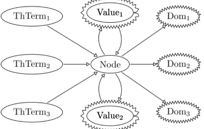
Node Value1 Value2 Value1 Value2 ThTerm2 ThTerm1 ThTerm3 Dom2 Dom1 Dom3
Figure 1: Relations between the object in the Egraph
Equivalence class information Informa-tion about each equivalence class can be recorded by an Egraph (e.g., at the root of the tree implementing the class in the union-find structure). It can be useful to record: a value v if the equivalence class contains v
as a node;
if not, a domain of feasible values that can be assigned to the theory terms in the class; a syntactic term in the equivalence class, if there is one (it can be useful if a representa-tive of the class is needed that is expressed in the vanilla first-order term grammar); if not, a theory term that can be picked as
the class representative.
In fact, we may record for the class different values for different theory modules. Indeed, several modules may want to assign values to the theory terms in an equivalence class, if they share the sort of these terms but are using different kinds of values for that sort [3], e.g., theory T1 assigning t←3/4 and theory T2 assigning u←red, with t and u in the same class. Having
both assignments is not necessarily unsatisfiable: 3/4and red will only have to denote the same
element in a(T1∪T2)-model. For instance, T1could be LRA, with t and u being of sort Q (the
rationals), andT2 could be a theory whose signature involves this sort while the semantics of
its inhabitants is irrelevant (e.g., the sort of values in the theory of arrays): T2 is still allowed
to use an arbitrary range of values such as red for its own reasoning mechanics, and store them in the Egraph. The Egraph does maintain the invariant that one theory module can only have at most one of its values in an equivalence class; and if there is one, it makes it readily available in the class information structure.
Likewise, the Egraph allows each theory module to maintain its own domain for the feasible values of a class. In fact, this domain can even be implemented as a composite domain: for instance the theory of bitvectors may maintain, as in [13], a bitvector interval domain, e.g., [1010, 1110], together with a bitvector mask domain, e.g., 1??0. Values to be picked must be in the intersection of the domains; in this example 1010, 1100, and 1110 are feasible. Disequality information is also recorded as a domain for the class (indicating which other equivalence classes should not be merged with this one).
Egraph operations We now describe the operations that transform the Egraph during the model building phase; they each correspond to an exported primitive in the Egraph API. Any node participating to one of the Egraph operations must be registered. Until then the node is dormant; separating node creation and registration avoids reasoning on a part of formula that is not needed: e.g., with ite(c, t, e) the nodes t (resp. e) could be dormant until we know that c has value⊺ (resp. )). Four kinds of Egraph operations can be applied to an Egraph E: Merge: Two registered nodes n1 and n2 have their equivalence classes merged, the resulting
Egraph being denoted merge n1 n2in E.
ThTerms: The classes of a registered node and a theory term are merged.
Value: The value of a registered node is set, merging the classes of the node and the value. Domain: The domain of a registered node is set or modified.
Operation Value (resp. ThTerms) is not subsumed by Merge, because the value (resp. the theory term) does not have to be registered. Because of this, none of the four operations above increase the number of equivalence classes, even temporarily.
Daemon Constraint Programming as known in the CP community, uses domains extensively with the help of daemons also called suspension [1, p. 185]. Daemons specify on which events they are waiting (e.g., the domain of specific node is modified, two equivalence classes are merged). They also provide a call-back function, to be run when the daemon is woken. In our design, daemons can wait on the following events:
Domains: wake up when the specific kind of domain for a specific node is modified. We write(t ◁ED) when, in Egraph E, the theory term t has domain D in its class;
Values: wake up when the specified node gets a value of the specified kind in its class. We write(t←Ev) when, in Egraph E, the theory term t has value v in its class.
If on the contrary the class of t has no values of the specified kind we write(t /←E).
Node Registered: wake up when the specified node is registered;
Theory Terms Registered: wake up when a theory term of the specified kind is registered; Value Registered: wake up when a value of the specified kind is registered;
Repr: wake up when this node is no longer the representative of its equivalence class. The events Domains and Values could be used for example for Boolean or arithmetic propa-gation. The events Node Registered can be used when delaying the registration of a sub-term, to know that it has been registered from somewhere else. The events Theory Terms Regis-tered and Value RegisRegis-tered are used for initializing other daemons, for example to perfom domain or value propagations. The events Repr is used for congruence closure, as indeed for n≜ f(x) we should merge the theory term f(y) with n when x is not the representative anymore. Ordering The daemons are not woken immediately when an Egraph operation is performed. Otherwise a wake-up chain could be triggered, leading to potential loops or stack overflows. More importantly, this would make reasoning a lot harder. So most of the wake-ups are de-layed. Also a merge between two classes cannot be done before the domains of the two classes are merged and therefore identical. Some daemon must be run with a higher priority than merging, for example because they ensure some invariant of a domain (for example for keeping a normalized linear polynomial as a domain), we call these daemons impatient. In order to sat-isfy these constraints the Egraph processes the actions using different queues in the following order of preference:
1. The registration of a node is done immediately, the woken deamons are queued. 2. Modification of domain is done immediately, the woken deamons are queued.
3. Setting of a value is done immediately if it is not registered and the woken daemons are queued, otherwise the merging of the nodes is queued.
4. Setting of a theory term is done immediately if it is not registered and the woken daemons are queued, otherwise the merging of the nodes is queued.
5. Running of impatient daemons.
6. Merging domains of the nodes that are going to be merged
7. Finish the merging of the nodes and the woken daemons are queued. This queue has always at most one element.
8. Start the merge of a pair of nodes, marked as merging n1 n2 in E by expl. It is done
in two steps: first, queuing their domains, if different, for merging (priority 6); second, queuing the finishing of the merge (priority7).
9. Run the other daemons. 10. Run the decisions.
The last two queues could be handled by an external scheduler that also handles the back-track points and the alternation between the model building phase and conflict analysis phase.
Explanation Triggering most of the Egraph-transforming operations requires providing a piece of data called explanation. That data is later used during conflict analysis so as to remember why the operation was performed. The format of that data is specific to the module having triggered the operation, since the data will be passed back to the module if and when conflict analysis asks why this operation was performed. Explanations are similar to the theory proofs of [2]. Here, a particular case of explanation is the dummy one that marks the operation as having been performed “for no reason”, i.e., as a decision. Such unjustified operations will be potential points of backtrack during search, as discussed in the next paragraph. An explanation is required for the Merge, Value and ThTerms operations, but not for the Domain one. It is required for the former because the equality is a central notion that any theory could use. On the other hand, the latter is specific to the theory that maintains this domain. Nonetheless at any time an explanation can be stored on the trail; we will see an example of this in Section4.2.
Decisions During the model building phases, theory modules can declare their interest in some decisions being made (e.g., “I need the value of that variable to be decided”). The format of such declarations is again theory-specific, but it contains at least a declared Egraph node of interest. Such declarations are recorded centrally in a decision queue, which is a priority queue that uses the usual VSIDS heuristics [10], based here on the activity of nodes. When a clause is learnt, a set of useful nodes is identified in order to update their activity. When no more propagations are to be done, the scheduler selects one possible decision out of the decision queue, and asks the theory module that created it whether the decision is still needed. Indeed, since the proposed decision was placed into the queue, events might have happened (e.g., propagations) that make it obsolete. If the decision is not needed after all (e.g., the value of a variable has been already determined by propagation), the scheduler moves on without creating a backtrack point. If the decision is needed, the scheduler creates a backtrack point and applies the Egraph operation specified by the decision.
Conflict When a conflict is found by a daemon during propagation, the Egraph is notified and an explanation is given, this time justifying the conflict rather than a propagation. The Egraph could detect a conflict by itself when attempting an operation merge n1n2in E, e.g., if
n1←Ev1and n2←Ev2for two values v1and v2of some theoryT that are different. In that case
the merge is not performed (as we prefer to keep the Egraph in a sound state) and, accordingly, the explanation expl given for the failed operation merge n1n2 in E is not added to the trail.
Instead, it contributes to the explanation Diff value(expl, n1, v1, n2, v2) (c.f. Section4.1) that
the Egraph gives to justify the conflict that it detected. When the Egraph detects or is notified of a conflict, it in turn notifies the scheduler, which starts the conflict analysis phase. Conflict analysis computes the backtrack point that the scheduler should go back to, restoring the Egraph datastructure that existed then. The only information kept from this branch exploration is the constraint learnt during conflict analysis (and the VSIDS heuristic score updates). This ensures the Egraph does not grow indefinitely with the arbitrary values used during search.
3
Conflict Analysis
The conflict analysis phase should produce a new constraint that forbids at least the last decision that was made. In order to do that, explanations for Egraph operations are recorded in a trail, a stack that is similar to that used in CDCL, MCSAT and CDSAT. The number of elements in the trail is the current age. Backtrack points corresponds to particular ages of the stack.
Node history An additional structure, called the node history or nodehist, is used to answer the question: “are two nodes n1and n2in the same equivalence class, and if so, at which age did
they first appear in the same class?”. This is useful information because the trail has recorded, at this age, the explanation given for the merge. The node history, given a node n, indicates (i) at which age an this node stopped being the representative of its class and (ii) what its new
representative newrep(n) was. Recording that information during the model building phase is done in constant time. To answer the above question during conflict analysis, assume without loss of generality that an1 < an2; then if newrep(n1) is n2 the answer to the question is an1,
and otherwise the answer is recursively computed for newrep(n1) and n2.
Hypotheses and split function The conflict analysis is similar to that in other frameworks such as CDCL, MCSAT or CDSAT. It starts when a conflict is notified to the Egraph. The
analysis maintains a conflict, i.e., a list H1, . . . , Hn of conflict elements or hypotheses such that
H1, . . . , Hn ⊧T∞ , where T∞ is the union of the combined theories, as in [3]. Hypotheses are
theory-specific and calledT -hypotheses; each T -hypothesis H should hold in the partial model described by the Egraph E, i.e., E⊧T H (in [3] the conflict elements had to be explicitly present
in the trail; here it can hold in a less direct way). The theory module forT must provide a means to retrieve, from H, the reasons why it holds according to the current Egraph E. Technically, this is given as a set ages(H) of ages, identifying the Egraph operations that contribute to making H hold. For instance an LRA-hypothesis H could be (0 ≤ x + y); assuming that H holds according to the Egraph E because x←E2 and y←E3, we would have ages(H) = {ax, ay},
where ax(resp. ay) is the age when x and 2 (resp. y and 3) first appeared in the same class.
The analysis starts with H0 ⊧T∞ and H0 = . Then each step consists of replacing one
hypothesis H by a set of hypotheses such that H1, . . . , Hn⊧T∞H, as in [3] again. We use the
ages of hypotheses in the same way a SAT solver uses the levels of literals in a conflict clause: the maximum agemax(H) of the set ages(H) is greater than or equal to the age of the last
decision, if and only if hypothesis H belongs to the level of the conflict; then
If only one hypothesis in the conflict belongs to the level of the conflict, it forms a UIP and we can stop conflict analysis;
Otherwise the hypothesis H with greatest agemax(H) is chosen for replacement. The
re-placement is done by looking up, in the trail, the explanation that was given for the Egraph operation performed at age agemax(H), and use that to recover new hypotheses H1, . . . , Hn
such that H1, . . . , Hn⊧T∞H.
We now look at how the new hypotheses H1, . . . , Hn are recovered. If H is aT1-hypothesis,
the theory module forT1 can provide agemax(H). Typically, the explanation expl found in the
trail at age agemax(H) is the explanation of a merge (merge n1n2 in E), which was triggered
by the theory module for a theoryT2. From a logical point of view, we have E∧(n1=n2) ⊧T1 H
and therefore E⊧T1 (n1=n2) ⇒ H. We then rely on the T1 theory module to provide newT1
-hypotheses H1, . . . , Hk, denoted splitT1(H, n1, n2), that form an interpolant between E and
(n1=n2) ⇒ H, in the sense that E ⊧T1 H1∧ ⋅ ⋅ ⋅ ∧ Hk and H1, . . . , Hk⊧T1(n1=n2) ⇒ H.
For example, assume thatT1is the theory of pure equality,T1-hypotheses are just equalities,
H is x=y, and H holds in E because there is in E a chain of equalities, a.k.a. equality path, from x to y. If the equality that was last added to the chain is a= b, then agemax(H) is the age of the merge between the classes of a and b, and splitT1(H, a, b) is the set of T1-hypotheses
{(x=a), (b=y)}. More interestingly, if T1 is LRA and 0≤ x + y holds in the partial model E
because x←E2 and y←E3, splitLRA(0 ≤ x+y, a, b) is the set of hypotheses {(0 ≤ b+y), (x=a)}
if a= b is on the equality path from x to 2, and {(0 ≤ x + b), (y=a)} if it is on the equality path from y to 3. This is reminiscent of the substitution mechanism of [6], used during conflict analysis when the last operation that contributed to the conflict was a propagated assignment. Then the theory module for T2 can use splitT1(H, n1, n2) to produce H1, . . . , Hn such
that H1, . . . , Hn ⊧T∞H. Typically, it will add to splitT1(H, n1, n2) = {H1, . . . , Hk} some T2
-hypotheses Hk+1, . . . , Hn that entail n1=n2 and that can be recovered from the explanation
expl recorded for the merge(merge n1n2 in E). Unless that merge was a decision, n1=n2 is a
consequence of E, and Hk+1, . . . , Hn will capture “what it is about E that justifies the merge”.
If the merge was a decision,{Hk+1, . . . , Hn} can simply be {n1=n2} itself, but in that case the
hypothesis n1=n2 is marked so that it is never picked for replacement in the next steps of the
conflict analysis (if the set{H1, . . . , Hn} replacing H contained H, conflict analysis would loop).
More generally, the production of H1, . . . , Hn according to each form expl can take is
de-scribed by conflict analysis rules, as illustrated in the next section with different examples of theoriesT2. Finally, the conflict analysis step replaces H by H1, . . . , Hn in the conflict.
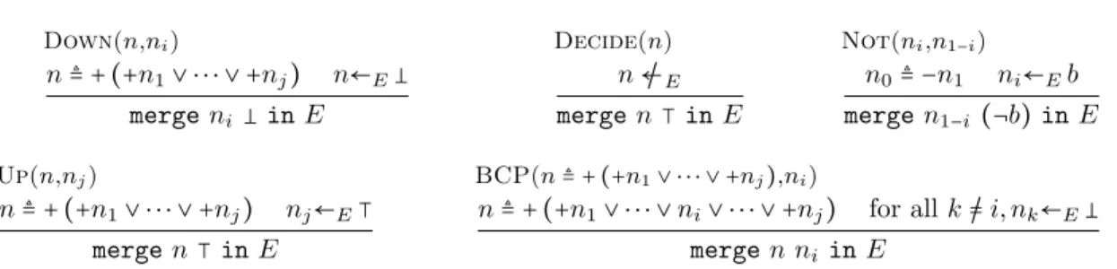
Down(n,ni) n≜ + (+n1∨ ⋅ ⋅ ⋅ ∨ +nj) n←E merge ni in E Decide(n) n /←E merge n⊺ in E Not(ni,n1−i) n0≜ −n1 ni←Eb merge n1−i(¬b) in E Up(n,nj) n≜ + (+n1∨ ⋅ ⋅ ⋅ ∨ +nj) nj←E⊺ merge n⊺ in E BCP(n ≜ + (+n1∨ ⋅ ⋅ ⋅ ∨ +nj),ni) n≜ + (+n1∨ ⋅ ⋅ ⋅ ∨ ni∨ ⋅ ⋅ ⋅ ∨ +nj) for all k /= i, nk←E merge n ni in E
Figure 2: Boolean Theory rules for the model building phase (simplified version only the + case of ± is shown). The name of the rules (Down, Decide, Not, Up, BCP –for Boolean Constraint Propagation, as in SAT) are the name of the explanations. The argument of the names are the information kept for the analysis phase.
Down(n,ni) H split(H, ni,) n = Decide(n) H split(H, n, ⊺) n = ⊺ Not(n,n′) H split(H, n′ ,(¬b)) b = n Up(n,nj) H split(H, n, ⊺) nj= ⊺ BCP(n ≜ + (+n1∨ ⋅ ⋅ ⋅ ∨ +nj),ni) H
split(H, n, ni) for all k /= i, nk =
Figure 3: Boolean Theory Conflict Analysis (simplified version). Each rule corresponds to the analysis of the propagation rule of the same name in Figure2
.
Value contradiction The conflict explanation given when merge n1 n2 in E fails because
of a clash of values between v1 and v2 is Diff value(expl, n1, v1, n2, v2). Its conflict analysis
inference rule replaces by analyze(expl, v1= v2). The analysis of expl will usually split the
equality into v1= n1 and n2= v2 and add the hypothesis used for propagating n1= n2.
4
Examples
4.1
Boolean
As in MCSAT and CDSAT, the Boolean theory does not use a CNF transform, and conjunctions and disjunctions could be arbitrarily nested. But the implementation still uses a two-watched literals mechanism to implement Boolean Constraint Propagation (BCP). Theory terms are of the form n≜ ± (±n1∨ ⋅ ⋅ ⋅ ∨ ±nj), as described previously. This format can represent conjunctions
and disjunctions, and importantly it reduces the need to create nodes that are just negations of each other. The values are⊺, and there are no domains used for that theory.
Figure2shows the propagation rules: the premises of each rule are events that the theory’s daemons are notified about, and the conclusion is the Egraph operation that is triggered. The name of the rule and its parameter form the explanation given to the Egraph, i.e., the information kept for the conflict analysis phase. For readability, only the cases when± is + are
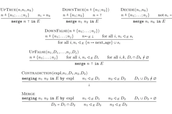
UpTrue(n,ni,nk) n ≜ {n1; . . . ; nj} ni=nk merge n ⊺ in E DownTrue(n ≜ {n1; n2}) n ≜ {n1; n2} n = ⊺ merge n1 n2 in E Decide(ni,nk) n ≜ {n1; . . . ; nj} not ni=nk merge ninkin E DownFalse(n ≜ {n1; . . . ; nj}) n ≜ {n1; . . . ; nj} n←E for all i, ni◁Esi
for all i, ni◁E{n ↦ next age} ∪ si
UpFalse(n1,D1,. . . ,nj,Dj)
n ≜ {n1; . . . ; nj} for all i, ni◁EDi for all i, k, Di∩Dk= ∅/ merge n ⊺ in E Contradiction(expl,n1,D1,n2,D2) merging n1 n2 in E by expl n1◁ED1 n2◁ED2 D1∪D2= ∅/ Merge merging n1 n2 in E by expl n1◁ED1 n2◁ED2 D1∪D2= ∅ D3=D1∩D2 n1◁ED3 n2◁ED3
Figure 4: Equality Theory Propagation
shown; the other cases can be obtained by switching⊺ and according to whether ± is + or -. The rules of figure3are the conflict analysis inference rules as described in Section3: there is one rule for each kind of explanation, which is indicated again in the rule name. The premise of the rule is the hypothesis H (from another theoryT ) that needs replacing, and the conclusion of the rule is the set of new hypotheses that H is replaced with. As mentioned in Section 3, the rules rely on the function splitT1 provided byT1, abbreviated as split in the figure.
n5 ³¹¹¹¹¹¹¹¹¹¹¹¹¹¹¹¹¹¹¹¹¹¹¹¹¹¹¹¹¹¹¹¹¹¹¹¹¹¹¹¹¹·¹¹¹¹¹¹¹¹¹¹¹¹¹¹¹¹¹¹¹¹¹¹¹¹¹¹¹¹¹¹¹¹¹¹¹¹¹¹¹¹¹µ n1∧ (n2∨ −n3) ´¹¹¹¹¹¹¹¹¹¹¹¹¹¹¹¹¹¹¹¹¹¹¹¸¹¹¹¹¹¹¹¹¹¹¹¹¹¹¹¹¹¹¹¹¹¹¶ n4 ∨ n7 ³¹¹¹¹¹¹¹¹¹·¹¹¹¹¹¹¹¹¹µ n5∨ n6 n8 ³¹¹¹¹¹¹¹¹¹¹¹¹¹¹¹¹¹¹¹¹·¹¹¹¹¹¹¹¹¹¹¹¹¹¹¹¹¹¹¹¹µ −n2∨ −n1
We are illustrating the boolean propaga-tion and learning with an example wich is not in CNF (n1∧ n4 is used as a shorthand
for −(−n1∨ −n4)), n7 and n8 are set to ⊺
at level 0. A sequence of decision and propagation gives the trail: Decide(n3), BCP(n4 ≜
+(+n2 ∨ −n3), n3), Decide(n1), BCP(n1 ≜ n1 ∧ n4, n1) and leads to the contradiction
Diff value(BCP(n8 ≜ +(−n2 ∨ −n1), n1), n1,⊺, n8,). The conflict analysis start with
H0 ≜ ⊺ = , then H0 is replaced by (H1 ≜ ⊺ = n1), (H2 ≜ n2 = ⊺), (H3 ≜ n8 = ), then H2
is replaced by(H4≜ n2= n4), (H5≜ n7= ⊺), H1 which leads to the new constraints¬H1∨ ¬H4
(H3 and H5 have a level before the first decision).
4.2
Equalities
The theory of equality is responsible for the equality symbol but also of the n-ary function distinct. So theory terms are of the form m ≜ {n1; . . . ; nj}, which intuitively stands for
⋁i⋁k,k /=ini= nk. When this theory term is false we directly have the semantics of distinct.
The implementation efficiently implements the distinct symbol by (i) tagging all arguments of distinct (when it has the⊺ value) with the same tag (the node m), and (ii) checking that no merging is done between nodes sharing the same tags. For each node we store the set of tags
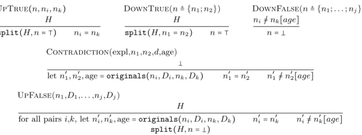
UpTrue(n, ni, nk) H split(H, n = ⊺) ni=nk DownTrue(n ≜ {n1; n2}) H split(H, n1=n2) n = ⊺ DownFalse(n ≜ {n1; . . . ; nj}) ni=/nk[age] n = Contradiction(expl,n1,n2,d,age) let n′ 1, n ′ 2, age = originals(ni, Di, nk, Dk) n′1=n′2 n ′ 1=/n′2[age] UpFalse(n1,D1,. . . ,nj,Dj) H for all pairs i,k, let n′
i, n ′ k, age = originals(ni, Di, nk, Dk) n′i=n′k n ′ i=/n′k[age] split(H, n = )
Figure 5: Equality Theory Conflict Analysis
m1, . . . , mlas a domain: {m1↦ age1; . . . ; ml↦ agel}. The age1, . . . , agelare the age of the trail
when the corresponding tag was added. The propagation rules are shown in Fig.4, where n◁ED
means that n has domain D in the Egraph E. Even if DownFalse is not a merge we require the explanation to be added to the trail (at age next age). Merge is not added to the trail because it does not add any information. Fig.5shows the conflict analysis rules. Hypotheses H are of the form n1/= n2[age], which is interpreted as a disequality and where ages(H) = {age}.
The function originals(n1, D1, n2, D2) computes the origin of a disequality, i.e. the two nodes
and the age at which the nodes have been made disequal. Formally, originals(n1, D1, n2, D2)
computes from n1, n2 and two non-disjoint sets of tags D1, D2, the nodes n′1, n′2 and age such
that it exists m≜ {n′ 1, n
′
2, . . .}, m ↦ age ∈ D1∪ D2 and n1 (resp. n2) have been merged with n′1
(resp n′
2). The node history allows to know what has been merged.
5
Conclusion
The concepts and the prototype described in this paper can be further developed and extended to other theories, but we hope the initial development illustrates how an Egraph and domains could form useful features of an MCSAT implementation. We would like to thanks Simon Cruanes for his participation to fruitful discussions.
References
[1] A. Aggoun et al. Eclipse user manual release 5.10. 2006.
[2] M. P. Bonacina, S. Graham-Lengrand, and N. Shankar. “Proofs in Conflict-Driven Theory Combination”. In: Proc. of the 7th Int. Conf. on Certified Programs and Proofs (CPP’18). 2018.
[3] M. P. Bonacina, S. Graham-Lengrand, and N. Shankar. “Satisfiability Modulo Theories and Assignments”. In: Proc. of the 26th Int. Conf. on Automated Deduction (CADE’17). Vol. 10395. 2017.
[4] S. Conchon et al. “CC(X): Semantic Combination of Congruence Closure with Solvable Theories”. In: ENTCS 198.2 (2008).
[5] S. Graham-Lengrand and D. Jovanovi´c. “An MCSAT treatment of Bit-Vectors”. In: 15 Int. Work. on Satisfiability Modulo Theories (SMT 2017). 2017.
[6] D. Jovanovi´c. “Solving Nonlinear Integer Arithmetic with MCSAT”. In: Proc. of the 18th Int. Conf. on Verification, Model Checking, and Abstract Interpretation (VMCAI’17). Vol. 10145. 2017.
[7] D. Jovanovi´c, C. Barrett, and L. de Moura. “The Design and Implementation of the Model Constructing Satisfiability Calculus”. In: Proceedings of 13th International Conference on Formal Methods in Computer-Aided Design, FMCAD 2013. 2013.
[8] D. Jovanovi´c and L. de Moura. “Solving non-linear arithmetic”. In: IJCAR 2012. [9] B. Mishra and P. Pedersen. “Arithmetic with real algebraic numbers is in NC”. In:
Pro-ceedings of the international symposium on Symbolic and algebraic computation. ACM. 1990.
[10] M. W. Moskewicz et al. “Chaff: Engineering an Efficient SAT Solver”. In: DAC. 2001. [11] L. de Moura and D. Jovanovi´c. “A Model-Constructing Satisfiability Calculus”. In:
VM-CAI 2013.
[12] G. Nelson and D. C. Oppen. “Simplification by cooperating decision procedures”. In: ACM Transactions on Programming Languages and Systems (TOPLAS) 1.2 (1979).
[13] A. Zeljic, C. M. Wintersteiger, and P. R¨ummer. “Deciding Bit-Vector Formulas with mcSAT”. In: Proc. of the 19th Int. Conf. on Theory and Applications of Satisfiability Testing (RTA’06). Vol. 9710. 2016.