Cycle to cycle feedback control of manufacturing processes

Cycle to Cycle Feedback Control

of

Manufacturing Processes

by

Tsz-Sin Siu

University of Toronto, 1999

Submitted to the Department of Mechanical Engineering in Partial Fulfillment of the Requirements for the Degree of

Master of Science in Mechanical Engineering

at the

Massachusetts Institute of Technology

February 2001

C2001 Massachusetts Institute of Technology All rights reserved

Signature of Author ... Certified by ... MASSACHUSETTS

INSTIMU

JUL 16 2001

LIBRARIES

Depktment of Mechanical Engineering January 29, 2001

.-... David E. Hardt Professor of Mechanical Engineering Thesis Supervisor

0

Accepted by ... --

...---Ain A. Sonin Chairman, Department Committee on Graduate Students

Cycle to Cycle Feedback Control

of

Manufacturing Processes

Tsz-Sin Siu

Submitted to the Department of Mechanical Engineering on January 29, 2001 in Partial Fulfillment of the Requirements for the

Degree of Master of Science in Mechanical Engineering

Abstract

A new concept of process control in manufacturing called Cycle-to-Cycle (CTC) feedback control is introduced in this research. It is done by applying feedback from the final output of a

manufacturing process, using the information from the current cycle to improve quality for the following cycles. Run-by-Run (RbR) control in semiconductor industry is found to use a similar idea of discrete feedback control. CTC control will be a complement to existing RbR technologies by presenting a stronger emphasis on control theory and expanding the application to other manufacturing processes.

Models for different process components are presented for CTC systems. Theories of discrete control system are used for analysis. Proportional and integral controls for CTC systems are analyzed using a linear process gain model with additive disturbance.

Two manufacturing processes -metal bending and injection molding -are carried out to demonstrate the advantages of CTC control and also to verify the accuracy of the models. As predicted, we found that CTC control can increase variation on uncorrelated process such as metal bending and reduce variation on correlated processes such as injection molding. Even for

uncorrelated processes, however, CTC control can be used to reject common disturbances and bring the process closer to the desired target. As a result, CTC control is able to improve overall process capability by either reducing the variance or by removing the mean shift from the target.

It is shown experimentally that the linear additive models of the process and the disturbance are accurate. Analytical and graphical tools are very useful in predicting behavior of actual systems. It is also shown in the experiments that an optimization technique, which is based on the

minimization of mean squared error, is effective in designing an optimal controller for the metal bending process.

Thesis Supervisor: David E. Hardt

Title: Professor of Mechanical Engineering

Acknowledgements

Achieving success in life is about achieving equilibrium. During my stay here at MIT, I learned to reach the state of equilibrium that had transformed me into a different person. I achieved that balance with the guidance of people around me (or engineers would call it "feedback"). I met more people from different background than ever before. I learned to share and give.

I would like to sincerely thank my research advisor, Professor David Hardt, for his ample and enthusiastic support for this research, and particularly his timely motivations that constantly re-energized my interest during the course of the project. Although my stay here at MIT has been

quite short, your influence on me would certainly last for the rest of my life. Thanks also to SMA (Singapore-MIT Alliance) for generously providing the funding for this project. Thank you Gerry, Dave, Bob and Mark in the machine shop for helping me on the experiments during this project.

Everyone in the research group help made this thesis possible. Lisa helped with all the

administrative stuff. Walt helped share my worries about job search. John showed me how to learn and think scientifically and rationally. Benny kept me up to date with new discovery on literatures.

To my father Bun-Wing, my mother Ching and my brother Peter for their support. I certainly miss the times I stayed at home but my encounter at MIT helped develop myself to be a complete person.

My roommate Kai is always pessimistic about life. I know you had a roller coaster experience here, but at least you made it and got a decent job earlier than any one of us. I hope you will learn to be optimistic and enjoy your work in California. Josh provides the daily dose of lunchtime relief and thanks for sharing a lot of interesting stories. Chee Wei is a lucky man, I wish Maggie and you the

best. Keng Hui is a smart and witty guy, and I hope your generosity will lead you far and high in your career. Allen is full of surprises, and Saturday Haymarket trips are definitely the most

memorable experience. Winston is most organized person that I have ever met, and by chance he is also a Canadian. Thank you for teaching me how to stay on my goals. Thank you Ceani for helping me to find the job at graduate admissions so I could get through my studies smoothly. Rhonda helped me solve a lot of problems while I was finishing this research. Well Ada, I don't know where to mention you, but thank you for being a close friend for more than 8 years.

I want to say thanks to Simon, Federico, Rogelio, Andrew, Shivanshu, Sascha, Yogesh, Carlos, and Cesar for sharing memorable moments with me Thank you for teaching me things in life. Thanks to all my friends in Mechanical Engineering, especially those in the LMP, for their everyday support that allows me to overcome all the hurdles.

Before I started my studies here at MIT, Professor Ely Sachs told me that I would work harder than I have ever worked before. It certainly lived up to his comment. Thank you for helping me reach my potential. I also learned to enjoy life, as we all only live once and work is only part of life. Keeping a balance life not only enhances my efficiency at work, it also may research work more enjoyable and meaningful. Thank you Professor Sanjay Sarma for providing the comic relief during the stressful days as a teaching assistant; and you still owe me a coffee. And to all the students in the class, good luck in your future endeavor.

Quite unexpected for my stay here at MIT, I met a lot of people outside the academic circle. For my job as a database consultant, I got to meet a lot of people that assist the administration of the institution. I certainly learned a lot through the experience. It expanded my views and

understanding of the cultures, history, religion and politics by interacting with different people all around the campus. Marina, Bette, Elizabeth, Linda, Monica and Tammy at the graduate

admissions office especially gave me the care and guided me through my toughest times. They deserve my deepest gratitude as a pupil and friend.

MIT is a place that affects people. Through its rich culture of academics and research, it attracts the brightest and the most passionate scholars from around the world. President Vest calls MIT a learning institute. Whether it is an undergraduate student taking an introductory course to fulfill a degree requirement or a post-doctoral associate conducting cutting edge research trying to push the envelope of existing knowledge, we all have a common goal. The goal is to investigate and learn the truth about the natural and the artificial in a rational and scientific manner. What distinguishes MIT from other schools is not the course material being taught in classes, but rather the deep heritage that it embodies. At MIT, people work diligently to be the leaders of tomorrow; people work hard to achieve what they want; and people work endlessly to change the world. I am lucky to try to be one of them. So last but certainly not least, I must thank MIT for giving me the

opportunity to learn with you, and to achieve some of the goals that I would never have achieved elsewhere.

Table of Contents

Abstract ...

3

A cknow ledgem ents ...

5

Table of Contents ...

7

List of Figures ...

11

List of Tables...

13

Glossary...

15

Chapter 1: Introduction

...

17

1.1. D efinition of Quality ...

17

1.2. Conventional M ethods of Quality Control...

18

1.2.1. Acceptance Sampling ... 18

1.2.2. Statistical Process Control and its notion of feedback ... 19

1.3. Autom atic Feedback Control ...

20

1.3.1. Cycle-to-cycle feedback control... 20

1.3.2. Difference between CTC control and machine control... 21

1.4. Research Goals...

23

1.4.1. Discrete control tools for CTC control... 24

1.4.2. Experiments of CTC control on new processes ... 24

1.5. Expected Reader Background and Thesis Outline...

24

Chapter 2: Literature Revie

27

2..

Pier...27I

.h

2.1.1. Box and Kramer ... 27

2.1.2. Sachs, Hu and Ingolfsson ... 29

2.1.3. Vander W iel and Tucker ... 31

2.2. M ore Recent D evelopm ents... 32

2.2.1. T. Sm ith and D. Boning... 32

2.2.2. Del Castillo and Hurwitz... 32

2.2.3. Del Castillo... 33

2.2.4. Valjavec and Hardt... 33

2.3. The Future ...

34

2.3.1. The Next-Generation M anufacturing Project... 34

2.4. M otivation for Cycle-to-Cycle feedback control ... 35

Chapter 3: Theoretical Background

37

3.1. Cycle-to-Cycle System M odels... 37

3.1.1. Process and Disturbance models ... 37

3.1.2. Delay models... 39

3.2. D iscrete Control System Analysis ... 40

3.2.1. Z-transform and analysis... 40

3.2.2. Adding Randomness to the system ... 42

3.3. Characterizing Cycle-to-Cycle Control System s ... 42

3.3.1. Root locus diagram in Z-plane... 42

3.3.2. Steady-state error analysis ... 43

3.3.3. Settling time analysis ... 45

3.4. Analysis of Cycle-to-Cycle Control Systems ...

45

3.4.1. Proportional control with direct feedback... 45

3.4.2. Integral control with direct feedback ... 50

3.5. Analysis Summary...55

Chapter 4: Design of Minimum Quality Loss Controller...57

4.1. Introduction to Controller Design...

57

4.2. Performance M easuring Techniques ...

58

4.2.1. Performance metrics used in Manufacturing Quality Control... 58

4.3. Cycle-to-Cycle feedback control scheme and its design criteria...59

4.3.1. Performance Metric of Cycle-to-Cycle feedback controller... 60

4.4. Optimal Controller Design for Cycle-to-Cycle Systems ...

62

4.5. Step disturbance example ...

63

Chapter 5: Application to Sheet Metal Bending Process... 69

5.1. Introduction...69

5.1.1. Manufacturing Process Taxonomy ... 69

5.1.2. Selection of appropriate processes for experimentation ... 70

5.1.3. Description of Air Bending process... ₇₁

5.1.4. Process Model and Assumptions ... 72

5.2. Experimental Setup...

73

5.2.1. Expected Results... ₇₅

5.3. Experimental Procedure and Observations...

76

5.4. Results and Analysis...78

5.4.1. Characterization of Process Gains ... 78

5.4.2. Open-loop Run... 80

5.4.3. Closed-loop with no deterministic disturbance... 81

5.4.4. Closed-loop with step disturbance (sudden shift of material properties)... 84

5.4.5. Closed-loop with ramp disturbance (gradual change of tailstock position)... 86

5.4.6. Optimally designed gain with material shift... 88

5.5. Conclusions...91

Chapter 6: Application to Injection Molding Processes... 93

6.1. Introduction...93

6.1.1. Description of Injection Molding Process ... 93

6.1.2. Process Model and Assumptions ... 95

6.2. Experimental Setup... ₉₆

6.3. Experimental Procedure and Observations... 99

6.3.1. Procedures... ₉₉

6.3.2 . O bservations ... 100

6.4. Data analysis...101

6.4.1. Design of experiment to characterize process gain... 101

6.4.3. Closed-loop control of the process with I-controller... 109

6.5.

Conclusions...

111

Chapter

7:

Conclusions and Recommendations... 113

7.1. Summ ary of results ...

113

7.1.1. Experimental results ... 113

7.1.2. Additional insights ... 114

7.2. Recomm ended future work...

115

7.2.1. Short-term research goals... 115

7.2.2. Long-term research goals ... 115

7.3. Final words...

116

Appendix

B

...

127

XR... 133

Bibliographical Note ...

136

List of Figures

Figure 1.1: Acceptance sampling implementation... 18

Figure 1.2: Classical Control System View of SPC implementation... 19

Figure 1.3: Cycle-to-cycle discrete-time control implementation ... 21

Figure 1.4: Material variations are outside the loop of machine state control... 22

Figure 1.5: Process control that includes material control... 22

Figure 1.6: Process control by feeding back critical output parameters ... 23

Figure 3.1: C ontrol system blocks ... 37

Figure 3.2: An appropriate process m odel... 38

Figure 3.3: A simple additive disturbance model ... 38

Figure 3.4: Pure process delay m odel... 39

Figure 3.5: Control Block Diagram for proportional controller... 41

Figure 3.6: A first order correlated disturbance ... 42

Figure 3.7: Comparison of root locus plot in s-plane (left) and z-plane (right)... 43

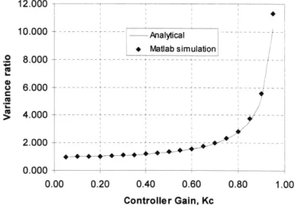
Figure 3.8: Matlab verification of the analytical result for a P-controller with NIDI disturbance... 48

Figure 3.9: Time dependence of variance amplification for P-controller ... 49

Figure 3.10: Matlab simulation result showing variance reduction for a P-controller... 50

Figure 3.11: Control Block Diagram for Integral Controller ... 50

Figure 3.12: Root locus plot for a closed-loop integral control system ... 51

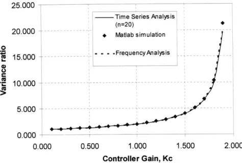
Figure 3.13: Matlab verification of the analytical result for I- controller with NIDI disturbance ... 53

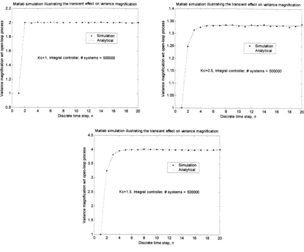
Figure 3.14: Time dependence of variance amplification for I-controller... 54

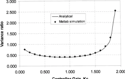
Figure 3.15: Matlab and frequency analysis results showing variance reduction for I-controller... 55

Figure 4.1: Discrete-time feedback implementation of a P-controller with random disturbance .... 60

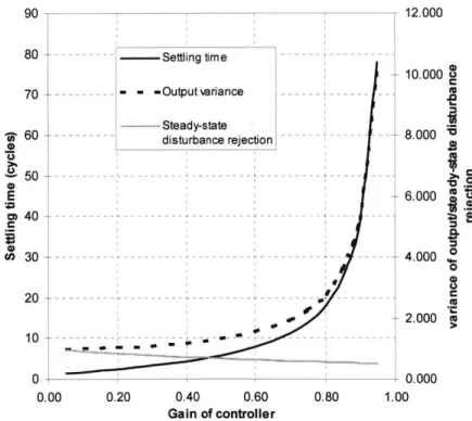
Figure 4.2: Variation of performance parameters for a P-controller with random disturbance ... 61

Figure 4.3: The two types of disturbances:... 63

Figure 4.4: Block diagram of a feedback control system with an I-controller on a shifted process 64 Figure 4.5: Control block diagram for a PI-controller ... 66

Figure 4.6: Root locus diagram for a PI-controller (with K=1, so the open-loop zero is at 0.5) ... 67

Figure 5.1: Manufacturing Process Taxanomy ... 69

Figure 5.2: Illustration of Air Bending Process ... 71

Figure 5.3: Model Schematics for Air Bending Process... 72

Figure 5.4: Setup for the metal air bending experiment on a lathe ... 73

Figure 5.5: Punch depth control using the precision dial on a lathe ... 74

Figure 5.6: A Vernier Protractor measuring part angle ... 75

Figure 5.7: Steps showing different bend angles at different punch depths... 76

Figure 5.8: Feedback Control schematics for air bending process... 77

Figure 5.9: Simulated deterministic output using optimal feedback gain ... 88

Figure 5.10: Performance Index minimization by K... 89

Figure 6.1: Illustration of Injection Molding Process... 94

Figure 6.2: Model Schematics for Injection Molding Process ... 95

Figure 6.3: Injection Molding Machine used for experiment... 96

Figure 6.4: Injection Molding Machine controller panel ... 97

Figure 6.5: Injection Molding Die Close-up with Part... 97

Figure 6.6: Dial Caliper measuring an injection molded part ... 98

Figure 6.7: Output Part Dimension ... 98

Figure 6.8: Feedback Control schematics for Injection Molding process ... 100

Figure 6.9: Comparison of a good and bad part ... 101

Figure 6.10: Correlation plot between hot and cold measurement... 104

Figure 6.11: P-controller closed-loop run ... 105

Figure 6.12: Autocorrelation comparison between open-loop process ... 106

Figure 6.13: P-controller closed-loop run with gain change ... 107

Figure 6.14: Root locus diagram for P-controller... 108

Figure 6.15: Closed-loop P-controller target shifted... 109

Figure 6.16: I-controller closed-loop run ... 110

Figure 6.17: Root locus diagram for I-controller ... 111

Figure 6.18: Illustration of a thermoformed part... 112

List of Tables

Table 5.1: Results of Process Gain Characterization experiments... 79

Table 5.2: Results of open-loop run experiments ... 80

Table 5.3: Results from undisturbed closed-loop experiment with P-controller ... 82

Table 5.4: Results from undisturbed closed-loop experiment with I-controller ... 83

Table 5.5: Results from shifted closed-loop experiment ... 85

Table 5.6: Results from closed-loop experiment with ramp disturbance... 87

Table 5.7: Experimental result for Minimum Quality Loss I-controller design ... 90

Table 6.1: Input parameters and the range of operations ... 101

Table 6.2: Design of experiment input levels used ... 102

Table 6.3: First round ANOVA table... 102

Table 6.4: Second round design of experiment result... 103

Table 6.5: Run statistics for P-controller run... 105

Table 6.6: Run statistics for disturbed P-controller run ... 107

Table 6.7: Run statistics for P-controller with varying target... 109

Table 6.8: R un statistics for I-controller ... 110

Glossary

SPC - Statistical Process Control CTC control - Cycle-to-Cycle control

RbR control - Run-by-Run control NGM - Next-Generation Manufacturing

P-controller - Proportional controller

PI-controller - Proportional Integral controller I-controller - Integral controller

MSE - Minimum squared error ST controller - Self-tuning controller MISO - Multiple-Input Single-Output DOE - Design of Experiment

ANOVA - Analysis of Variance

Chapter 1: Introduction

This thesis is about expanding the traditional concept of quality control in manufacturing: using feedback from the output of a manufacturing process, measured after each process cycle, as a means of systematic quality improvement. We call this Cycle-to-Cycle (CTC) feedback control. In this chapter, we will summarize some of the quality control techniques that are commonly used in

industry today. We will show that in some of the traditional techniques, the notion of feedback control has long existed. The problem, however, lies on the fact that most of the control schemes are based on subjective operator judgments. We will also present the traditional use of in-process control in machine design to improve the process and how CTC feedback control can be

implemented to further improve the quality of the process.

1.1. Definition of Quality

In manufacturing processes, quality is how well the process output conforms to the design specifications. Output refers to the critical dimension or critical property of the output. In

machining, for example, the output is the critical dimension of the machined part and the accuracy of the machined part determines the quality of the output. In annealing process, the output is the average hardness of the annealed part and the quality is the uniformity of the hardness on the output part.

Quality is also defined as inversely proportional to variability [1]. Since variability can be

described only in statistical terms, statistical measures such as process capability' and quality loss2 are commonly used for quality improvement.

1.2. Conventional Methods of Quality Control

1.2.1. Acceptance Sampling

Acceptance sampling, also know as 100 percent inspection, is an end-of-pipeline solution to quality control. One can imagine this as a "quality filter" at the output of the process that only allows the acceptable parts to pass through. By inspecting every single output of the process, the quality of the products is guaranteed. Figure 1.1 shows how acceptance sampling is conducted.

Unscreened process output

Acceptance

ldffi

Sampling

0

Rework

Scrap

Figure 1.1: Acceptance sampling implementation

Source: DeVor [2, p. 28

Process capability, Cpk, is a statistical parameter commonly used to measure quality. It is defined as (USL -y p- LSL

Cpk = min , , where u and a-are the mean and standard deviation of the process, and

(3a '3

USL and LSL are the specification limits. A process with higher Cpk has better quality.

2 Quality loss, L, is usually a quadratic function describing the cost of being off target and is defined as

The advantage of acceptance sampling, obviously, is its 100% quality assurance. For mission critical parts that need to meet stringent quality requirements, acceptance sampling is the only way to guarantee complete compliance to specification. The disadvantages, on the other hand, are large quantities of wasted parts, lower production rate and high cost of inspection and rework.

Although acceptance sampling guarantees the quality of the output, it does not improve the process itself. The variability of the process output is still high, and this limits the process capability of the process.

1.2.2. Statistical Process Control and its notion of feedback

Statistical Process Control (SPC) is probably one of the most widely used techniques in quality control today. Samples of the process output are obtained and the collected data are usually

averaged (like a low pass filter) and plotted on a graph called a run chart. If a sample point is found to lie outside the process limits (usually ±3 a from the true mean of the process, where a is the standard deviation of the process), an alarm is signaled. The operator would then check for

anomalies in the machine, the material or the process itself and see if adjustments are needed. SPC allows the detection of assignable or special causes such as tool wear, material changes or human errors. Figure 1.2 below shows the feedback loop of SPC methodology.

T*

Process

Implementation Observation

Take action Data collection

Decision Diagnosis Evaluation

Formulate action Fault discovery Data analysis

Figure 1.2: Classical Control System View of SPC implementation

Source: DeVor [2], p. 134

Advantages of SPC include lower cost on inspection and rework, higher quality than without inspection, and lower waste than acceptance sampling. Its ability to signal critical problems in machine, material and operating procedure is also an important advantage. Compared to acceptance sampling, however, SPC does not have 100% quality assurance. Slow response to disturbances in input parameters due to the averaging effect is also a disadvantage.

In SPC, the goal is to maintain the output within the 3 a-limits. Quality control is a task performed by human decision. The control action can be inconsistent and arbitrary, so the variability is still high and the process capability limited.

1.3. Automatic Feedback Control

As seen in Figure 1.2, SPC uses the notion of feedback in quality control. The feedback signal, however, is only being used as a monitoring tool as opposed to a decision tool. In other words, SPC does not provide the user with a specific direction to improve the process. The ability to improve the performance of a process relies completely on the operator or production engineer's knowledge and experience. It is desirable, therefore, to devise an autonomous feedback control scheme that would automatically and intelligently fine tune the manufacturing process to achieve optimal performance.

For continuous processes, feedback control theory in the continuous domain can be applied to achieve desired dynamic behavior. For discrete part manufacturing, similar continuous feedback control can be used for the time period within each process cycle (herein referred to as "in-process" control). The final output, however, cannot be obtained until the discrete process cycle is complete. Our interest is in investigating the use of discrete control theory on data obtained after each process cycle, hereafter referred to as CTC feedback control.

1.3.1. Cycle-to-cycle feedback control

Cycle-to-cycle feedback control is the focus of this research. It can be thought of as a combination of acceptance sampling and automatic feedback control. In acceptance sampling, all output parts are sampled for quality assurance. By contrast, CTC control feeds back the information acquired

ControllerPrc

Control action

Cycle-to-Cycle Feedback Data collection and analysis

Figure 1.3: Cycle-to-cycle discrete-time control implementation

The obvious advantages of CTC control include a systematic control strategy that does not require subjective human decision-making and predictable performance based on theory. The

disadvantages of CTC control are the cost of measurement and the inability to diagnose assignable causes in the process. In order to popularize the use of CTC control, some of these disadvantages need to be overcome.

1.3.2. Difference between CTC control and machine control

Another way to look at CTC control is from a machine control point of view. One might ask what is the difference between traditional machine control and the proposed CTC control. Most high volume machines have sophisticated controllers to maintain machine parameters such as position, flow rate, pressure and temperature. But these controllers only control the machine states. The most important attribute of a process is its output, which can only be indirectly controlled by these machine state controllers. In addition, imperfection in the modeling of the relationship between machine parameters and the output can lead to output errors.

Variation in material properties is also a major cause of error on the output; and machine state control cannot possibly adjust for the variation in the material because material is out of the loop of machine state control (Figure 1.4 shows why machine state control cannot control material

variation). We can see that both the machine and material have variations in their property (stiffness, yield stress, melting point) and state (temperature, internal stress, shape). Machine state

control only compensates for the machine part of the process and thus leaves the variation of the output dependent on material variation.

Target + Controller Ma

me

Machine state feedback control

Figure 1.4: Material variations are outside the loop of machine state control

Source: Hardt [3]

A natural step to tackle this problem is to impose control on the material. Figure 1.5 below shows the control model that includes material control as well. It can be observed that this type of control still does not control the output directly. Because the interactions between the machine and the material can be unpredictable, the output variation is still high.

Target +

Controller

Ma

ine

Ma

rial

-

Output

Machine state feedback control

Material feedback control

Figure 1.5: Process control that includes material control

Source: Hardt [3]

To achieve direct control on the output, measurements of critical output parameters have to be obtained and fed back for adjustment. As shown in Figure 1.6, output feedback considers variations imposed by both the machine and the materials. We could, of course, implement machine state control and material control in conjunction with critical output control to reduce the amplitude of adjustment in the outer loop.

Target +

Controller

Maeine

Ma

i a

Output

Critical output feedback

Figure 1.6: Process control by feeding back critical output parameters

Source: Hardt [3]

In certain manufacturing processes such as chemical mixing, direct output feedback control can be achieved within the manufacturing cycle so the output can be controlled precisely for each

individual cycle. In most other cases, however, the critical output parameter (typically a dimension) will not be accessible until the manufacturing cycle is finished; by which time the current output,

even if out of specification, cannot be changed anymore. Cycle-to-cycle control is the use of this final output to adjust the proper input parameter for the following cycle. Cycle-to-cycle control is, therefore, discrete in nature and it can be applied to batch continuous processes and discrete parts manufacturing.

1.4. Research Goals

We started this research believing that CTC control would be a breakthrough in quality control. It was a subtle but important improvement towards conventional SPC scheme. As will be shown in chapter 2, it is found that substantial research had been done in the development of similar quality control scheme for semiconductor manufacturing. In reading through this literature, it was found that most of the theoretical development had been conducted from a statistical point of view. Some of the analyses were long and tedious; and more importantly, most of the theories lacked simple graphical design tools that are familiar to control engineers. The complexity of the statistics can be a hindrance in the widespread used of CTC control.

1.4.1. Discrete control tools for CTC control

The theories of discrete control have been in existent for a long time. In areas such as discrete signal processing, digital communications and digital control system, applications of the theories are diverse and comprehensive. Tools such as z-transformation and root locus plot on a unit circle can greatly ease the analysis and design process. We will bring some of these tools to CTC control and show examples of effective application.

1.4.2. Experiments of CTC control on new processes

Two applications of CTC control are carried out to verify analytical results and to demonstrate the use of design tools to predict system behavior. The three-point bending or air bending process represents a family of processes that has uncorrelated disturbances. It also has regular shifts or ramps that are somewhat predictable. In short run manufacturing situations, we could effectively use CTC control tools to optimally improve the process capability.

The injection molding process, on the other hand, has highly correlated disturbances. It represents a family of thermal processes that can take benefit of the variance reduction capability of CTC control.

1.5. Expected Reader Background and Thesis Outline

In order to take full advantage of the discussions in this thesis, it is expected that the reader be familiar with classical feedback control theory, elementary statistics, manufacturing processes and some knowledge on difference equations and matrix operations.

This thesis highlights the two main focuses of the research of CTC feedback control: theoretical development and application by experimentation. One who is familiar with run-by-run control can skim through chapter 2 and focus more on the discrete control theories presented in chapters 3 and 4. Those who are familiar with discrete stochastic control theory may elect to skip chapter 3.

stochastic control theory, with short run manufacturing and correlated disturbances some of the important themes. Chapter 2 presents a thorough review of the history of CTC feedback control and summarizes the current state-of-the-art of the field. It also seeks to define a vision on which CTC feedback control can be integrated into manufacturing equipment design in the future. The essential theoretical background of the CTC feedback control, which is extracted from discrete feedback control, is presented in chapter 3. Several graphical and analytical tools for discrete feedback control are also presented.

Chapter 4 contains an analytical framework for designing minimum quality loss controller and the method is later used in the air bending process to illustrate the concepts.

Applying the theory to existing manufacturing processes is a non-trivial task and the advantage of CTC may not be immediately appealing to engineers or managers. Chapter 5 deals with the appropriate application of CTC feedback control to manufacturing processes. Common

manufacturing processes are categorized. Chapters 5 and 6 also contain experimental results that verify and illustrate some of the issues presented in the theoretical development. The sheet metal air bending process represents an uncorrelated process and is summarized in chapter 5. Injection molding is a correlated process and the results are included in chapter 6.

Not only are the equipment nowadays not designed with CTC feedback control in mind, the manufacturing systems cannot be integrated to take advantage of the technology. The conclusion of the thesis is not about a particular application, rather it tries to envision the power of CTC feedback control in a more general framework of manufacturing system. It suggests exploration into related fields and search for new ideas and theories.

Chapter 2: Literature Review

While searching through the literature that made up the so-called Run-by-Run (RbR) control in the semiconductor industry, it was found that the idea of discrete feedback control in manufacturing processes surfaced at the end of the 1980's. The concept was quickly adopted to be used in semiconductor manufacturing. Until recently, most work has been related to RbR control. This chapter is organized to first present the early literature in this field; giving an idea of how it started. It is followed by the more recent developments in the field, again mostly in semiconductor

manufacturing. It concludes with motivation for new analytical tools that are easier to use and for expanding the field.

2.1. The Pioneers

To precisely identify how and when the notion of discrete feedback process control initiated is subjective and inaccurate. This is an attempt to distinguish several important works that furthered the area by either developing new theories or applying the theory to real processes.

2.1.1. Box and Kramer

Statistical Process Control and Automatic Process Control, 1990

This is one of the earliest attempts to provide a formal introduction to discrete feedback control in manufacturing. It argues that statistical process control and automatic process control are similar in nature but originate from different industries. SPC is developed for the "parts" industry while APC is designed for the "process" industry. The major differences in the two industries are as follows:

1. The two industries have different goals. The parts industry wants to achieve the smallest possible variation while the process industry wants the highest yield.

2. Different disturbances are associated with the two industries. The parts industry has small variations in material properties while the process industry has higher sensitivity to external disturbances such as temperature and pressure.

3. Cost of adjustment is high for the parts industry relative to the process industry.

The authors then point out that the dividing line between the two industries is fading. The primary reason is the need for higher quality using control. The emergence of hybrid manufacturing processes such as semiconductor manufacturing and the coexistence of both processes in a single company urge the combined usage of both methodologies.

The authors then propose a quality control perspective from a feedback control point of view. A generalized disturbance model (Z) combining a white noise disturbance and an integrated moving average model is presented:

Z,=

Z,

where

Z,

A

0are

average and a, is a white noise sequence.

They also propose a simple first order dynamic model describing the process with a generalized inertia:

Y = 5 -Y_1 + g .(1-3) -X,_1 +c (2.2)

where g is the systems gain, 5 is the first order dynamic parameter and c is a constant.

Given the models in equations (2.1) and (2.2), the minimum mean square error (MMSE) PI-controller for the process is found to have the following values:

k, = and k, - (2.3)

g .(1-8) g

Using the optimal controller parameters, the authors show variance reduction on the output. In addition to the MMSE optimization scheme, the authors also present an optimal control methodology that takes into account the cost of adjusting input parameters and the cost of measuring output variables.

2.1.2. Sachs, Hu and Ingolfsson

Run-by-Run Process Control: Combining SPC and Feedback Control, 1995 Stability and Sensitivity of an EWMA Controller, 1993

Based on some of the arguments and theories developed by Box and Kramer, this research

represents one of the first applications of discrete feedback control to manufacturing process. This paper contains results in the 1991 MS thesis by Ingolfsson at MIT.

The authors believe that SPC is a "binary view of the condition of a process; i.e. either it is running satisfactorily or not". And that SPC does not or cannot prescribe correction action. They also note that the SPC paradigm believes as long as the process behaves in a random and stable manner, applying feedback control will only increase the variability of the process. There are, however, some commonly encountered situations where the SPC paradigm may not be satisfied, and therefore doing feedback control would help eliminate assignable causes.

A real-time run-by-run controller is implemented for a silicon epitaxy process to reduce variability. Three modes of operations are used to accommodate the common types of disturbances:

1. Optimization mode using sequential design of experiments to locally optimize the process 2. Rapid mode to quickly adjust the input to correct for large step disturbances (>2-)

3. Gradual mode to slowly adjust for slow drift disturbances (1 o /100 runs)

An EWMA filter is used to estimate the intercept of the linear model of the process

(1Y, = a, + b -X,, where Y and X are the output and input of the process, a, and b are the

y-intercept and the slope of linear model respectively) and it is shown that it works just like an integral controller with the following equation:

X, =2_{- .X(Y -T)+ X (2.4)}

where w is the weight on the EWMA filter and T is the desired output.

Experiments are performed on an Epitaxy Reactor and they show a 2.7 times improvement in the process capability, Cpk, in the gradual mode. The results also show the ability to reject step disturbances quickly in the rapid mode.

In the second paper based on the 1991 MS thesis by Ingolfsson, some of the stability issues associated with increasing the gain of an EWMA run-by-run controller are illustrated.

Convergence analysis is performed on two process models: a deterministic first order process and a deterministic second order process. The first order process is specified as follows:

Y, = a +8- x, (2.5)

where Y, and X, are the output and input of the process, a and 8 are actual parameters of the physical plant and are not exactly known.

The authors also discuss the stability of the system. Using the feedback system with control law stated in equation (2.4), it is found that the system would be stable if:

0 < < 2 (2.6)

b

where 0<w<1 is the weight on the EWMA filter and b is the estimated value of the actual slope

p.

For a deterministic second order process with quadratic behavior:

Y,= a+/3-x, +8 -x,2 (2.7)

Using the same updating equation of the form of an EWMA filter, it is shown that the system is stable if:

< 2

(2.8)

b

dY

where p = is the local process gain. t Y,=T

The authors also discuss the effect on the output if a more realistic probabilistic model is used:

Y, =a+.x, +c- -- t+e, (2.9)

where K - a -t represents a drift (ramp) disturbance, K determines the slope of the ramp

disturbance and e, is a white noise sequence with mean of zero and standard deviation of a. The

expected value of the squared of the difference between Y, and the target T, has the following

expression:

MSD _= 2b//3_ + _)/

(2.10)

a2 2b /, /-w w

The ratio is always greater than zero, which indicates that the MSD is greater than o. One limiting 2

case of the equation is when Ic=0 and b=,. Equation (2.10) becomes 2 , which is minimized at 2 -w

w=0. As a result, if the process has no ramp disturbance component, it is best to simply leave the w

process alone in open loop (with system gain, -, equal to zero). b

A similar result on a wandering (random walk) noise model is given and experimental results based on controlling an epitaxial growth process are also presented.

2.1.3. Vander Wiel and Tucker

Algorithmic Statistical Process Control: Concepts and an Application, 1992

This is another paper that tries to apply the concept of CTC feedback control to a manufacturing process. It is based on experiments of controlling intrinsic viscosity from a particular General Electric polymerization process. It reiterates many of the equations and concepts proposed by Box and Kramer in [4]. The main contribution of this paper to the field is the four-step application guideline that the authors proposed:

1. Develop a time series transfer-function model of the process including process dynamics caused by measurement delays.

2. Design a suitable controller based on the model of the process.

3. Put in SPC charts to monitor the closed-loop process to detect any unexpected events happening.

4. If an SPC alarm signals, search for assignable causes and remove it if possible.

2.2. More Recent Developments

Since the formal introduction of discrete process control by Box and Kramer, most theoretical developments and practical work have been in the semiconductor industry, which has led to the development of run-by-run control. Actively pursued topics include self-tuning controllers and multivariate control theory for run-by-run control3. Research on discrete process control for the sheet metal forming industry is also included below where reconfigurable dies are used.

2.2.1.

T. Smith and D. Boning

A Self-Tuning EWMA Controller Utilizing Artificial Neural Network Function Approximation Techniques, 1996

This paper presents an extension to the Exponentially Weighted Moving Average (EWMA) controller to dynamically update the EWMA weights via an Artificial Neural Network to provide better control. The effects of EWMA weights on the responses of systems with different

disturbances are discussed, and the determination of optimal EWMA weights using disturbance state mapping is also presented.

The authors believe that the performance of a regular EWMA controller is highly dependent on the choice of the EWMA weights, and the ability to dynamically update the EWMA weight value is important for systems in which the process model does not accurately represent the true process dynamics. Simulation results show an improvement ranging from 9% in small drift and high noise processes to 38.7% in high drift and low noise processes.

2.2.2.

Del Castillo and Hurwitz

Run-to-Run Process Control: Literature Review and Extensions, 1997

This paper discusses the concepts behind RbR control with particular emphasis on EWMA based controllers. The authors point out that this type of controller is well suited for processes where the cost of an output being off-target is high and where the cost of control action is relative

3 A more comprehensive literature listing on RbR control can be found on the MIT Microsystems

inexpensive. They also believe that the run-by-run control techniques are well suited for short-run discrete part manufacturing processes.

Limitations of these controllers include lagged response and the sluggish performance. A self-tuning (ST) controller is presented to rectify some of these problems by separating the estimation problem from the control problem. The type of controller discussed is called "indirect ST"

controller where the control equation is derived and then parameter estimates are substituted for the true values. Simulation results are presented and it shows that the ST controller could provide more robust control against a wider variety of distributions and system configurations than could certain EWMA controllers found in the literature.

The authors also perform analysis on a ST with an SPC deadband. This means that the controller would not be activated unless the feedback data moved outside a SPC deadband. It is demonstrated by Box, Jenkins and Reinsel in [5] that this would reduce the frequency of control action changes that might be costly for some processes. Simulation shows that a deadband to give approximately the same output standard deviation with a reduction in the number of control action changes by about 33%.

2.2.3. Del Castillo

A multivariate self-tuning controller for run-to-run process control under shift and trend

disturbances, 1996

The author presents a self-tuning multiple-input multiple-output controller for run-by-run control. A sensitivity analysis is presented to show the performance of the controller under various

simulated system noise combinations.

2.2.4. Vaijavec and Hardt

A closed-loop shape control methodologyforflexible stretchforming over a reconfigurable tool,

1999

This is one of few research works related to CTC feedback control that are not in the process industry. It provides validation that CTC feedback control can be applied effectively to discrete parts manufacturing processes.

The author develops a self-tuning feedback shape control algorithm for stretch forming on a reconfigurable forming tool. Based on empirical estimation results of process parameters from calibration trials, a system identification strategy called the deformation transfer function is used to recursively estimate the tool shape required to achieve desired part shape. Stability is achieved for the control strategy on laboratory and full-scale experiments.

In addition, the same control methodology is used to compensate for the combined shape distortions in a series of manufacturing operations (stretch forming, chemical milling and trimming).

2.3. The Future

Although most current applications are in the area of semiconductor manufacturing, the potential of discrete feedback control is far beyond that. In most manufacturing processes, from discrete parts manufacturing to batch continuous processes, discrete feedback control can provide the next level of automation and quality control that complements the control of machine states alone. The following publication provides a vision for the future of manufacturing that allows manufacturing companies to succeed in the future marketplace of immense industry competition and globalization.

2.3.1. The Next-Generation Manufacturing Project

frameworkfor

The Next-Generation Manufacturing (NGM) Project is a collaboration between industry, government and academia that seeks to provide a framework for developing answers to the challenges for change.

The NGM framework uses a hierarchical cause and effect structure that tries to identify the Global Drivers of new marketplace. From this set of Global Drivers one could determine the necessary "attributes" and "dilemmas" that companies should possess and overcome. Finally, based on the "NGM imperatives" one could provide specific "action recommendations" that would allow manufacturing companies to succeed in the future.

One aspect of the NGM paradigm that is particularly relevant to the topic of CTC feedback control is the Next-Generation Manufacturing Processes and Equipment. The NGM paradigm calls for faster responsiveness to customer requirements. And doing so would require reconfiguable, scalable, cost-effective physical plants and equipment. Instead of relying on experience-based knowledge for process improvement, science-based knowledge would be utilized in the future. Rather than using hard tooling, soft tooling and tool-less processes would be preferred. Automatic equipment would be replaced by autonomous equipment where high quality can be achieved without supervision. It requires the development of new intelligent processes and equipment hardware to achieve optimized process configurations using modular machine tools and modem computer control equipment.

2.4. Motivation for Cycle-to-Cycle feedback control

As evidenced by the amount of literature related to CTC feedback control, it is an important tool to improving the quality of manufacturing processes in a scientific and systematic manner. In

addition, the NGM project envisions the future of manufacturing embodying more scientific content and pushing beyond the current envelope of automatic equipment. Productivity and quality are two of the most important features of successful modem manufacturing enterprise. The two attributes are closely tied together. Better quality means less waste or rework, and the overall productivity increases. The CTC feedback control framework enables Next-Generation

Manufacturing Equipment to achieve this goal by controlling the output of the process rather than the states of the machine. Since humans perform poorly in supervisory positions such as SPC monitoring [6], why not let machines carry out the task. In addition, information collected from the output measurement can be used by subsequent processes to collaboratively improve the quality of the system [7].

A variant of CTC feedback control has been used extensively in the semiconductor industry for close to a decade now. Significant research work has been done on the development of theory and

some issues of implementation. CTC control would further the field by introducing some elegant tools that are simpler to use; and also by proposing a more powerful application framework that would promote the broader use of CTC control. We seek to contribute to field in the follow ways:

1. Provide a more general theoretical framework to the problem; namely discrete feedback control theory, with analytical and graphical tools for design.

2. Investigate applying the theory to other manufacturing processes, and provide guidelines for the implementation of the control strategy.

In the next chapter, we will introduce some of the theories about stochastic discrete control that are the building blocks of CTC control. We also show some analysis of simple CTC systems.

Chapter 3: Theoretical Background

3.1. Cycle-to-Cycle System Models

Cycle-to-cycle control requires the modeling of discrete manufacturing processes as a discrete-time dynamic systems. As shown in Figure 3.1, all control systems have a model for the plant (the process), the feedback loop (the delay) and the disturbance. In this section, we will present the models and assumptions that we use for the cycle-to-cycle control.

Target Con tro

lle

Feedback Delay Model

Figure 3.1: Control system blocks

3.1.1. Process and Disturbance models

All processes have variations and disturbances. For some manufacturing processes, especially for processes that involve thermal processing, there are low frequency dynamics in the process output. From a process point of view, separating the process model from the disturbance model can be difficult. Take metal forming for example. The output is the shape of the formed part. The major

source of uncertainty is a result of springback in metals and this is caused by the variation in material property. We cannot simply separate the process model from the disturbance model because the process gain is a function of the material property and yet the variation is mainly on the material property. An accurate model for the example would be as shown in Figure 3.2, where the disturbance model is embedded into the process model. We call this the "varying gain" process model.

Process

---

Input -- o

Magfmie

Ma erial

Output

Figure 3.2: An appropriate process model

In mathematical terms, however, this model is difficult to analyze because it is not a linear

stochastic system. So in CTC control, we will separate the disturbance model from the process. Our assumption is that all "in-process" transients are fully settled before the end of the cycle, meaning that the process dynamics does not exist in the process model. Dynamics are represented in a separate disturbance block. This disturbance is added to the output of a deterministic process model and can be as simple as a constant process gain. The disturbance model can be a random white-noise process or a combination of random and deterministic (step and ramp disturbances) components. This model is represented in Figure 3.3.

Disturbance Model

U ---- Kp Y+

Input Process Output

Model

One can see that the only stochastic input to the system is from the disturbance. The advantage of such a model is the ability to carry out conventional control system analysis separately from the stochastic analysis. This allows the use of discrete control tools in predicting disturbance rejection

capability and steady state property of a system. Since most processes have a linear process gain, the additive disturbance model would produce an output similar to the varying gain process model.

The difference between the two models is evident when we close the feedback loop (the closed-loop analysis will be presented in the next section). With the varying gain process model, the varying process gain (Kp) makes the loop gain (K, -K, ) fluctuate. The closed-loop system

behavior such as response time becomes difficult to predict. The additive model is physically reasonable for processes with small process gain variations.

3.1.2. Delay models

In CTC systems, there is an inherent delay of one cycle in the process model. As mentioned before, one can only use the output of the current cycle as the feedback for the next cycle. Nothing can be done to the current output after it is taken out of the machine. So the current output is a result of the input entered one cycle ago. A diagram of the process delay is shown in Figure 3.4 below.

Input Output

(u) 0 K, P (y)

yi = K,-ui-I

Figure 3.4: Pure process delay model

Source: Hardt [16]

In addition to process delays, there are also measurement delays. Measurements may not be quickly obtained so more delays can occur in the feedback loop. In SPC, for example,

measurements are usually not used until after N cycles and only the average is used for feedback purposes. The average of the SPC measurement given in equation (3.1) shows an N-cycle delay:

1 N-i

(Average) = - - IYk (3.1)

N k=N-(i-1)

Other feedback filters include running average and exponentially weighted moving average.

3.2. Discrete Control System Analysis

3.2.1. Z-transform and analysis

As seen in the previous section, CTC control contains discrete time delay operators and they can be

mathematically represented by difference equations. The pure process delay (y, = K, -u,), for

example, is a first order ordinary difference equation. Detailed definitions and examples of difference equation can be referred to Mickens [17].

The z-transform is a mathematical operation that transforms discrete variables into functions of a continuous variable z. It facilitates greatly the analysis of difference equations. It does do by applying the following operation to a discrete sequence {x}:

X"(z)

k=0

The sequence {x} can be the output sequence of a discrete manufacturing process. The simplicity comes when we compare values in a sequence that are separated by n cycles, their relationship in

z-domain is U._n (Z) = U, (z) .z-". For the pure process delay of one cycle shown in Figure 3.4

(y, = K, * U,_1 ), the z-transform becomes Y(z) = K, * U(z) -z- .

For an EWMA measurement filter, the difference equation is y,,+ = p -y, + p -ui (y, and u, are

the output and input of the process and p is the weight for the EWMA function). The corresponding equation in z-domain is z -Y(z) = p -Y(z) + p -U(z). We can also obtain the transfer function

G(z) = Y(Z) - for the EWMA filter.

For an integral controller, we sum all the errors (e,) from previous cycles. The difference equation

becomes y,, =y, + ei and the transfer function for the integral controller is

Y(z) _z

G(z) = - .

E(z) z -1

Figure 3.5 shows a simple proportional control system with a one-cycle process delay. By tracing through all the components in the loop, we can obtain the following relationship between the

disturbance and the output:

z - Y(z) = z . D(z) - K, -K, * Y(z) (3.3)

Disturbance

R + cK+ -10 Y

Target Gain Simple Output

Delay Plant

Figure 3.5: Control Block Diagram for proportional controller

From equation (3.3), we can arrange the Y(z) together and divide by D(z). We will get the disturbance transfer function of the closed-loop system:

G(z)

D(z) _{z - KC -}

_K,

This transfer function is useful in analyzing a closed-loop system because it allows the prediction of important properties such as steady-state error and settling time that is presented in the next

section. The term, KC .K,, is the loop gain '.

4 The loop gain is a product of the controller gain (Kc) and the process gain (Kp) and is used to interpret root locus diagrams. For the rest of the thesis, we will assume that Kp is unity because Kc is the only parameter that can be varied in designing a controller. The only gain that is mentioned in our root locus interpretation is Kc. It should be noted that in real processes, Kp is never one (for the experiments presented in chapters 5 and

6, Kp's are manually adjusted to be one).

3.2.2. Adding Randomness to the system

Randomness can be added to the system through the disturbance model. One commonly used random variable is the Normal Identically Distributed and Independent (NIDI) distribution. This type of distribution has no correlation and is normally distributed.

Correlation can be added to the process by passing the NIDI distribution through a correlation filter. Figure 3.6 below shows a first order correlated disturbance. The correlation filter in this case is the same as an EWMA filter.

z-p

NIDI Correlation Correlated

Distribution Filter Disturbance

Figure 3.6: A first order correlated disturbance

3.3. Characterizing Cycle-to-Cycle Control Systems

Modeling CTC control systems as discrete control systems allows the use of conventional control tools that help study the behavior of the system. We present here some analytical tools from discrete control systems.

3.3.1. Root locus diagram in Z-plane

The root locus diagram displays the loci of the closed-loop system poles as the closed-loop gain increases. Plotting root locus diagram in the z-plane for discrete system is the same as plotting root locus diagram on a s-plane for continuous system. The only difference is in the interpretation of the plot. To show the difference, consider a closed-loop proportional control system with a process delay of unity. For a discrete system (see Figure 3.5 for schematics, Kp is assumed to be 1), the unit

1K

delay plant has a transfer function of - and the open-loop transfer function is c . We have the

Z

Z