The MIT Faculty has made this article openly available.
Please share
how this access benefits you. Your story matters.
Citation
Herman, Bryan et al. "Cross Section Generation Strategy for
Advanced LWRs." Proceedings of ICAPP 2011, 2-5 May, 2011, Nice,
France, IAEA, 2011.
As Published
https://inis.iaea.org/search/search.aspx?orig_q=RN:44092964
Publisher
International Atomic Energy Agency (IAEA)
Version
Author's final manuscript
Citable link
https://hdl.handle.net/1721.1/121388
Terms of Use
Creative Commons Attribution-Noncommercial-Share Alike
Cross Section Generation Strategy for Advanced LWRs
Bryan Herman1, Eugene Shwageraus1, Jaakko Leppӓnen2, and Benoit Forget1
1
Department of Nuclear Science and Engineering Massachusetts Institute of Technology 77 Massachusetts Avenue, Cambridge MA 02139
Tel: +1-617-253-8627, Fax: +1-617-258-8863, Email: [email protected] 2
VTT Technical Research Centre of Finland, POB 1000, FI-02044 VTT, Finland
Abstract – A method for generating few-group homogenized cross sections using three-dimensional Monte Carlo assembly calculations is described and compared to a traditional dimensional assembly homogenization method. It is demonstrated that the traditional two-dimensional method of few-group homogenized cross section generation for full core analyses may not be sufficient for high conversion LWR designs. In these types of reactors, such as the Hitachi RBWR, separate fissile and blanket zones are required for breeding and for managing void reactivity feedback, resulting in highly axially-heterogeneous assemblies. In the two-dimensional calculation, each zone was decoupled from other zones by assuming zero net current boundary conditions. In the three-dimensional calculation, the presence of other axial zones that influence the generation of homogenized cross sections is explicitly captured. Differences in flux energy spectra were seen, leading to differences in 2-group homogenized cross sections of up to 50%. The differences in the homogenized parameters were highest in interface zones and near the top of the assembly due to the presence of an axial reflector and a high coolant void fraction. It was determined that these errors may be significant and propagate to the full core analysis of these types of advanced LWRs.
I. INTRODUCTION
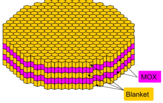
New advanced light water reactors (LWRs) have been proposed with the potential to breed and consume transuranic actinides to achieve a high conversion ratio. To accomplish this, reactors have been designed with different axial layers of fissile and blanket zones. The Hitachi Resource-Renewable Boiling Water Reactor (RBWR) and the Japan Atomic Energy Agency (JAEA) reduced-moderation water reactor (RMWR) are examples of such reactors. The RBWR model AC (RBWR-AC) is a core that operates with mixed oxide fuel (MOX) and has a breeding ratio of 1.01. The core is comprised of two fissile zones sandwiched between axial internal blankets of depleted uranium. Unlike conventional BWRs, these advanced reactor designs are very axially heterogeneous with the fissile zones producing neutrons and the blanket zones consuming them. This paper addresses how this heterogeneity can be modeled using three-dimensional continuous-energy Monte Carlo codes to generate homogenized macroscopic neutron cross sections for full core calculations.
Currently, to simulate full core transients, core simulators such as SIMULATE and PARCS are used.
These codes need burnup dependent few-group homogenized macroscopic cross sections of each type of material in various operating conditions (control rod, fuel temperature, moderator density, etc.). These cross sections are traditionally generated using two-dimensional lattice physics codes such as CASMO or HELIOS on assembly level geometry with either reflective or periodic boundary conditions. Some deterministic codes allow for an axial buckling to try to approximate the shape of the axial flux. Although useful for some applications, this is not feasible for the RBWR since the axial flux shape cannot be characterized with a buckling. The RBWR has significant axial streaming of neutrons from the fissile zones to the blanket zones especially in highly voided regions toward the top of the core. Two-dimensional cross sections may not be sufficient because the RBWR does not have zones with a distinct flux energy spectrum. Rather, the spectrum is continuously changing along the axial direction because of the changing void fraction and material zones, thus making it difficult to decouple zones from each other. Two-dimensional codes are therefore limited in capturing the effects of such heterogeneity.
A comparison can be made between cross sections generated from two-dimensional geometry and those from three-dimensional geometry. The Serpent code is employed in this research. Serpent is a continuous-energy Monte
Carlo lattice physics code1 developed to generate few
group homogenized macroscopic cross sections and other parameters for use in core simulators. Serpent allows for arbitrary geometry and homogenization over any given region of an assembly. This paper describes a procedure for generating few-group, homogenized cross sections from a three-dimensional assembly geometry and compares the results with a traditional two-dimensional assembly homogenization method for a typical high conversion (LWR) such as the RBWR.
II. CROSS SECTION GENERATION METHODS The main core analysis methods in the industry are nodal diffusion theory methods. Full core simulators that use these methods require a database of few-group homogenized cross sections because it takes a prohibitive amount of computing power to solve the core with thousands of energy groups and spatial detail for all depletion and core conditions. Therefore, the generation of few-group, spatially homogenized cross sections is a very important step in the core analysis procedure. The computational scheme for reactor analysis is shown in Fig. 1. The overall calculation scheme for generating cross sections is globally the same, regardless of the approach. It begins with the preparation of neutron reaction cross sections for each nuclide processed into evaluated nuclear data files. The next major step is to perform lattice
calculations, where the few-group homogenized cross sections are generated as a function of various state variables (e.g. burnup, fuel temperature, moderator density etc.), representing all possible operating conditions. The full reactor core simulator then interpolates these cross section datasets produced from the lattice calculation to obtain a local condition-specific set of cross sections for each spatial node. The analyses of transients coupled to thermal-hydraulic feedback and fuel management can then be performed.
Fig. 1. Overall Reactor Analysis Calculation Scheme2 Neutron‐nuclide cross‐section calculation Lattice calculation Depletion calculation Reactor calculation Spatial kinetics calculation Fuel management Design and operation simulation Depletion calculation
The main work in the preparation of few-group cross section datasets lies in the lattice calculation. The traditional approach of generating the cross sections is outlined in Section II.A, where a deterministic approach is utilized. In Section II.B, an alternative approach is described, where Monte Carlo is used in the generation of homogenized cross sections using a three-dimensional assembly calculation.
II.A. Traditional Two-Dimensional Method
The traditional approach of generating cross sections involves the use of deterministic lattice codes. The overall goal in this procedure is to calculate the energy-dependent
scalar neutron flux, φ
( )
r EG, , commonly referred to as fluxspectrum. Once the flux spectrum is known, few-group homogenized cross sections are computed from
(
) (
)
(
)
3 3,
,
.
,
V g g V gd r dE
r E
r E
d r dE
r E
α αφ
φ
Σ
Σ
=
∫ ∫
∫ ∫
G
G
G
(1)In Eq. (1), Σα g represents the spatially-group averaged homogenized macroscopic cross section for group g of
arbitrary type α and Σα
( )
r EG, is the continuousmacroscopic cross section as a function of position and
energy2. This relation represents conservation of reaction
rates, where the flux spectrum is used as the weighting function. If the flux spectrum is known, then the homogenization can take place.
Deterministic lattice codes usually solve the integral form of the neutron transport equation either by a collision probability method or method of characteristics. In each of these approaches, it would be very time consuming to calculate the detailed flux spectrum in thousands of groups. Therefore, approximations to the flux spectrum are made before the lattice calculation. The first step in this procedure is to perform group-wise condensation of cross sections assuming a flux spectrum, which may not represent the actual flux spectrum of the system. This step is carried out in codes such as NJOY in the module GROUPR. Therefore, information about the detailed cross section dependence on energy is partially lost. These calculations are performed for each isotope at different temperatures and dilutions, since the actual configuration of the geometry and operating conditions are not taken into account at this point. The next step typically involves further condensation of groups in a simplified one-dimensional pin cell geometry. One-one-dimensional calculations are performed to get further detail about the flux spectrum including resonance self-shielding effects in different zones of the pin cell. After all of these approximations, a typical neutron library of about 100 groups is produced for the lattice calculation. It is important to note that there are multiple approximations made to the flux spectrum to condense cross sections to a manageable number of energy groups to perform lattice calculations on the assembly level.
At the lattice calculation stage, it is common to only consider dimensional geometry. Each two-dimensional slice of a unique configuration is considered. At this step, there is an implicit assumption that the assembly being considered can be decoupled from the rest of the core. The lattice calculation is then performed at various operating conditions as a function of burnup with reflective or periodic boundary conditions in the radial plane. The final product of this procedure is a macroscopic cross section database that is available for use in full core calculations.
II.B. Proposed Three-Dimensional Approach
The proposed methodology makes use of a three-dimensional Monte Carlo assembly calculation rather than a two-dimensional deterministic approach. Monte Carlo methods are attractive because the actual geometry of the
system can be represented and many of the approximations described in Section II.A do not need to be made. Much work is being done to use both deterministic and Monte Carlo techniques to solve full core geometry. Although not a new idea, there have been several recent studies using Monte Carlo methods to generate few-group homogenized
parameters for full core deterministic calculations3.
A continuous-energy Monte Carlo neutron transport code such as Serpent can be used to generate few-group homogenized cross sections for a full core simulator. Although Monte Carlo codes typically take a long time to run due to the simulation of individual neutrons and the inherent statistical nature of these calculations, they do not make all of the approximations of the traditional approach. Because Monte Carlo is being used at this stage, the point-wise continuous cross section data in the evaluated nuclear data files can be used directly. Compared with the traditional approach, no approximations need to be made for the shape of the flux spectrum to collapse cross sections in a few hundred groups for lattice calculations. In Serpent, the homogenized cross sections are calculated using a collision estimator of the flux where
(
)
(
)
(
)
,
,
.
,
j j j j t j j g j j t j jw
r E
r E
w
r E
α αΣ
Σ
Σ
=
Σ
∑
∑
G
G
G
(2)In Eq. (2), j represents a collision,Σα
( )
rGj,E j is themacroscopic cross section for arbitrary reaction α at
energy
E
j and position rGj at the collision,( )
, jj
r E
t
Σ G is
the total macroscopic total cross section, and is the
statistical weight of the neutron experiencing the collision. In this representation of the homogenized cross section, the flux is the weighting function represented by the number of collisions. This summation is only performed over the region and energy group of interest for the homogenization and therefore takes into account the integral of the reaction rate over space and energy.
j
w
This approach is used in Serpent and has been shown to produce accurate homogenized cross sections for
two-dimensional geometries4. In Serpent, the geometry can be
extended to three-dimensions and homogenized cross sections can be generated for an arbitrary number of homogenization regions. A detailed three-dimensional lattice can be modeled and few-group homogenized cross sections can be extracted for each homogenization region in the core. This will allow for the axial heterogeneity effects present in advanced LWRs to be captured accurately.
III. SCOPE OF WORK
This research is part of a larger effort to develop an accurate procedure for modeling axially heterogeneous LWRs with a high conversion ratio. Modeling the core using two-dimensional cross sections should eventually work as the number of energy groups increases, but this might be avoided by capturing the spectral effects through the generation of cross sections using three-dimensional geometry. This paper investigates and reports the errors that can potentially be introduced when two-dimensional cross sections decoupled from the three-dimensional reactor environment are generated instead of accounting for the three-dimensional heterogeneity. Serpent will be used in both the two-dimensional and three-dimensional assembly calculations so that a consistent comparison is made.
IV. METHOD OF CALCULATION
This section describes the overall method used to compare parameters generated with the influence of neighboring zones from a three-dimensional calculation with traditionally-generated parameters from a two-dimensional calculation.
IV.A. Serpent Cross Section Generation
The Serpent code was developed at VTT Technical Research Centre of Finland. The effort was primarily focused on the use of continuous-energy Monte Carlo for lattice physics applications. Its main feature, used in this analysis, is the ability to generate few-group homogenized parameters for coupled deterministic full core reactor analysis. Because Serpent was intended as a lattice physics code, it includes the generation of homogenized multigroup cross sections, group transfer scattering matrices, diffusion coefficients, assembly pin powers and discontinuity factors, etc. This is extremely useful in that manual tallies do not have to be added to calculate these parameters. This makes the data collection easier for input into a core simulator, which is the eventual goal of this work.
Serpent has the capability of modeling arbitrary geometry and also has built-in types of lattices, which make it convenient to model the RBWR. Significant effort has been put into improving the computational efficiency of Serpent. Two main features of Serpent include the Woodcock delta-tracking method and a unionized energy grid format for its neutron libraries. Serpent has an excellent built-in depletion module so the group constants can be generated as a function of burnup. It reads the continuous-energy cross sections from ACE formatted library files and therefore, the same fundamental interaction data can be used for different geometries and
operating conditions. For all of the calculations present in this paper, the ENDF/B-VII neutron library was used.
IV.B. Assembly Geometry
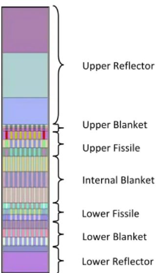
The RBWR is used to investigate the difference between two-dimensionally and three-dimensionally influenced cross sections. A diagram of the RBWR core is shown in Fig. 2. The RBWR core, similar to the RMWR, has five axial fuel zones. The fissile zones, made up of MOX fuel, are sandwiched between internal blanket zones for breeding. The axial zones shown in the full core layout are surrounded at the bottom and top of the core by multiple reflector zones. For the purpose of these analyses, only a single assembly was modeled to isolate the effects of axial and radial heterogeneity. The RBWR assembly has a hexagonal lattice with 271 fuel rods of 5 different
fissile Pu enrichments radially5. In addition, Y-shaped
control rods are inserted between adjacent assemblies.
Fig. 2. RBWR full core layout6.
The RBWR-AC single assembly is modeled in Serpent, and each axial zone is further split into three additional zones to account for the variable moderator void distribution. Top and side views of the modeled geometry are shown in Fig. 3 and Fig. 4, respectively. Each enrichment zone is represented by an unique color in Fig. 3. For this analysis, it is assumed that the Y-shaped control rods are not present and therefore just a bypass flow gap is modeled between assembles. Because hexagonal geometry is used, the model is constrained with periodic boundary conditions. Fig. 4 shows an axial view of the geometry, in which all fuel zones were modeled in detail, while the top and bottom reflector zones are homogenized. This view represents a cut across the center of the assembly shown in Fig. 3. Although the detailed geometry of the reflector could be modeled, it was determined that the effect of modeling the detailed reflectors was small, and thus they are homogenized for simplicity.
IV.C. Generation of Cross Sections
The generation of two-dimensionally and three-dimensionally influenced cross sections can be calculated for each axial zone shown in Fig. 4. The process involves one calculation for the three-dimensional assembly. Here, neutrons are transported around the full detailed geometry and homogenized few-group parameters are generated in each axial zone separately. Therefore, the resulting homogenized cross sections are generated with the influence from axial neighbors.
For the two-dimensional transport calculations, a separate input file was constructed for each axial blanket and fissile zone represented in Fig. 4. These 2-D lattice
calculations are run separately with periodic boundary conditions in all three dimensions with no influence from the neighboring assembly zones. The use of color sets is an option to account for the effects of radial neighbors. The radial effects were not considered here since the primary concern is the treatment of the axial heterogeneity in the RBWR. For each two-dimensional lattice calculation, the few-group parameters are homogenized over the entire geometry.
Fig. 3. Top view of fissile zone of the assembly.
V. RESULTS
This section presents the results from the Serpent calculations. For all calculations, 200 million neutrons were run and parameters were calculated and compared for two groups with the thermal cutoff placed at 0.625 eV. The calculations were performed with 35 Intel Xeon 5620 Quad Core Processors (2.4 GHz) on a Beowulf cluster. The average calculation time for the three-dimensional geometry was 7 hrs, while each two-dimensional calculation took about 2 hrs. The axial zones have been given ID names (from bottom to top) and are listed in Table I.
Fig. 4. Axial view of center of assembly.
Lower Reflector Lower Fissile Internal Blanket Upper Fissile Upper Blanket Upper Reflector Lower Blanket TABLE I Axial Zone ID Names
ID Zone LB1 Lower Blanket Zone 1 LB2 Lower Blanket Zone 2 LB3 LF1 LF2 LF3 IB1 IB2 IB3 UF1 UF2 UF3 UB1 UB2 UB3
Lower Blanket Zone 3 Lower Fissile Zone 1 Lower Fissile Zone 2 Lower Fissile Zone 3 Internal Blanket Zone 1 Internal Blanket Zone 2 Internal Blanket Zone 3 Upper Fissile Zone 1 Upper Fissile Zone 2 Upper Fissile Zone 3 Upper Blanket Zone 1 Upper Blanket Zone 2 Upper Blanket Zone 3
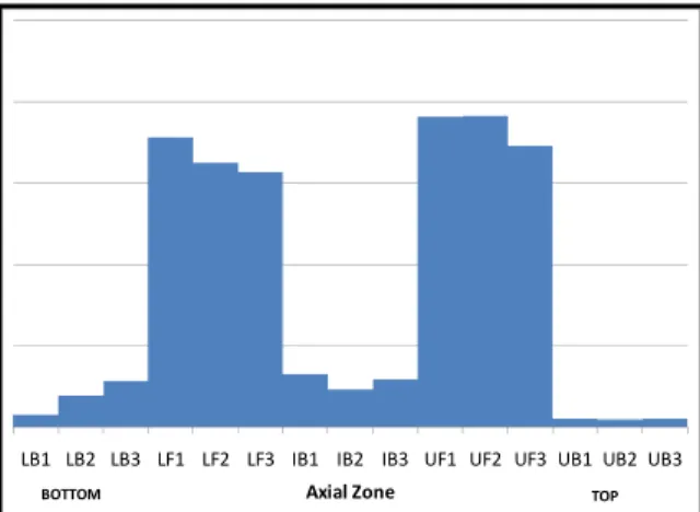
V.A. Axial Power Distribution
To demonstrate the importance of coupling different axial zones, a plot of the axial power distribution at beginning of life is shown in Fig. 5. Fig. 6 presents the power distribution in the fissile regions and the thermal flux in the non-fissile regions. It is clear from these power distribution figures that there is a strong neutron source zone, where neutrons are produced from fission, and zones where neutrons are captured. In Fig. 6, the bright yellow-white color zones along the fuel rods represent the fissile
zones producing most of the power. These zones are surrounded by low power regions shown in dark red. In the non-fueled zones (coolant around fuel rods and reflectors) the white-blue color represents a high thermal flux and the dark blue represents a low thermal flux. At the top of the core, there is a hard spectrum from the
low-voided regions and upper fissile zones. This leads to a high thermal flux peak at the lower part of the upper reflector. In addition, higher thermal fluxes surround the blanket zones because of the absence of plutonium. Modeling the 3-D geometry in the homogenization process to account for
the high degree of axial heterogeneity in these advanced reactors may be essential in full core calculations.
V.B. Flux Energy Spectrum
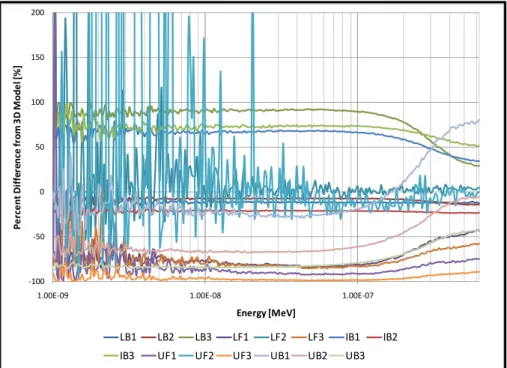
As explained in Section II, the flux energy spectrum is an integral part of the homogenization of group constants. Therefore, errors in the final homogenization are influenced by differences in the energy spectra. For each homogenization region in the 2-D and 3-D geometries, the flux was tallied in 1000 equally spaced lethargy bins, spanning the entire energy range. The energy spectra for the 2-D geometry were then compared to the energy spectra from the corresponding 3-D geometry method. The differences between the 2-D to 3-D geometry in the thermal energy range and the fast energy range are shown in Fig. 7 and Fig. 8, respectively.
Fig. 5. Relative axial power distribution of 3D assembly.
LB1 LB2 LB3 LF1 LF2 LF3 IB1 IB2 IB3 UF1 UF2 UF3 UB1 UB2 UB3
Axial Zone
BOTTOM TOP
Fig. 7 presents differences for each zone in the thermal energy range. At very low energies, the noise in the fissile zone results is mainly due to the statistical uncertainty in the flux. The fissile zones contain MOX fuel and therefore have a harder spectrum. The uncertainty is due to the relative lack of neutrons at these thermal energies. Even though there may be uncertainty on the flux, it is clear that there is a significant difference in many of the zones. Fig. 8 presents the differences in the fast energy range. Here, the Monte Carlo uncertainty in the flux edits is lower because there are many more neutrons at higher energies. It is clear in this plot that there are errors in many of the zones especially at interface regions between the blanket and fissile zones.
(see text for description of colors) Fig. 6. Axial power distribution from Serpent.
Two representative flux energy spectra were chosen to illustrate the differences between a fissile zone and a blanket zone. Fig. 9 shows the energy spectrum of the upper-most zone of the upper blanket (UB3). The two-dimensional calculation predicts a harder spectrum than the three-dimensional calculation. This is expected because the three-dimensional calculation homogenizes cross sections in the presence of the upper reflector, which is a source of thermal neutrons, as shown in the axial power distribution in Fig. 6. Decoupling the upper blanket zone from its axial neighbors (i.e. the upper reflector) may not be appropriate for computing homogenized parameters. In Fig. 10, the flux energy spectrum is shown for the middle region of the lower fissile zone (LF2). Here, the flux spectra from the two- and three-dimensional calculations compare well and there is a smaller difference between them, which is consistent with the results in Fig. 8. There is not much difference in this zone because this zone is surrounded by similar zones. Therefore, the approximation to decouple this zone from neighboring axial zones might be appropriate and there should not be major differences between the homogenized cross sections.
Fig. 7. Thermal energy spectra differences ‐100 ‐50 0 50 100 150 200
1.00E‐09 1.00E‐08 1.00E‐07
Pe rc e n t Di ffe re n ce fr o m 3D Mo d e l [% ] Energy [MeV] LB1 LB2 LB3 LF1 LF2 LF3 IB1 IB2 IB3 UF1 UF2 UF3 UB1 UB2 UB3
V.C. Homogenized Parameters
Since the ultimate goal is to perform full core calculations, the errors seen in the detailed flux spectra will propagate into the few-group homogenized cross sections that are used for the full core nodal calculation. To estimate the magnitude of the error that can propagate to
the full core calculation, two-group macroscopic cross sections are compared. The most important cross sections to examine are the macroscopic absorption cross section,
a
Σ , macroscopic fission production cross section, νΣf ,
macroscopic transport cross section, Σtr, and the group
Fig. 8. Fast energy spectra differences. ‐100 ‐50 0 50 100 150
1.00E‐06 1.00E‐05 1.00E‐04 1.00E‐03 1.00E‐02 1.00E‐01 1.00E+00 1.00E+01
Pe rc e n t Di ffe re n ce fr o m 3D Mo d e l [% ] Energy [MeV] LB1 LB2 LB3 LF1 LF2 LF3 IB1 IB2 IB3 UF1 UF2 UF3 UB1 UB2 UB3
Fig. 9. Flux Energy Spectrum in Upper Blanket Zone 3 0.00E+00 5.00E‐05 1.00E‐04 1.50E‐04 2.00E‐04 2.50E‐04 3.00E‐04 3.50E‐04
1.00E‐10 1.00E‐08 1.00E‐06 1.00E‐04 1.00E‐02 1.00E+00
Fl u x per Le th ar gy [‐ ] Energy [MeV] 3D Geometry 2D Geometry
transfer scattering cross sections represented by
Σ
s g, '→g.Tables II and III present the magnitude of the differences for the neutron fission production cross section and the absorption cross section when produced by 2D and 3D methods.
Because Monte Carlo methods are stochastic, it is also important to look at the uncertainty in the mean values obtained from the calculations. Although not included in
the tables, the statistical uncertainties in all of the values reported were less than 1% relative to the mean value. In each table, results are reported for each axial zone when it is considered in the full three-dimensional assembly and by itself in two-dimensions. The percent differences between the two-dimensional and three-dimensional quantities are also reported, where the 3D calculation is treated as the reference solution. Negative values mean that the
two-Fig. 10. Flux Energy Spectrum in Lower Fissile Zone 2 0.00E+00 1.00E‐04 2.00E‐04 3.00E‐04 4.00E‐04 5.00E‐04 6.00E‐04 7.00E‐04 8.00E‐04
1.00E‐10 1.00E‐08 1.00E‐06 1.00E‐04 1.00E‐02 1.00E+00
Fl u x per Le th ar gy [‐ ] Energy [MeV] 3D Geometry 2D Geometry
dimensional value under-predicts the three-dimensional value.
From Tables II and III, many interesting trends can be observed. First, as expected, there are larger discrepancies between the homogenized cross sections at the top of the assembly. This is mainly due to the harder spectrum of neutrons and the presence of the reflector on the top of the core and the upper fissile zone below the blankets. The spectrum differences for these upper blankets zones are similar to those shown in Fig. 9.
Another interesting result is in the lower fissile zones.
Even though this zone is a strong source of neutrons, there are still significant differences in the thermal homogenized cross sections at the interfaces between the lower blanket zone and the internal blanket zone. In particular, we focus on the neutron fission production and absorption cross sections because they are important to the fission reaction rate. As expected, the middle of the lower fissile zone (LF2) does not show large differences. The neutron spectra comparison shown in Fig. 10 shows a good agreement between these data and therefore, no significant difference is seen after the homogenization process. Thus, TABLE II
Differences in Neutron Fission Production Cross Section
3D Geometry 2D Geometry
Region νΣf1 νΣf2 νΣf1 νΣf2 Diff νΣf1[%] Diff νΣf2 [%]
LB1 0.0030 0.0202 0.0032 0.0202 7.3 0.1 LB2 0.0029 0.0201 0.0032 0.0202 10.6 0.6 LB3 0.0030 0.0195 0.0032 0.0202 5.9 3.6 LF1 0.0302 1.6047 0.0294 1.1169 ‐2.9 ‐30.4 LF2 0.0271 1.1206 0.0273 1.0869 0.8 ‐3.0 LF3 0.0274 1.5400 0.0258 1.0654 ‐5.7 ‐30.8 IB1 0.0023 0.0178 0.0024 0.0183 3.4 2.8 IB2 0.0019 0.0180 0.0023 0.0180 21.2 0.4 IB3 0.0019 0.0171 0.0022 0.0174 11.4 1.7 UF1 0.0185 1.3960 0.0176 0.8937 ‐5.1 ‐36.0 UF2 0.0170 1.8108 0.0166 0.8820 ‐2.0 ‐51.3 UF3 0.0173 1.4744 0.0161 0.8923 ‐6.8 ‐39.5 UB1 0.0023 0.0176 0.0017 0.0153 ‐27.0 ‐12.8 UB2 0.0022 0.0181 0.0017 0.0153 ‐20.9 ‐15.5 UB3 0.0021 0.0186 0.0017 0.0152 ‐20.1 ‐18.0 TABLE III
Differences in Absorption Cross Section
3D Geometry 2D Geometry
Region Σa1 Σa2 Σa1 Σa2 Diff Σa1[%] Diff Σa2 [%]
LB1 0.010 0.030 0.009 0.030 ‐7.3 0.1 LB2 0.010 0.030 0.009 0.030 ‐8.9 0.5 LB3 0.009 0.029 0.009 0.030 4.0 3.2 LF1 0.021 1.041 0.020 0.774 ‐3.7 ‐25.6 LF2 0.017 0.782 0.018 0.758 4.7 ‐3.0 LF3 0.018 1.015 0.017 0.746 ‐6.5 ‐26.5 IB1 0.008 0.025 0.008 0.026 3.3 2.5 IB2 0.009 0.025 0.008 0.026 ‐13.4 0.4 IB3 0.007 0.024 0.007 0.025 5.3 1.5 UF1 0.012 0.923 0.012 0.634 ‐4.3 ‐31.3 UF2 0.011 1.267 0.011 0.627 4.5 ‐50.5 UF3 0.011 0.947 0.011 0.635 ‐4.1 ‐32.9 UB1 0.005 0.024 0.006 0.022 26.8 ‐11.7 UB2 0.006 0.025 0.011 0.627 12.2 14.1
for the lower fissile zone, the middle zone (LF2) can be decoupled from the rest of the assembly without much error. It is evident that for this type of reactor design, it may be important to generate cross sections with the full three-dimensional geometry to capture the axial streaming effects in all core regions.
IV. CONCLUSIONS AND FUTURE WORK A model of the Hitachi RBWR was constructed using the Serpent Monte Carlo code to estimate the error introduced when performing traditional two-dimensional geometry lattice calculations versus three-dimensional geometry in the homogenization process. Two-group homogenized cross sections were generated for each zone with the influence of other zones in the assembly (3-D homogenization) and for the zone by itself (2-D homogenization). Significant differences in flux-energy spectra were observed in zones that were surrounded by different neighboring axial zones and zones located toward the top of the core where there is the presence of an upper reflector and where the coolant void fraction is high. Differences seen in the flux-energy spectra can be observed in the resulting homogenized cross sections. Comparing homogenized cross sections resulted in discrepancies up to 50%. These differences in homogenized cross sections can lead to differences in the full core calculations predicting core power distribution and void coefficient of reactivity. This analysis provides motivation to examine how these differences propagate to the full core analysis.
The results of the research presented here provide motivation to use the Monte Carlo code Serpent to generate homogenized cross section datasets for a full core calculation. An efficient way of calculating these
homogenized cross sections for a range of different operating conditions has not yet been built into Serpent. Currently, Serpent only allows for one state calculation at a time and does not perform branch cases automatically. A preliminary automation tool has been developed to run Serpent for the purpose of generating cross section data sets with branch cases. This tool, developed in Python programming language, allows a user to run Serpent with various operating conditions and organizes the data in a structure that can be used to output cross section data sets in various formats. A cross section data set for use in the
U.S. NRC core simulator, PARCS7 was recently generated
for a two-dimensional PWR assembly as part of this research. Preliminary results are shown in Fig. 11, where k-effective vs. burnup calculations for fuel temperature branches of a typical PWR with Gadolinium pins are plotted. The reference (900 K), high fuel temperature (1500 K) and low fuel temperature (582 K) cases show good agreement between Serpent and PARCS. The differences between them are statistically around zero and are below +/- 40 pcm. This tool will be extended to three dimensional geometries to automatically perform the methodology described in this paper for a range of different operating conditions. Further development of this tool will allow for investigation of these differences to draw conclusions if the traditional methods are sufficient in generating cross sections for this new type of light water reactor.
(a) k-effective vs. burnup comparing Serpent and PARCS (b) difference of k-effective between PARCS and Serpent Fig. 11. Fuel temperature branch (TF) comparison of k-effective between Serpent and PARCS using cross sections generated
from Serpent for a typical PWR with Gadolinium pins.
0.90 0.95 1.00 1.05 1.10 1.15 0.00 5.00 10.00 15.00 20.00 25.00 30.00 35.00 40.00 45.00 k‐ e ffe ct iv e [‐ ] Burnup [MWd/kg]
Serpent TF 582 K PARCS TF 582 K Serpent Ref 900K PARCS Ref 900K Serpent TF 1500 K PARCS TF 1500 K
‐40.00 ‐30.00 ‐20.00 ‐10.00 0.00 10.00 20.00 30.00 40.00 0.00 5.00 10.00 15.00 20.00 25.00 30.00 35.00 40.00 45.00 D if fer en ce [p cm ] Burnup [MWd/kg] TF 582 K TF 900 K TF 1500 K ACKNOWLEDGMENTS
This work was supported by the Rickover Fellowship from the U.S. Department of Energy, Naval Reactors Division. Their support is gratefully acknowledged. This paper was also supported by Professor Mujid S. Kazimi
and the Center for Advanced Nuclear Energy Systems at MIT.
NOMENCLATURE g
α
Σ
homogenized macroscopic group crosssection
(
r E
,
α
Σ
G
)
continuous macroscopic cross sectionas a function of position and energy
(
r E
,
)
φ
G
flux energy spectrum as a function ofposition and energy
j
w
statistical weight of neutron in MonteCarlo
f
ν
Σ
fission neutron production cross sectiona
Σ
macroscopic absorption cross sectionREFERENCES
1. J. Leppӓnen, PSG2/Serpent – a Continuous-energy
Monte Carlo Reactor Physics Burnup Code: User’s Manual, VTT, Espoo (2010).
2. A. Hébert, Applied Reactor Physics. Presses Internationales Polytechnique, Montréal (2009).
3. J. Leppӓnen, Development of a New Monte Carlo
Reactor Physics Code, VTT Publications 640, Espoo
(2007).
4. J. Leppӓnen, “On the Use of the Continuous-energy Monte Carlo Method for Lattice Physics Applications,” Proc. INAC 2009. Rio de Janeiro, Brazil, (2009).
5. Takeda, R. et al, “BWRs for Long-Term Energy Supply and for Fissioning Almost All Transuraniums,”
Proc. of Global 2007, Boise, Idaho (2007).
6. Iwamura, T. et al, “Concept of Innovative Water Reactor for Flexible Fuel Cycle (FLWR),” Nuclear
Engineering and Design, 236, 1599-1605 (2006).
7. Downar, T., Lee, D., Xu Y., Seker, V., 2009. PARCS v3.0: U.S. NRC Core Neutronics Simulator. USER MANUAL, DRAFT (2009).