Application of Hartree-Fock theory of fluctuations to opacity calculation

Application of Hartree-Fock theory of

fluctuations to opacity calculation

By T. BLENSKI AND S. MOREL

IGA, Departement de Physique, Ecole Polytechnique Federate de Lausanne, CH-1015 Lausanne, Switzerland

(Received 23 May 1994; revised 17 January 1995; accepted 19 January 1995)

The Hartree-Fock theory of fluctuations leading to simple formulae for configuration probabilities is used in a Detailed Configuration Accounting calculation of opacity in the case of an iron plasma. A direct Detailed Term Accounting method is also applied. The correlations of subshell occupation numbers, which are accounted for in the HF theory, show small effect on the theoretical spectrum corresponding to conditions of a recent measurement.

I. Introduction

In a previous paper (Blenski & Morel 1993), we described an approach to correlations of the subshell occupation numbers based on the Hartree-Fock (HF) theory of fluctuations. We present here the first results from our opacity program using this approach. Our work is in progress and our first calculations were intended to check the applicability of our method. Our opacity program is based on Detailed Configuration Accounting (DCA) which uses the HF correlation formula to calculate electron configuration probabilities. Our pro-gram also has a Detailed Term Accounting (DTA) option. This option is based on the direct simultaneous diagonalizations of the Hamiltonian and the angular momentum opera-tors. We show as examples some results of our calculations in the case of an iron plasma at 20 eV temperature and at 0.01 density, which is not far from the conditions of a recent experiment (Da Silva et al. 1992). Our goal was to check whether our Detailed Configura-tion Accounting method works correctly. Taking into account the simplicity of the HF theory of fluctuations, this method seems to be a good tool in opacity calculation where a DC A approach is required.

Regarding DCA-DTA option, our objective is to verify whether our DCA method can be applied to opacity calculations when the term structure is taken into account. The DTA calculations reported in the literature (performed with the OPAL code, Iglesias et al. 1987), which demonstrated the importance of the term structure for some low temperature plas-mas, are based on a statistical-mechanics method (activity expansion) which seems to be rather different compared to our approach. Let us stress again that our approach is con-sistent with the average atom approach to the plasma equilibrium and is probably one of the simplest methods which takes into account the detailed configurations. For this rea-son, we were interested in whether the results of our calculations show the redistribution of oscillator strengths predicted by Iglesias et al. (1987) and confirmed experimentally by Da Silva et al. (1992). Another approach using correlations to DCA calculations has also been proposed by Grimaldi and Grimaldi-Lecourt (1982) and Wilson (1993). A method similar to the present one but based on the density functional theory was introduced by Perrot (1988).

In our DTA option, we have used the direct diagonalization method, first proposed by Goldberg et al. (1986), since this method appeared to us to be the simplest one. Now, after the experience of our calculations, we think that this method cannot be directly applied to the full DTA calculations because of its matrix character and necessary restriction in the dimensions of the operator matrices. Perhaps it can still be a candidate for a DTA-UTA approach in which some transition arrays containing few lines are treated using Detailed Term Accounting, while others are accounted for by statistical methods (UTA-Unresolved Transition Array methods; Bauche et al. 1979, 1988).

The paper is organized as follows. We start with a derivation of the thermal average of the absorption cross section using the imaginary part of the dynamic electron polariz-ability (Section 2). Next we neglect the configuration interaction and introduce formally the configuration probability (Section 3). The formula used to calculate this probability is presented in the text, while all details of the HF theory at non-zero temperature and of the HF theory of fluctuations are described in Appendices A and B, respectively. The direct DTA diagonalization is briefly introduced in Section 4, while details of this method may be found in Appendix C. Finally, in Section 5, the numerical results are shown and discussed.

2. Thermal average of the absorption cross section

The thermal averaged atomic absorption cross section can be derived from the formula (Fetter & Walecka 1971; Grimaldi et al. 1985)

'xHtKu), (1)

XR(r,r',t- t') = -l- Tr\P[hHCr,t),nH(f',t'W(t - t'). (2)

n

In equation (2), Tr denotes trace, P is the statistical operator, and nH(r,t) is the electron

density operator in the Heisenberg representation. 6(t — t') is the Heaviside function cor-responding to the causality principle. The statistical operator has the form

P= _{7 y} e

-where H and N are the Hamiltonian and the electron number operator, respectively. Tak-ing the Fourier transform of equation (2) and usTak-ing the Lehmann representation (Fetter & Walecka 1971) leads to

Im

(r,r',w) = -TT(1 - e-"»

) £ P

<n\h(r)\m)(m\n(r')\n)8(hw - (E

where \n) represent Af-electron eigenstates of the Hamiltonian corresponding to the eigen-values En. Eigenvalues of the statistical operator for these states are denoted Pn. The

basis j AI> is complete and contains free electron states. Finally, we obtain for the absorption cross section

with

D

= jdr<n\n{r)-r\m).

In the coordinate representation, h(r) has the form:

n(r) = S 5 ( ^ - 4 ) - (7)

*=i

We see that our initial formula equation (1) already contains the correction for the stim-ulated emission.

The formula, equation (5), is exact. Now we make an approximation and neglect the con-figuration interactions. This allows to write for the bound-bound absorption cross section:

^

K

^

fo> - (E

- £„„,)).

In equation (8), nc and mc run over all initial and final bound electron configurations,

respectively. / and j run over all JV-electron eigenstates of the Hamiltonian in configura-tions nc and mc, respectively. The configuration is characterized by the subshells (in terms

of the principal and the angular quantum numbers) occupation numbers. The configuration probability Pnc is introduced formally in equation (8). At this moment, the only

approxi-mation we have done is to neglect the configuration interactions.

3. Detailed configuration accounting

We assume now that for each configuration, the relative probabilities for all initial eigenstates belonging to nc are nearly equal; that is, we assume that in equation (8),

Pnc,i/Pn<. = 1/Nsc where N!-c is the number of these initial states, that is, the number of all

its Slater determinants. We take into account, however, the exact positions of the lines (within the approximation neglecting the configuration interactions) and exact values of the oscillator strengths by diagonalization of the N-electron Hamiltonian for each initial and final configuration. We assume also that PKc can be calculated using the probability

of the spherically symmetric fluctuations in the HF theory (Appendix B).

The configurations are introduced as follows. First, the fractional occupation numbers of the subshells in the self-consistent HFS atom will be cut to the nearest integers (Gold-berg et al. 1986). We obtain in this way an electronic configuration which is called the most probable configuration. In the next step, we create different atomic configurations by mov-ing electrons from one subshell to another (includmov-ing ionization) and takmov-ing into account the Pauli principle. We create in this way all possible configurations of bound electrons, in ground and excited states. Each configuration n0 is characterized by the set of (integer)

deviations of the occupation numbers 8q°, with respect to the occupation numbers of the most probable configuration qnl. We take as the probability of the n0 configuration:

PB0[fi<,,,/ 6 5 ] = C<fl>exp - ^ K i A ^ X J (9)

using the variances obtained in the HF theory of spherically symmetric fluctuations (Appen-dix B). C(B) is the normalization constant.

4. Detailed term accounting

In the diagonalization of the Hamiltonian and the angular momentum operators, two coupling schemes are applied: the intermediate and the LS (Russell-Saunders) couplings (Cowan 1981).

In the first case, we look for the common eigenstates \nc,i) of the operators [J2,H],

where H is the Hamiltonian and J is the total angular momentum operator. As noted in Goldberg et al. (1986), the diagonalization may be performed in the subspace of eigenstates corresponding to the smallest non-negative value M"cmin of the operator Jz.

In the second case, we simultaneously diagonalize the operators [L2,S2,H] with L and § being the orbital angular momentum and spin operators, respectively. Similarly, as in the case of the intermediate coupling, only the states corresponding to the subspace of the smallest non-negative eigenvalues M£c = 0 and M!}c = 0, \ of the operators Lz and Sz,

respectively, are to be considered. For details, see Appendix C.

5. Numerical results and conclusions

5.1. Correlations of subshell occupation numbers

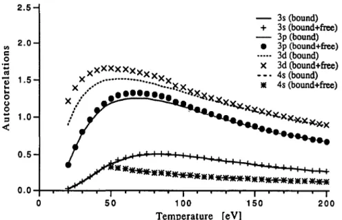
The importance of interaction in the auto-correlations (i.e., in the diagonal terms, GIT1; see equation (B14)) of subshell occupation numbers in the case of solid density iron has been presented in Blenski and Morel (1993). Let us recall that only in the case of the 3d subshell are the interactions with other subshells important, especially at low temperatures. The interactions of bound electrons with free electrons were less important than the inter-actions between bound electrons. We present numerical results which confirm this obser-vation in figure 1. Let us remark here that it would be interesting to check the continuity

2.5H 0.0 3s (bound) + 3s (bound+free) 3p (bound) • 3p (bound+free) 3d (bound) X 3d (bound+free) - 4s (bound) * 4s (bound+free) ************** •x-x 50 _{100 150} Temperature [eV]

FIGURE 1. Autocorrelation versus temperature of the subshell occupation numbers for iron plasma of solid density. Effect of free electrons. The continuous lines correspond to the autocorrelations calculated with the interactions between bound electrons taken into account and with the neglected interactions between bound and free electrons. The points correspond to calculations with the inclusion of interactions between bound and free electrons.

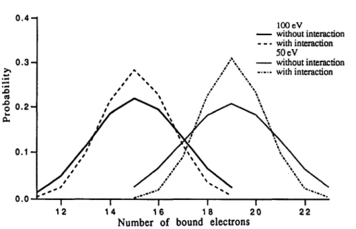
of correlations in the case of pressure ionization (More 1985). Indeed, if the correlations between a bound level, which is close to be pressure-ionized, and the rest of the bound lev-els are important, then after the pressure ionization, when the mentioned level appears as a resonance in the free spectrum, we should find that the correlations between the free and bound spectrum are important. In the present calculations, however, the free levels were treated within the approximation such that only these parts of their wave functions, which are inside the Wigner-Seitz sphere, are taken into account. This problem needs a solution in the frame of a common formalism for bound and free electrons (Blenski & Cichocki 1992). Figure 2 presents the ion charge distributions for solid density iron around the charge of the most probable atom for two temperature values, 50 and 100 eV. The distribution on the right corresponding to 50 eV shows a larger effect of the inclusion of interactions. At 50 eV, the 3d subshell occupation auto-correlation exhibits large dependence on inter-actions (Blenski & Morel 1993).

5.2. Examples of DCA and DTA calculations in the case of iron plasma

In the opacity program, we take into account only orbitals with a principal quantum num-ber up to n = 5 and neglect states with higher n. We use average atom (AA) photoionization (bound-free) cross sections so the edge splitting is not included. AA inverse bremsstrah-lung (free-free) cross sections are also taken. The line shapes are in the form of Voigt func-tions. The physical broadening mechanism includes electron impact, Stark and Doppler broadenings (Rozsnyai 1977). The results we present here are preliminary. We focus our attention on frequency-dependent spectra.

All calculations concern the case of iron at 20 eV temperature and at 0.01 g/cm3 den-sity. These parameters are not very far from the conditions of the Da Silva et al. (1992) experiment. 0.4-1 0 . 3 -IS 0 . 1 -0.0-1 1 100 eV without interaction — with interaction 50 eV /\_ without interaction •' \ with interaction 12 14 16 18 20 Number of bound electrons

i

22

FIGURE 2. Distribution in the number of bound electrons with our probability model in the case of iron at solid density. The results for two temperature values are presented: 50 eV (right) and 100 eV (left). In both cases, the distributions obtained with and without interactions are presented.

10 - |

60

10

2 0 40 6 0 8 0 Photon energy [eV]

100 120

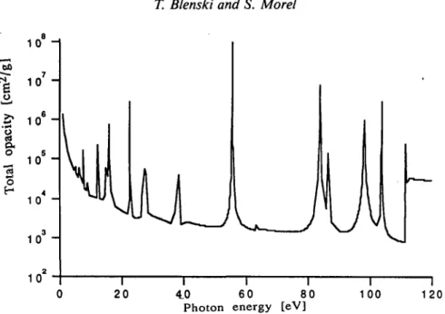
FIGURE 3. Total opacity for iron plasma at 20 eV temperature and at 0.01 g/cm3 density. Indepen-dent electron model (average atom). Number of transitions bound-bound: 40.

Figure 3 displays photoabsorption versus photon energy obtained using the independent electron cross-section formula with the average atom wave functions and energies (i.e., only one average atom configuration with the fractional occupation numbers is used). There are 40 transitions and the strongest line comes from the nonhydrogenous 3p -> 3d transition. This line corresponds to 57 eV photon energy.

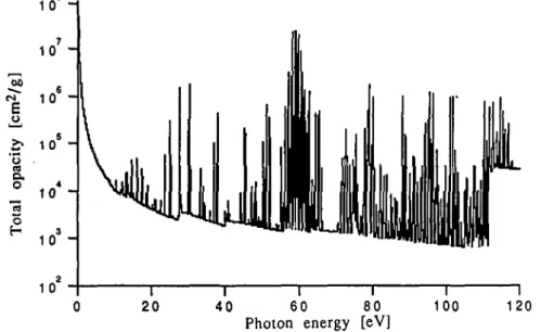
Figures 4 and 5 present results of the DCA calculations in which the term structure is neglected. The energy of each DCA line is taken as the difference between the total con-figuration average energies of the initial and final states. We notice that the DCA approx-imation redistributes the 3p ->3d transitions symmetrically around the 60 eV photon energy. Both curves are similar, which means that the increase of the number of configurations has little impact on the final result.

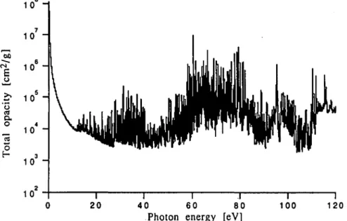
Figures 6 and 7 present results of calculations in which some transition arrays (by tran-sition array we mean all lines between two definite configurations) have been treated using the DTA approach. The criterion for the DTA treatment was that the dimensions of the diagonalized matrices be smaller than 200. We observed that both in the LS and in the inter-mediate coupling, only a part of the DCA lines was subject to the term splitting. This part was larger in the case of the LS splitting (about half of the DCA lines) since the criterion M"LC = 0 and M£c = 0, | , in the LS case reduces more effectively the number of states than

the criterion M"cm/n = 0, 3, in the intermediate case. Nevertheless, the number of lines

even in the LS case was insufficient to fulfill the UTA structure present in figure 7 between 55 and 90 eV. The total Rosseland opacity increases from 4618 cm2/g in the DCA calcu-lation (figure 5) to the value 11302 crnVg in the case of the DTA-LS calcucalcu-lation (figure 7). We notice that the last value is smaller by at least a factor of 2 than the value obtained in DCA-UTA calculations (Blenski & Morel 1995). On the other hand, from the qualitative point of view, the spectra from both figures 6 and 7 confirm the observation made by Da Silva et al. (1992). We see the redistribution of the DCA lines situated around the 60 eV to the large UTA structure appearing in the DTA calculations between 55 and 90 eV.

10"

1 0 _T

40 60 80 Photon energy [eV]

FIGURE 4. Total opacity for iron plasma at 20 eV temperature and at 0.01 g/cm3 density. DCA model. Number of transitions bound-bound: 670. Number of initial configurations taken into account in the calculation: 29. Number of possible electron configurations: 37785.

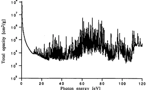
Finally, an interesting question appears: What is the role of the interaction term in equa-tion (B10) on the probability of configuraequa-tions and on the calculated opacity spectrum? Figure 8 displays the result of the calculation in which the uncorrelated probabilities have been used (i.e., equation (B19)). Comparing figure 8 with figure 7, we see that in the

ana-10 10 ₁ 2 0 40I 60I Photon energy | 80 [eV] 100 120

FIGURE 5. Total opacity for iron plasma at 20 eV temperature and at 0.01 g/cm3 density. DCA model. Number of transitions bound-bound: 362517. Number of initial configurations taken into account in the calculation: 13079. Number of possible electron configurations: 37785.

10

10 _T

20 40 60 80 Photon energy [eV]

100 120

FIGURE 6. Total opacity for iron plasma at 20 eV temperature and at 0.01 g/cm3 density. DTA model, intermediate coupling. Number of transitions bound-bound: 180310. Number of initial con-figurations taken into account in the calculation: 29. Number of possible electron concon-figurations: 37785.

lyzed case, the role of interactions seems to be small since both spectra are very similar. The difference in the calculated Rosseland opacities in two cases was inferior to 6%. The reason for this behavior may be the fact that the subshell 3d, which is subject to large cor-relations with other subshells (Blenski & Morel 1993) at small temperatures, appears only as final state in important lines.

10 1 4 0 Photon 1 60 energy i 80 [eV] i 100 I 120 20

FIGURE 7. Total opacity for iron plasma at 20 eV temperature and at 0.01 g/cm3 density. DTA model, LS coupling. Number of transitions bound-bound: 100741. Number of initial configurations taken into account in the calculation: 29. Number of possible electron configurations: 37785.

1 08

1 0 _I

20 40 60 80

Photon energy [eV]

100 120

FIGURE 8. Total opacity for iron plasma at 20 eV temperature and at 0.01 g/cm3 density. DTA model, intermediate coupling. The probabilities of configurations are calculated without interactions. Number of transitions bound-bound: 180310. Number of initial configurations taken into account in the calculation: 29. Number of possible electron configurations: 37785.

In conclusion, we state that the HF theory of fluctuation may be applied to DCA and DCA-DTA calculations of opacity spectra. We obtain qualitatively the main features observed in the experiment (Da Silva et al. 1992). The limitations of the DTA direct diag-onalization method, which we have used, are responsible for too small number of lines in our calculations, which leads to the underestimation of the Rosseland mean opacity. The direct diagonalization method may be useful for small-Z atom calculation or as a supple-ment to a statistical UTA-type approach.

Acknowledgment

The authors would like to thank Drs. B. Cichocki and F. Grimaldi for discussions and critical comments. This research has been partially supported by the Swiss Federal Office for Science and Education (European Network "High Energy Density Matter"), "Union des Centrales Suisses d'Electricite" and Swiss National Science Fund.

REFERENCES BAUCHE, J. et al. 1979 Phys. Rev. A 20, 3183.

BAUCHE, J. et al. 1988 Adv. Atom. Molec. Phys. 23, 131.

BLENSKI, T. & CICHOCKI, B. 1990 Phys. Rev. A 41, 6973.

BLENSKI, T. & CICHOCKI, B. 1992 Laser Part. Beams, 10, 303.

BLENSKI, T. & MOREL, S. 1993 Nuovo Cimento A 106, 1781.

BLENSKI, T. & MOREL, S. 1995 in preparation.

COWAN, R.D. 1981 The Theory of Atomic Structure and Spectra (University of California Press, Berkeley).

CROWLEY, B.J.B. 1990 Phys. Rev. A 41, 2179.

FELDERHOF, B.U. 1969 7. Math. Phys. 10, 1021.

FETTER, A.L. & WALECKA, J.D. 1971 Quantum Theory ofMany-Particle Systems (McGraw-Hill, New York).

GOLDBERG, A. et al. 1986 Phys. Rev. A 34, 421.

GRIMALDI, F. & GRIMALDI-LECOURT, A. 1982 J. Quant. Spectros. Radiat. Transfer 27, 373. (See also F. Grimaldi, In Proceedings of Conferences on Radiative Properties of Hot Dense Matter, Sar-asota (1985, 1992).

GRIMALDI, F. et al. 1985 Phys. Rev. A 32, 1063.

IGLESIAS, C.A. et al. 1987 Ap. J., 322, L 4 5 /

LANDAU, L. & LIFCHITZ, E. 1967 Physique Statistique (Editions Mir, Moscou).

MAHAN, G.D. & SUBBASWAMY, K.R. 1990 Local Density Theory of Polarizability (Plenum, New York).

MERMIN, N.D. 1963 Ann Phys. (N. Y.) 21, 99. MORE, R.M. 1985 Adv. At. Mol. Phys. 21, 305. ROZSNYAI, B.F. 1972 Phys. Rev. A 5, 1137.

ROZSNYAI, B.F. 1977 /. Quant. Spectros. Radiat. Transfer 17, 77.

PERROT, F. 1988 Physica A 150, 357.

WILSON, B.G. 1993 J. Quant. Spectrosc. Radiat. Transfer 49, 241. APPENDIX A: Average atom

We start with an average atom (Rozsnyai 1972; Blenski & Cichocki 1990) submerged in a partially ionized plasma. The electron density of bound and free electrons is obtained via the Schrodinger states. The atomic potential is nonzero only inside the Wigner-Seitz sphere, which is neutral. The average atom results from thermal average over all electronic and ionic states of the plasma when overlapping of the ionic spheres is neglected (Crowley 1990). Another method leading to the average atom is the cluster expansion in the ionic configu-rations (Blenski & Cichocki 1992). The description of the thermal Hartree-Fock theory of electrons may be found in Mermin (1963), Felderhof (1969), and Thouless (1960,1961). The Hartree-Fock equations, which result from minimization of the grand thermodynamic potential fi(p) with respect to the electron density matrix p, are:

s, = e,, = tu + Va + £ < in | v | in )~Pn, (A2)

where p, is the electron density matrix, tu is the kinetic energy, Vu the potential energy:

Vtt = (i

-Ze2

(A3) \r\

and the electron-electron interaction has the form:

{in\v\jm) = {in\vee\jm) - (in\vee\mj), (A4)

where

^ = T T A T 7 - (A5) In equations (A1-A2), the values of energy e, are measured with respect to the chemical potential. The wave-function basis used in the above formulas is that which diagonalizes the matrices p and 7 (Mermin 1963). The one-electron states | /> describe here all solutions

to the Hartree-Fock self-consistent equations A1-A5. These states may be bound or free. In the fluctuation theory (Appendix B), the free electron wave function will be taken as different from the plane wave only inside the Wigner-Seitz sphere. The Hartree-Fock-Slater equations for the average atom are the same as equations (A1-A5), except that in equa-tion (A4), the exchange term is replaced by an exchange-correlaequa-tion potential. The model takes into account mean-field interactions of the bound and free electrons inside this sphere.

APPENDIX B: Fluctuations near the average atom equilibrium

The corrections to the density matrix, bpy, result in the following second order devia-tion of the grand thermodynamic potential, 82U, from its equilibrium value (Mermin 1963; Felderhof 1969):

j > (Bl)

where

(ij\U\mn) = (^^-)8im5jn + <in\v\jm>, (B2)

V Pi - PJ /

and where the summation runs over all electronic states, bound and free.

Equation (Bl) shows that the fluctuations around the Hartree-Fock equilibrium are characterized by pairs of states rather than by occupations of levels. The matrix 8p is nondiagonal since 8p in general does not commute with the matrix p. We will, however, consider, in what follows, only 8p that are diagonal. They correspond to 8p which can be described in terms of fluctuations of the occupation numbers. One then has:

<H\U\m = T-r. r r 5// + Oj\v\ij>, (B3) \P,(1 - Pi)) and 1 where «P/ • 5/5,/. (B5) In the summation in equation (B3), the index belongs to bound {B) or free (F) spec-trum. Further approximation is the assumed spherical symmetry of fluctuations. Using the spherical electronic waves functions leads to:

and this approximation means that the corrections to the occupation numbers will depend only upon the principal /?, and angular /,, quantum numbers:

Spni.li.mi.Si - f>Pn,,l,> (B7) that is, that the distribution among different magnetic and spin quantum numbers is uniform:

= 2 &P»l.l,6pnj.lJ S «V>«|V> " W\Vee\Ji»- (B8)

nhl, m,,Si

These approximations lead to:

V = ^ S «P/<«IU\jj)b~pj = S 8p»,./,fiP-_{7 y} 7.(,^'. (B9>

<-,> n,,i,

nj.lj

with (Blenski & Morel 1993)

0 + 1) \ W / , ( 1 -Pn,.l,)/

I, k lj

We introduced the notation

5p, = 6pni>// = 2(2/, + l)5pn,,,,. (Bll)

The Slater radial integrals and Wigner 3/ coefficients are defined in the usual way (Cowan 1981):

Since we are interested in fluctuations of bound levels occupations, the above formula should be averaged over all possible fluctuations of free levels:

P[bphi G B] = f" . . . f °° n dbpkP[bPi,i G B,F]. (B12)

J-a, J-a, *ef

Taking [bpi,i G F] as varying from minus to plus infinity violates the Pauli exclusion principle. Let us note, however, that for higher values of bph the probability will be very

small and the changes introduced by this approximation may be negligible (Landau & Lifchitz 1967).

In practical calculations, the continuous free spectrum will be discretized. Let us intro-duce the following simplifying notation: The vector bp/ i G B,F will be denoted as bp. Its part corresponding to bound states, bph i e B, will have the index (1), 5p(1), and its free

part, bpi\ i G F, the index (2), bp{2). This convention will also be applied to other vectors

and to the matrix X and its inverse.

The integrations of equation (B12) can be performed analytically and we obtain:

P[bPhi G B] = c^e-G(S"^)/2, (B13)

G(bp0)) = 5p( 1 )^f( U )5p( 1 ) - 6p(i)A'(li2)[A'(2,2)]~1Ar(2>i)6p(1). (B14)

Equation (B14) gives the probability for a set of bph i G B, which represent corrections to

average atom occupation numbers. Both excited states and states of different ion charge may be taken into account.

We may also consider fluctuations that preserve neutrality of the atom. Indeed, one may write:

P[b

i G B,F] = C<*

> e x p f - i 5

« W £ bp), (B15)

where b denotes the Dirac delta.

The neutrality condition, standing in equation (B15), will be written using the vector D (defined as: D, = 1, for / G B,F), and again with our convention, £>(1) and £>(2). We

then have:

Performing the integration over free electron occupation numbers, we obtain:

P[bPi,i GB]= C(B) e x p ( - i G ( 5 p( 1 )) ) , (B17) where G now has a third additional term:

(B18)

Let us remark finally that if the interactions are totally neglected, we have the simple expression:

pip. / _(B19)

APPENDIX C: Direct detailed term accounting

Cl. Intermediate coupling

In this case, the Af-electron states are completely determined by the quantum numbers (Enc, Jnc, M"c), where Enc denote eigenvalues of the operator H, Jnc eigenvalues of the

oper-ator J2, and M"c eigenvalues of the operator Jz of the states belonging to the

configura-tion nc. The summation over i and,/ in equation (8) is replaced by the summation over the

quantum numbers [Enc,Jnc,M"c} and {Enc, Jnc,M™c). Only the diagonalization of the

oper-ators J2 and H in the subspace associated to the smallest value M"cmin should be considered. For that reason, only the matrix elements of the type (Enc, Jnc,M£min | S rk \ Emc, Jmc, M ^i n) can be calculated. We shall express therefore the sum over M"c and Mfc by these matrix elements.

The Wigner-Eckart theorem (Cowan 1981, p. 307) allows us to express the matrix ele-ments of the dipole operator 2 rk by the matrix elements of the reduced dipole tensor P( 1 >:

£ 1 nc> J_n c> N k=l F (Cl) w h e r e i s t h e w i8n e r V coefficient (Cowan 1981, p. 142).

This Wigner 3y coefficient standing in equation (C.I) is different from zero only if

-M"c + q + M™c = 0. However, Mj^min = Af™^in, and the sum over q contains only

q = 0 element. We therefore have

E I M1c • N k=\ 1 J, 0 F I t -'mc > J mc >' ', mm \{Enc>Jnc\\Y^\\Emc,Jmc)\2. (C2)

The sum over M"c and M™c in the matrix elements of the dipole operator becomes: N k=\ m <= J \2 •>rr, ^nc > •'«£. > ^ * y,Cmin I —M"cmin 0

We now use the sum rule for the Wigner 3y coefficients (Cowan 1981, p. 145):

h

• (C3)

where b(jJ2Ji) equals 1 or 0 if j l,j2, andy3 satisfy or do not satisfy the triangle

inequal-ities, respectively. We finally obtain

Af " N F J Mm<: mc> t 'm 0 _{y, mm} (C6)

and obtain for the bb absorption cross section the following results:

^ S S S

Within the approximation that the configuration interactions are neglected, the N-electron states \Enc,Jnc,M£min) and \Emc,Jmc,MT,cmm) c a n be expressed in the basis of Slater

deter-minants belonging to the initial and final configuration, respectively:

\Emc,Jmc,M^min) = J ] (%c}U\Emc,Jmc,M7,cm>n>\*mc,u> = 2 M«| V . « > - (C g)

u=\ u=[

We recall that Nsc and Nsc denote the number of Slater determinants of the configura-tions nc and mc, respectively.

Pn i C _m c Enc,Jn<: Emc,Jm

E

/=!

E>;

'

1 \

where {<?""•',... ,<p%'') and {ip™^",... ,^A/C 1_{"} are the sets of one electronwave functions}

of the Slater determinants $n c i, and ^m<.iU, respectively. Using the properties of the matrix elements involving the Slater determinants (Cowan 1981), we finally obtain:

p

—

— v y v

xb(ho>-(E

-E

))

s s

1

The matrix elements {if>"rc-'\f\^ctU), containing one electron wave functions which are

different in both configurations, are calculated using the formulae from Bethe and Salpeter (Cowan 1981, p. 253).

C2. LS coupling (Russell-Saunders)

In this case, the TV-electron states are determined by the quantum numbers [Enc,Lnc,

Snc,M1f,Msc} where En<: denote eigenvalues of the operator H,Lnc eigenvalues of the

oper-ator L2,Snc eigenvalues of the operator S2, M£c eigenvalues of the operator Lz, and M£c

eigenvalues of the operator Sz.

The summation over / and j in equation (8) is replaced by the sum over the quantum numbers EKc, Lne,Snc,Mp, M§c, Emc, Lmc, Smc, M^, and M?*. Only the diagonalization

of the operators L2, S2, and H in the subspace corresponding to the smallest values of M[f = 0 and M§c = 0, {, is to be performed.

The sum over M£c can be treated in the same manner as the sum over M"c in Sec-tion C l . The sums over M$c and over Nf™c result in the factor 2S + 1. Using the same notation as in the preceding section, we obtain for the absorption cross section in the LS coupling: 3c

- «-*""•> s S s s s

8(L

L

l)5(hw-(E

-E

))

. (CIO)

Since in this case we have only one possibility, Af£min = 0, we may directly use (Cowan 1981, p. 145)

Lm V _ max(Lnc,Lmc)

0 0 0 / (2L

+l)(2L

+l)