Applications of the Bayesian Approach
for Experimentation and Estimation
by
Patrick A. P. de Man
M.Sc. Chemical Engineering
Eindhoven University of Technology, 1998
M.S. Chemical Engineering Practice
Massachusetts Institute of Technology, 2003
SUBMITTED TO THE DEPARTMENT OF CHEMICAL ENGINEERING
IN PARTIAL FULFILLMENT OF THE REQUIREMENTS FOR THE DEGREE OF
DOCTOR OF PHILOSOPHY IN CHEMICAL ENGINEERING PRACTICE
AT THE
MASSACHUSETTS INSTITUTE OF TECHNOLOGY
MASC(HUS~rrS IN$SrrUT~ OF TECHNOLOGY JUNE 2006
© 2006 Massachusetts Institute of Technology
All rights reserved
LIBRARIES
LIBRARIES
AR~CHAIES
Signature of Author...
Department of Chemical Engineering
May 18, 2006Certified
b
y
... . ...
Cetiie"."
Gregory
J.
McRae
Hoyt C. Hottel Professor of Chemical Engineering
Thesis Supervisor
Applications of the Bayesian Approach
for Experimentation and Estimation
by
Patrick A. P. de Man
Submitted to the Department of Chemical Engineering on May 18, 2005 in Partial Fulfillment of the Requirements for the Degree of Doctor of Philosophy in
Chemical Engineering Practice
Abstract
A Bayesian framework for systematic data collection and parameter estimation is proposed to aid experimentalists in effectively generating and interpreting data. The four stages of the Bayesian framework are: system description, system analysis, experimentation, and estimation. System description consists of specifying the system under investigation and collecting available information for the parameter estimation. Subsequently, system analysis entails a more in-depth system study by implementing various mathematical tools such as an observability and sensitivity analysis. The third stage in the framework is experimentation, consisting of experimental design, system calibration, and performing actual experiments. Finally, the last stage is estimation, where all relevant information and collected data is used for estimating the desired quantities.
The Bayesian approach embedded within this framework provides a versatile, robust, and unified methodology allowing for consistent incorporation and propagation of uncertainty. To demonstrate the benefits, the Bayesian framework was applied to two different case studies of complex reaction engineering problems. The first case study involved the estimation of a kinetic rate parameter in a system of coupled chemical reactions involving the relaxation of the reactive O('D) oxygen atom. The second case study was aimed at estimating multiple kinetic rate parameters concurrently to gain an understanding regarding the reaction mechanism of the oxygen addition to the transient cyclohexadienyl radical.
An important advantage of the proposed Bayesian framework demonstrated with these case studies is the possibility of 'real-time' updating of the state of knowledge regarding the parameter estimate allowing for exploitation of the close relationship between experimentation and estimation. This led to identifying systematic errors among experiments and devising a stopping rule for experimentation based on incremental information gain per experiment. Additional advantages were the improved
understanding of the underlying reaction mechanism, identification of experimental outliers, and more precisely estimated parameters.
A unique feature of this work is the use of Markov Chain Monte Carlo simulations to overcome the computational problems affecting previous applications of the Bayesian approach to complex engineering problems. Traditional restricting assumptions can therefore be relaxed so that the case studies could involve non-Gaussian distributions, applied to multi-dimensional, nonlinear systems.
Thesis Supervisor: Gregory J. McRae
Acknowledgments
In these matters the only certainty is that nothing is certain.
Pliny the Elder
My five years at MIT have made an enormous impact on my life. I feel very fortunate to have had the opportunity to spend time in this exciting institute. Certainly, I never even imagined of my career change from engineering to finance. This journey could not have been possible without the support of a number of people to whom I would like to express my gratitude.
The person whom I am forever grateful is my wife Mika, who sacrificed a lot in order to be with me here at MIT. She has provided unwavering support during the many
strenuous moments.
I extremely enjoyed working with and learning from my advisor Gregory McRae. He provided insightful guidance on both professional and personal level and gave me the push in the back I needed every now and then.
The two case studies in this thesis were based on the research of Dr. Edward Dunlea and of Dr. James Taylor. Ed and James have been very generous with their time in explaining their work and answering my endless questions.
During my research the thesis committee members always gave me thoughtful and helpful comments and questions. I would like to thank Prof. Kenneth Beers, Prof. Charles Cooney, Prof. William Green, Prof. Klavs Jensen, Prof. Dennis McLaughlin, Prof. Mario Molina, and Dr. Mark Zahniser.
Special thanks go to Sara Passone for our joint effort of learning the Bayesian approach and for proofreading my thesis, and to Ico San Martini and Jose Ortega for their advice on the Bayesian approach and Markov Chain Monte Carlo. Last but not least, thanks to my other colleagues Barthwaj Anantharaman, Nina Chen, Jeremy Johnson, Chuang-Chung Lee, Mihai Anton, Alex Lewis, Anusha Kothandaraman, and Bo Gong of the McRae research group for providing the sunshine in our windowless basement office.
Table of Contents
1. Introduction...17
1.1 Thesis Statem ent ... 17
1.2 M otivation ... 18
1.2.1 Complex Problem s ... 19
1.2.2 Description of the Bayesian Approach ... 21
1.2.3 The Relevance of Non-Gaussian Distributions ... 23
1.2.4 Acceptance of the Bayesian Approach ... 24
1.3 Objectives ... 25
1.4 Thesis Outline ... 26
2. Characterization of Uncertainty
...
29
2.1 Introduction ... 29
2.1.1 Accuracy and Precision ... 29
2.1.2 Uncertainty, Error, and True Value ... 30
2.2 M easurem ent Error ... 32
2.2.1 Central Lim it Theorem ... 32
2.2.2 Random Error: Instrument Noise and Process Variability ... 33
2.2.3 Error M odel ... 34
2.2.4 Influencing Measurement Error ... 35
2.2.5 System atic Error ... 36
2.3 Limitations of Conventional Statistics ... 37
2.3.1 Linear Error Statistics ... 37
2.3.2 Nonlinear Approxim ations ... 38
2.3.3 Error Propagation ... 40
2.3.4 Abuse of the Central Limit Theorem ... 42
3. The Bayesian Approach
...
45
3.1 Introduction ... 45
3.1.1 Inescapable Uncertainty ... 45
3.1.2 Reasoning ... 46
3.1.3 Inductive Logic ... 47
3.1.4 Degree of Belief ... 47
3.1.5 Illusory Random ness ... 48
3.2 Probability Theory ... 49
3.2.1 Conventional Definitions ... 49
3.2.3 The False-Positive Puzzle ... 53
3.3 The Bayesian Approach ... 56
3.3.1 Bayes' Theorem ... 56
3.3.2 A 'Learning' Algorithm ... 57
3.3.3 Prior Distribution ... 59
3.3.4 Likelihood Function ... 60
3.3.5 Exploitation of the Posterior Distribution ... 61
3.4 Bayes' Theorem and Common Estimation Methods ... 63
4. Bayesian Computation: Markov Chain Monte Carlo
...
65
4.1 Introduction ... 65
4.2 Markov Chain Monte Carlo ... 66
4.2.1 Rationale ... 66
4.2.2 Properties ... 66
4.2.3 Summ arizing Variables ... 68
4.3 Metropolis-Hastings Algorithm ... 69 4.3.1 Background ... 69 4.3.2 Probing Distribution ... 70 4.3.3 Acceptance Probability ... 71 4.3.4 Algorithm ... 72 4.3.5 Algorithm Illustration ... 72
4.4 Num erical Error ... 74
4.4.1 Random Number Generator ... 74
4.4.2 Number of Samples ... 75
4.4.3 Number of Bins ... 76
5. Parameter Estimation
...
77
5.1 Literature on Bayesian Parameter Estimation ... 77
5.1.1 Hierarchical M odels ... 78
5.1.2 Linear Regression with a Change Point ... 78
5.1.3 Non-Conventional Parameters ... 79
5.1.4 Num erical Robustness ... 79
5.2 Formulation for Bayesian Parameter Estimation ... 80
5.2.1 Likelihood Function ... 80
5.2.2 Prior Distribution ... 82
5.3 Advantages of Bayesian Parameter Estimation ... 84
5.4 Param eter Estim ation Strategies ... 86
5.4.1 Sequential Estim ation ... 86
5.4.2 Parallel Estim ation ... 87
5.4.3 Simultaneous Estim ation ... 90
5.5.2 The Bayesian Approach ... 92
5.5.3 MCMC Implementation ... 92
5.5.4 Initial Design ... 93
5.5.5 Covariance Matrix of the Probing Distribution ... 93
5.5.6 Burn-in Period and Convergence ... 95
5.5.7 Thinning ... 98
5.5.8 Estimation Results ... 99
5.5.9 Comparison to Linear Regression ... 99
6. Framework for Experimentation and Estimation
...
101
6.1 Introduction ... 101
6.2 System Description ... 103
6.2.1 Reaction Mechanism and Mathematical Model ... 103
6.2.2 Physical Constraints and Relationships ... 103
6.2.3 Proposed Experiment ... 104 6.3 System Analysis ... 104 6.3.1 Degrees of Freedom ... 104 6.3.2 Observability ... 106 6.3.3 Concentration Profiles ... 107 6.3.4 Rate of Reactions ... 108 6.3.5 Sensitivity Analysis ... 108
6.4 Experimentation and Estimation ... 109
6.4.1 Model-Based Experimental Design ... 109
6.4.2 System Calibration ... 110
6.4.3 Recording Information ... 110
6.4.4 Objective Function ... 110
6.4.5 Bayesian Parameter Estimation Framework ... 111
6.4.6 Data Discrimination ... 111
6.4.7 Incremental Information Gain and Value of Information ... 112
7. C ase Study
1 ...
113
7.1 Introduction ... 113
7.2 System Description ... 114
7.2.1 Atmospheric Chemistry ... 114
7.2.2 Kinetic Model ... 115
7.2.3 Physical Constraints and Relationships ... 116
7.2.4 Experimental Procedure ... 118 7.3 System Analysis ... 118 7.3.1 Degrees of Freedom ... ... 119 7.3.2 Observability ... 121 7.3.3 Concentration Profiles ... 122 7.3.4 Rate of Reactions ... 124 7.3.5 Sensitivity Analysis ... 126
7.4 Experim entation ... 126
7.4.1 Available Data ... 126
7.4.2 Data Characteristics ... 126
7.4.3 Data Preparation ... 127
7.4.4 Measurement Error ... 128
7.5 Conventional Parameter Estimation ... 128
7.5.1 Analytic Solution of the Kinetic Model ... 128
7.5.2 Strategy ... 130
7.5.3 Estimation Stage 1: Nonlinear Least Squares ... 130
7.5.4 Estimation Stage 2: Weighted Linear Least Squares ... 131
7.5.5 Original Uncertainty Calculation ... 131
7.6 The Bayesian Approach using the Analytic Model ... 133
7.6.1 Estimation Stage 1: MCMC Formulation for B and Bb ... 133
7.6.2 Estimation Stage 1: Results for B and Bb ... 134
7.6.3 Estimation Stage 2: Rate Parameter k ... 135
7.7 Further Advantages of the Bayesian Approach ... 137
7.7.1 Considering Individual Posterior Distributions ... 137
7.7.2 Updating of the Posterior Distribution ... 138
7.7.3 System atic Error ... 140
7.7.4 Stopping Rule ... 141
7.8 The Bayesian Approach using the Kinetic Equations ... 143
7.8.1 Strategy ... 143
7.8.2 Estimation of Rate Parameter k2... 144
7.8.3 Estimation of Rate Parameter k and k4... 146
7.8.4 Uncertain Model Input ... 148
7.8.5 Initial Design and Probing Distribution ... 149
7.8.6 MCMC Implementation ... 149
7.8.7 Estim ation Results ... 150
7.9 Summary of Key Points ... 152
8. Case Study
2 ...
153
8.1 Introduction ... 153
8.2 System Description ... 154
8.2.1 Reaction Mechanism ... 154
8.2.2 Kinetic M odel ... 155
8.2.3 Physical Constraints and Relationships ... 156
8.2.4 Experimental Procedure ... 158 8.3 System Analysis ... 159 8.3.1 Degrees of Freedom ... 161 8.3.2 Observability ... 161 8.3.3 Concentration Profiles ... 162 8.3.4 Rate of Reactions ... 163
8.4 Experimentation ... 165
8.5 Bayesian Parameter Estimation ... 166
8.5.1 Problem Formulation ... 166
8.5.2 Comparison with Global Dynamic Optimization ... 167
8.5.3 Detailed Bayesian Estimation Results ... 168
8.5.4 Parameter Estimates Explained: Objective Function ... 170
8.5.5 Parameter Estimates Explained: Model Fit ... 172
8.6 Advantages of the Bayesian Approach ... 172
8.6.1 Convenient Scenario Testing ... 173
8.6.2 A Possible Scenario ... 174
8.7 Summary of Key Points ... 177
9. Conclusions
...
179
10. Future Research Opportunities
...
181
Appendix A. Matlab Scripts and Functions
...
185
Appendix B. WinBugs code for Parameter Estimation
...
201
Appendix C. Derivation of the Bi-Exponential Equation
...
203
Appendix D. Basics of Bayesian Experimental Design
...
207
Appendix E. Survey of Chemical Microsensors
...
221
List of Figures
1-1. (a) First example of a reaction mechanism and (b) measurement results ... 19
1-2. (a) Second example of a reaction mechanism and (b) measurement results ... 20
1-3. Monte Carlo results illustrating the effect on uncertainty by variable transformation... 24
1-4. Schematic overview of the thesis structure ... 26
2-1. Illustration of accuracy and precision ... 30
2-2. Bisection of measurement error ... 33
2-3. Example of instrument noise and process variability ... 34
2-4. Probability density functions for (a+ea)/(b+ ) ... 40
2-5. Illustrations of the Central Limit Theorem ... 44
3-1. Deductive and inductive logic ... 46
3-2. Normal probability distribution measuring the degree of belief regarding 0 ... 48
3-3. Tree diagram and solution for the false-positive puzzle ... 55
3-4. Illustration of Bayes' theorem ... 57
3-5. The Bayesian approach as learning or updating algorithm ... 58
3-6. Examples of prior distributions ... 59
3-7. From Bayes' theorem to linear regression ... 63
3-8. From Bayes' theorem to the Kalman filter ... 64
4-1. Block diagram of the Metropolis-Hastings algorithm ... 73
4-2. Illustration of the Metropolis-Hastings algorithm in 2D ... 73
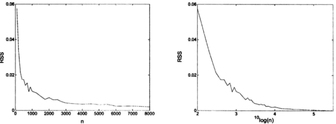
4-3. Accuracy of approximation as a function of the number of samples ... 75
4-4. Illustration of interpolation as a function of bin-width ... 76
5-1. Overview of sequential estimation ... 87
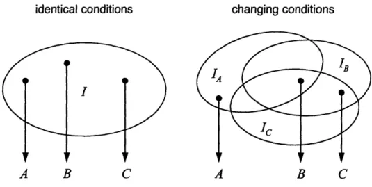
5-2. Experimentation as drawing data from a population defined by I ... 88
5-3. Overview of parallel estimation ... 88
5-4. Calculated/true relationship and synthetically generated measurements (o) ... 91
5-5. Simplified flow diagram of the Metropolis-Hastings algorithm ... 93
5-6. Determining the covariance matrix of the probing distribution ... 94
5-7. Trace and autocorrelation plots for the first MCMC simulation ... 94
5-8. Markov Chain traveling through the 2-D sample space of a and b ... 96
5-9. Example of a trace plot for a converged and not converged Markov Chain ... 96
5-10. Examples of the autocorrelation for a converged and not converged Markov Chain .... 97
5-11. Trace and autocorrelation plots after burn-in removal and thinning ... 98
5-12. Marginal posterior distributions for the parameters ... 99
6-1. Proposed framework for experimentation and estimation ... 102
6-2. Illustration of outlier identification ... 111
6-3. Illustration of incremental information gain ... 112
7-1. Prior distributions with uncertainty bounds ... 117
7-2. Typical objective function surface for a dataset generated in the absence of N2... 120
7-3. Concentration profiles (--- [N2]= l 014, -- [N2]=5 1014) ... 123
7-5. Sensitivity of [0(3P)] to the rate parameters (--- [N2]=-10 4, -[N 2]=5 10 )... 125
7-6. Typical temporal profile of a O(P) measurement ... 127
7-7. Strategy to estimate rate parameter kl with conventional estimation methods ... 130
7-8. Marginal posterior distribution for B compared to B for a particular data set ... 135
7-9. Comparisons of estimates for k, using the Bayesian and conventional approach ... 137
7-10. Evolving posterior probability distributions upon accumulating information ... 139
7-11. Posterior distributions for accumulated information ... 141
7-12. Variance and mean of p(k l ,...,yn) as a function of the number of data sets ... 142
7-13. Strategy to estimate rate parameter k, using the kinetic rate equations as model ... 144
7-14. Posterior probability distribution for rate parameter k2... 146
7-15. Validation of the k, estimate obtained with the kinetic model ... 150
7-16. Evolving variance of p(k lyl,... ,yn) for accumulating information ... 151
8-1. Concentration profiles ... 162
8-2. Forward reaction rates ... 163
8-3. Sensitivity of [C6H7'] to the rate parameters and equilibrium constant K2 ... 164
8-4. Measurements of optical density during reaction time ... 165
8-5. MCMC trace plots for the Global Dynamic Optimization scenario ... 169
8-6. Marginal posterior distributions for the Global Dynamic Optimization scenario ... 169
8-7. Objective function as a function of k4for k2ff401.0 and k3t=529.5 ... 170
8-8. Objective functions for the scenario of Global Dynamic Optimization ... 171
8-9. Model fit for various values of k4with k2f and k3f fixed ... 172
8-10. Marginal posterior distributions for rate parameters and diffusion limit ... 175
8-11. Model and data fit obtained from simultaneous data evaluation ... 176
8-12. Derived rate parameter k3f and ratio of forward rate parameters ... 177
D-1. Linear model including the 95% confidence interval bounds ... 210
D-2. Diagram describing the experimental design algorithm ... 212
D-3. Example of a search for the optimal experimental design using MCMC ... 213
E-1. Typical design of a tin oxide conductivity sensor (micrometer order of magnitude).. 223
E-2. Detection mechanism of chemiresistor sensors ... 223
E-3 Schematic of a CHEMFET sensor ... 224
E-4. Schematic representation of amperometric oxygen sensors ... 225
E-5. Cermet sensor front, back, and sideviews and blown up schematic ... 227
F-1. Simplified production rate curve and accompanying net cash flow ... 232
F-2. Overview of a reserves valuation by the DCF method ... 233
F-3. Schematic overview of the main resource categories ... 235
F4. Overview of reserves subcategories ... 236
F-5. The P90 estimate obtained from a normal probability and cumulative distribution .... 237
F-6. Comparison of the normal and lognormal distribution and their P90 values ... 242
F-7. Production profile of the PDP reserves and illustration of the VPP contract ... 245
F-8. Opportunity of including PDNP and PUD reserves into a VPP structure ... 246
F-9. Different degrees of uncertainty within proven reserves and the VPP risk definition. 247 F-10. Profiles for reserves A and B and production under the constraint of the VPP ... 250
F- . Optimal production schedule determined by simulation based optimal design ... 252
F-12. Probability distribution and contour plot of production levels as a function of time ... 253 F-13. Profile and contour plot for annual production evaluating PDNP and PUD reserves. 254
List of Tables
2-1l. Improving accuracy and precision by averaging measurements ... 36
5-1. Comparison of Bayesian and linear regression results ... 100
7-1. Mode and variance for the lognormal prior distributions ... 118
7-2. Comparison of summary statistics for rate parameter k ... 138
7-3. Comparison of summary statistics for the overall rate parameter (k2+k3) ... 146
7-4. Formulation of the Bayesian parameter estimation for k1 and k4... 147
7-5. Comparison of summary statistics for the overall rate parameter k ... 151
8-1. Incidence matrix for the system of case study 2 ... 160
8-2. Estimation results of Bayesian approach compared to Global Dynamic Optimization 168 8-3. Impact of evaluating multiple datasets on the estimate for k4... 176
E-1. Comparison between conventional analytical instruments and gas sensors ... 222
1
Introduction
If a man will begin with certainties, he shall end in doubts; but if he will be content to begin with doubts, he shall end in certainties.
Francis Bacon
1.1 Thesis Statement
When mathematical models are used to describe physical systems, inevitably approximations are made. The issue is not the introduction of uncertainties, as they will always be present, but to identify those that contribute most to the uncertainties in the predicted outcomes.
A typical example is the inevitable presence of uncertainties that arise from estimation of model parameters from experimental data. Unfortunately in practice uncertainty is often regarded as being disconnected from the quantities of interest and appears as supplementary information tagged onto deterministic results of a calculation or estimation.
There is a critical need for experimental design and parameter estimation procedures that reflect the underlying complexities of real systems. In particular, methods are needed that overcome the traditional limitations of Gaussian distributions to describe and propagate uncertainties.
The key premise of this thesis is that recent advances in Markov Chain Monte Carlo simulation methodologies can radically simplify the application of Bayesian statistics to reaction engineering problems.
The main contributions of this thesis are:
* A practical description of the Bayesian approach discussing concepts, advantages, computation, and practical implementation issues for applications and examples of interest to scientists and engineers.
* Illustrations of the intuitive evaluation of uncertainty according to the Bayesian approach.
* Illustrations of wide-spread misconceptions regarding conventional statistics related to erroneous applications in parameter estimation.
* The development of a general framework addressing experimentation and estimation that has four interdependent stages: system description, system analysis, experimentation, and estimation.
* A discussion and demonstration of mathematical tools, originating from system engineering, valuable for projects in experimentation and estimation.
* Identification of three parameter estimation strategies to be employed depending on the amount of data and the size of the parameters and variables to estimate.
* The development of tools to devise a stopping rule for a series of experiments and to discriminate among data for identifying outliers.
1.2 Motivation
A typical chemical reaction mechanism consists of multiple steps and species. Prediction of species concentration and dynamics requires knowledge regarding the kinetic rate parameters, stoichiometric coefficients, and initial conditions. These are usually estimated from experimental data. The estimation involves the combining of information from various sources, such as (1) concentration measurements as a function of time for one or more species involved in the reaction, (2) experimental conditions, such as
temperature, pressure, flow rates, and initial concentrations of reactants, and (3) existing knowledge on some or all of the kinetic rate parameters. Since in addition each type of information is characterized by uncertainty, the estimation problem mounts to a complex undertaking.
1.2.1 Complex Problems
Consider for example the reaction mechanism in Figure 1-1 of the relaxation of reactive
O(]D)
oxygen atoms, that has been proposed as part of a larger mechanism to understand stratospheric ozone depletion. The goal is to estimate the kinetic rate parameters k, from noisy experimental data.40 k,
O('D) +
N
2--
0(3P)
+
N
23
- 30O(
1D)
+
0
3-
20(
3P)
+
0
2 k M. k3r
O('D) + 03
->
202F
Io
100 ID k4 0( 3 ) +HeO('D) + He --> O3)+H
0 o t 1.5 time s x (o (a) (b)Figure 1-1. (a) First example of a reaction mechanism and (b) measurement results
With a reaction mechanism and data, such as shown in the example above, the main challenges to overcome in order to estimate the parameter k, are:
1. How to estimate the parameter k] from the data?
2. What factors contribute to the uncertainty in the value of k1?
3. How to combine various types of uncertain measurements and information? 4. How many experiments are required to sufficiently decrease the uncertainty?
5. How to combine the results from large amounts of data?
.. ' . . -J- -, .. . t I i i i
Though the case above involves an accepted reaction mechanism and thus strictly focuses on estimating a rate parameter, the example given in Figure 1-2 is not so straightforward. To resolve contradictions in the literature regarding the reaction mechanism of the addition of oxygen to the transient cyclohexadienyl radical, quantum mechanical calculations were performed to propose the mechanism given below. Subsequently, experimental data was generated by laser techniques with the goal of confirming this mechanism. 0.3
C6H,
- +
°2
/
p-C
6
H
7
00
'C
+2o-C + 6H
700
2o-C
6H
700
k4>
C6H6 + H0 2 012C
6H
7- k5 >products
0 1 2 3 4 time [ps] (a) (b)Figure 1-2. (a) Second example of a reaction mechanism and (b) measurement results
The challenges in the above example in estimating several rate parameters while attaining information regarding the proposed reaction mechanism are:
1. How to include existing uncertain estimates for particular rate parameters? 2. Which physical constraints can be applied to facilitate the estimation? 3. How reasonable is it to estimate multiple parameters from limited data?
4. How to implement different mechanism scenarios for the estimation in order to provide information regarding the applicability of the proposed mechanism?
5. How to combine the several estimates for a parameter obtained from different data
The examples above illustrate key questions that arise not only for this particular problem but for estimation problems in general. The central thesis of this work is a framework for experimentation and estimation based on Bayesian statistics.
1.2.2 Description of the Bayesian Approach
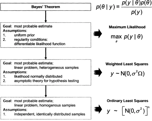
The Bayesian approach can be interpreted as a learning algorithm as specified according to the relatively straightforward Bayes' theorem, which is given by
p(Ol
y)
= p(yl
9)p(O)
(1-1)
P(Y)
where p(Oly) is the posterior probability distribution of the parameter 0, given the data y, p(yl ) is the likelihood function of the data, given the parameter 0, p(O) is the prior distribution, and p(y) is the probability distribution of the data y. Equation (1-1) effectively states that an initial parameter estimate described by p(O) is updated with information from new data y to the posterior estimate described by p(Oy).
The main advantages of applying the Bayesian approach are:
1. To have an intuitive estimation method based on unified underlying principles 2. To enable a consistent treatment of uncertainty incorporation and propagation 3. To evaluate uncertainty beyond 'normal' errors
4. To conveniently include multiple types of errors in the same problem 5. To robustly address multi-dimensional, nonlinear problems
6. To formally incorporate prior information
7. To have an explicit learning algorithm building on previous knowledge
These advantages of the Bayesian approach have previously been discussed in classical works arguing for Bayesian statistics [1, 2]. However, as only since recently the computational complexity resulting from the application of equation (1-1) to real life problems has been possible resolved, these advantages can now actually be attained. The
computational complexity referred to will become clear when considering that the total probability theorem to calculate p(y) becomes a multi-dimensional integral, as given by
p(0I y) = AyI)p( 0 ) d -. AY I O)p(O) (1-2)
J...
P(Y I)p(9)dO
1...d,,
where the vector 0 contains the collection of parameters 9l to 6n. The analytical solution of this multi-dimensional integral requires restricting assumptions to simplify the mathematics. Generally, in earlier works [1, 2] only Gaussian distributions were considered to characterize uncertainty, while mostly linear systems of a small number of parameters could be evaluated.
This thesis goes beyond the earlier works [1, 2] in relaxing such restricting assumptions by addressing the computational complexity through the use of Markov Chain Monte Carlo (MCMC) algorithms. MCMC simulation solves equation (1-2) by approximating the posterior p(0ly) through evaluating the product of the prior and likelihood function. The key realization that the denominator in equation (1-2) is merely a normalizing constant, leads to a problem formulation where non-Gaussian distributions can relatively easily be implemented in multi-dimensional nonlinear systems.
Though the MCMC algorithms require significant computational power, with the increased availability of faster and more powerful computers over the last decade practical applications of the Bayesian approach seem to become feasible in various disciplines. This is confirmed by Berger [3], who remarks the tremendous increase in activity, in the form of books, articles, or professional organizations, related to the Bayesian approach. Especially the last decade has seen an explosion of the number of publications.
1.2.3 The Relevance of Non-Gaussian Distributions
The uncertainty in model parameters will induce uncertainties in the model predictions. Even though uncertainty in the model parameters is often assumed to be characterized by the Gaussian distribution, the uncertainty in model outcomes is likely to be non-Gaussian. To illustrate this transformation of the probability distribution by uncertainty propagation through a model, consider a linear ordinary differential equation, such as a first order kinetic model, as defined by
d
dt
=
-ky(t)
k(1-3)
where k is the first order rate parameter, y is the species concentration at time t. Suppose that rate parameter k has been estimated and can be represented by the normal probability distribution N(/k,ak 2). With yo as initial concentration, solving the model analytically leads to
y(t) = y
e -(1-4)
so that concentration y can be predicted at a future time. Since the uncertain rate parameter k is now an exponential term, the uncertainty in concentration y is therefore represented by a lognormal distribution, as analytically can be derived as
)2 A k -^ _ 1 (In(y/yo)+tk )2
I__i
k/h)p(k)=
1
e
2/- : = p(y)= ye.
2 0/k(1-5)
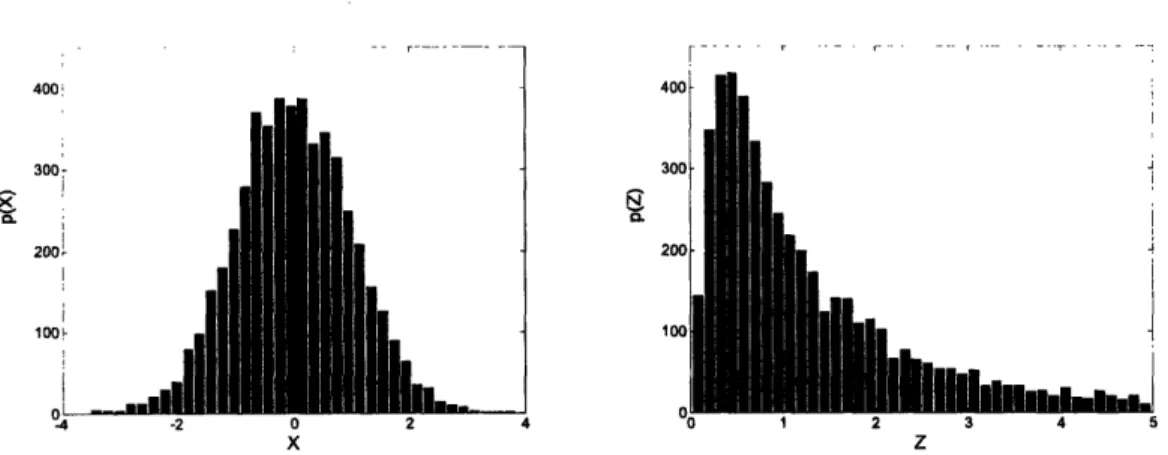
Alternatively, the transformation of a normal to a lognormal distribution can be illustrated by a Monte Carlo simulation. A standard normally distributed random variable X-N(O, 1) is sampled 5000 times, and each of these values is used to calculate random variable Z according to
after which the samples of Z are evaluated to approximate its probability distribution. Histograms representing the (non-normalized) probability distributions of X and Z are
shown in Figure 1-3.
IiL.
II
__ -2 0 2 4 3 -0 1 2 3 4 5 X ZFigure 1-3. Monte Carlo results illustrating the effect on uncertainty by variable transformation
As demonstrated by the simple example above, nonlinear models likely result in predicted values with their uncertainty characterized by non-Gaussian probability distributions. This effect is only exacerbated when dealing with large complex systems, and when the uncertainty of model input parameters or variables is already of a Gaussian nature. Nonetheless, conventional statistical methods generally ignore the non-normality and assume Gaussian distributions. The main reason is that the available mathematical tools are inapt for consistently propagating uncertainty of observables into uncertainty of the estimates. Regrettably, the average non-statistician is almost certainly not aware of the above discussion and the established, but incorrect approach has become to accept variances as provided by standard statistical software packages as the primary measure for the parameter uncertainty.
1.2.4 Acceptance of the Bayesian Approach
At first sight the methodology of the Bayesian approach appears to be rather involved compared to the conventional statistical methods that are easily accessible via standard statistical software packages. A closer look, however, reveals a surprisingly simple and intuitive concept for which the possibilities are virtually endless. However, to explore
400 300-200' ! i I lo-.. __ I ---- ' - I . 4 j 4 i i di
Bayesian interests beyond this initial barrier, the scientist or engineer should first realize the potential benefits of accepting the Bayesian approach. Unfortunately, the Bayesian literature explaining the concepts and principles of operation only illustrates applications involving relatively simple analytic or regression models. Applications of the Bayesian approach to complex engineering problems are still missing and they would be a welcome addition to the literature.
As a final note it is interesting to reiterate the opinion of Berger [3] regarding the future of statistics. According to Berger the language of statistics will be Bayesian, as this is significantly easier to understand and has been demonstrated to be the only coherent language to discuss uncertainty. On the other hand, from a methodological perspective, the Bayesian and Frequentist approaches can complement each other in particular applications, and thus at some point a unification seems inevitable.
1.3 Objectives
The primary objective of this thesis is to present tools based on Bayesian statistics that can aid scientists and engineers with experimentation and estimation. As a requirement, these tools should enable a convenient and consistent uncertainty evaluation, so that the impact of various sources of uncertain input on outcomes can be assessed. Additionally, the incorporation of information from various sources and of large amounts of data should be possible.
The secondary objective is to emphasize the importance of systems thinking regarding the estimation problem under investigation. Experimentation and estimation should be regarded as a learning process with feedback loops enabling multiple iterations to refine experiments and maximize information obtainable from the data. For example, theoretical understanding of the system contributes to the design of experiments, while also preparing the researcher for interpretation of data and identification of erratic results.
Subsequently assembled knowledge through experimentation can improve an understanding of the theory, thus shaping future experiments.
Since the acceptance and implementation of the proposed tools might be hindered by unfamiliarity with the Bayesian approach, the final objective is to describe the computational procedures in a clear and practical manner and to present the benefits of applying the Bayesian approach to case studies of complex engineering problems of interest to scientists and engineers.
1.4 Thesis Outline
This thesis has been organized around the proposed framework for experimentation and estimation and the linkages between the individual chapters are depicted in Figure 1-4.
Characterization of Uncertainty
(chapter 2) _Case Study 1
(chapter 7) Framework for
Bayesian Parameter Framework for
Approach Estimation Experimentation
(chapter 3) (chapter 5) and Estimation
t
(chapter 6) Case Study 2Cot (chapter 8)
Computation:
MCMC (chapter 4)
Figure 1-4. Schematic overview of the thesis structure
Chapter 2 sets the background of the thesis by discussing the interpretation of uncertainty and probability, common nomenclature, and definitions. Additionally, misconceptions and limitations resulting from conventional statistical methods are clarified before starting the discussion of the Bayesian approach.
Chapter 3 and 4 discuss the conceptual aspects, details, and computational issues regarding the Bayesian approach and Markov Chain Monte Carlo (MCMC).
Chapter 5 builds on various issues discussed in previous chapters by implementing the Bayesian approach to parameter estimation. This particular application will be described in detail and demonstrated through an example problem.
Chapter 6 introduces the proposed framework for experimentation and estimation. The discussion focuses on a structured approach to collecting essential knowledge regarding the system under investigation, and using that information towards experimentation and
estimation.
The background and theory discussed in the previous chapters are implemented through two case studies elaborately discussed in Chapter 7 and 8, which both demonstrate the merits of the proposed Bayesian framework for experimentation and estimation.
Finally, Chapter 9 and 0 discuss the conclusions and directions for future research, respectively.
2
Characterization of Uncertainty
The world as we know it seems to have an incurable habit of denying us perfection.
Peter L. Bernstein [4]
For a better understanding of uncertainty existing in realistic engineering problems, it is important to specify and clarify several notions that, though seemingly evident, are often misinterpreted. First, common attributes encountered in estimation under uncertainty will be defined to clarify the confusion attached to their colloquial use. Then, issues surrounding measurement errors will be explored in-depth, after which the limitations regarding uncertainty incorporation of conventional statistical methods are demonstrated.
2.1 Introduction
This section will define several terms commonly used regarding experimentation and estimation. In particular, the distinction between accuracy and precision and the distinction between error and uncertainty will be discussed.
2.1.1 Accuracy and Precision
In analyzing measurements, there is a clear need to make a distinction between the concepts of accuracy and precision, as illustrated in Figure 2-1. Suppose the center of the concentric circles represents the true value of the measurand, and a measurement in performed four times under apparently identical conditions.
accurate & precise accurate, not precise
Figure 2-1. Illustration of accuracy and precision
The accuracy refers to conformity of the measurements with the true value, thus how close they are to the center. In other words, accuracy is an indication for the quality of the measurement. The precision indicates the degree of perfection in the instruments and methods the measurement is obtained with and how reproducible the measurements are. In other words, precision is an indication for the quality of the operation with which the measurement is obtained.
2.1.2 Uncertainty, Error, and True Value
A suitable point to start this discussion is to state the definitions as recommended by the International Organization for Standardization (ISO) [5, 6]:
* Uncertainty:
"A parameter, associated with the result of a measurement, that characterizes the
dispersion of the values that could reasonably be attributed to the measurement."
* Error:
"The result of a measurement minus a true value of the measurand. "
* True value:
"A value compatible with the definition of a given particular quantity."
Though the concepts of uncertainty and error are clearly specified, the definition for true value is not very distinctive. In addition, the operational aspects for representing and handling uncertainty and error are not specified.
Various methods exist for representation and handling of uncertainty [7]. According to the Bayesian approach, uncertainty is characterized by probability distributions and propagated using the tools of probability theory. The true value of a quantity is still considered deterministic, fixed, but unknown, even though the degree of belief is expressed by a probability distribution and the quantity is manipulated as a random variable.
Finally, it is important to realize that uncertainty arises from various sources [5-8], such as systematic and random error, approximations and assumptions during estimation, linguistic imprecision regarding the definition of quantities, etc. The ISO guide identifies the following sources:
1. incomplete definition of the measurand
2. imperfect realization of the definition of the measurand
3. non-representative sampling - the sample measured may not represent the measurand
4. inadequate knowledge of the effects of environmental conditions on the measurement, or imperfect measurement of environmental conditions
5. personal bias in reading analogue instruments
6. finite instrument resolution or discrimination threshold
7. inexact values of measurement standards and reference materials
8. inexact values of constants and other parameters obtained from external sources and used in the data-reduction algorithm
9. approximations and assumptions incorporated in the measurement method and procedure
10. variations in repeated observations of the measurand under apparently identical conditions
Ideally each source of significance should be quantified, so that its contribution to the overall uncertainty in the system can be accounted for. However, in most cases only information regarding experimental error is available and taken into account. Since error
is such an important source for uncertainty, it will be discussed extensively in the following section.
2.2 Measurement Error
Experimentation is always subject to error. The Bayesian approach explicitly includes the measurement variance in the estimation, so an understanding of what actually is considered by 'measurement error' is important. Before actually considering the concept of measurement error in detail, the Central Limit Theorem and its importance for error statistics will be explained. Subsequently, the error model generally applied in parameter estimation is described and finally manipulation of the measurement error and data averaging are discussed.
2.2.1 Central Limit Theorem
The Central Limit Theorem [9] states that when Xi, X2,... is a sequence of independent identically distributed random variables with common mean / and variance
&
2, and when the random variable Z, is calculated asZ =
X
l+' ...
+ X -n
(2-1)
then the cumulative distribution function (CDF) of Zn converges to the standard normal CDF, defined by
X
2
CD(z)=
l
e dx (2-2)in the sense that
lim p(Z,, < z) = (D(z) (2-3)
According to this important theorem the realizations of the sum (or average) of a large number of random variables, independently generated from an identical distribution, will eventually be normally distributed. Besides the implicit assumption that both the mean and variance are finite, there is remarkably no other requirement for the distribution of Xi,
and thus any the distribution p(X) can be discrete, continuous, or mixed.
Random noise in many natural or engineered systems is considered to be the sum of many small, but independent random factors. The statistics of noise have empirically been found to be represented correctly by normal distributions, and the Central Limit Theorem provides the explanation for this phenomenon.
2.2.2 Random Error: Instrument Noise and Process Variability
Not considering systematic error, measurement error in experimental data can be considered composed of two different types of random error: (1) the instrument noise, and (2) the natural variability of the system, as schematically illustrated in Figure 2-2.
process variability E[data]
I
I'
instrument noise I I .-,<
~~~~~
>,
measurement errorFigure 2-2. Bisection of measurement error
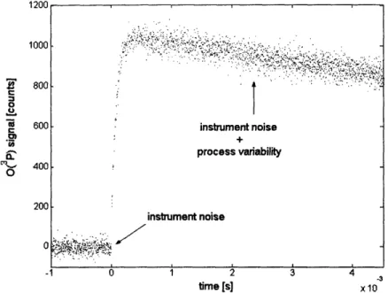
An example from actual data from Case Study (see Chapter 7) demonstrating the difference between instrument noise and measurement error is shown in Figure 2-3. The baseline signal (at t < 0) can be considered representative for the instrument noise, while
during the experiment (at t 0), the larger randomness in the signal combination of instrument noise and the inherent process variability.
1200 1000 800 0
-i
', 0 600 400 200 0 -1 0 2 time [s] 3 4 results from a -3 x10 Figure 2-3. Example of instrument noise and process variability2.2.3 Error Model
Combining the two sources of uncertainty discussed above, a measurement can be represented by
(2-4)
where yt is the observed value of yt, true at time t > 0, is the instrument noise, and is the process variability. For example e,, and can be specified as normally distributed random variables. Since normality is preserved upon linear transformations of normal random variables, the error model can be rewritten as
. = Y.- + o Yt f Vttrue ' - ~0 _
~~~~.:t,'..
'" · ! .' _ , ; , , > , . ;,.. I instrument noise process variability instrument noise .. . . ~.. (2-5) 1Y,
:,-- Y1,1rue, + 6" eVwhere Co is the total measurement error distributed according to co -N(O, ao2). Assuming
2
&E and , are independent normal random variables, the variance Uo2can be determined
from [2]
1 1 1
, - ;+ , (2-6)
o2
all o-;2where a 2 is the variance of the instrument noise and a 2 the variance of the process variability. Though en2 can be determined from baseline measurement, a2 will for most realistic situations be unknown. Therefore, the variance of the measurement error 0o2is considered unknown and will be included in the Bayesian parameter estimation.
2.2.4 Influencing Measurement Error
Of the two components of measurement error, the instrument noise can to some extent be controlled by e.g. the selection and correct tuning of the equipment, minimization of disturbances, etc. Beyond decisions regarding hardware selection and experimental setup, the effect of process variability can be decreased by measurement averaging, a feature
occurring in both Case Studies 1 and 2 (see Chapter 7 and 8). For example, each data point at time t shown in Figure 2-3 is determined by summing measurements (which is
equivalent to averaging in this context) at time t from several experiments.
Averaging has the useful characteristic that more accurate and precise data points are attained compared to the individual measurements. This effect is illustrated in Table 2-1, where the standard normal random variable Y is sampled n times to determine random variable Z as
y
+
1,+
Z Y
+
- + + ' (2-7)n
Table 2-1. Improving accuracy and precision by averaging measurements n E[Z] az 5 0.2561 0.1669 10 -0.0751 0.0975 20 -0.0666 0.0827 30 0.0312 0.0337 50 0.0123 0.0181 100 0.0018 0.0091 oo 0 0
The example shows that averaging an increasing number of samples n will improve both accuracy (Z -- E[Yi] = 0) and precision (z 2-> 0), as justified by the Strong Law of Large
Numbers [9]
Plim Y + Y2 +" '+ Yn = ) 1
(2-8)
n---°
n
where the mean of the standard normal distribution ,u = 0.
2.2.5 Systematic Error
Systematic error is a consistent error that is repeatable among multiple experiments. The only way to identify and quantify a systematic error is through comparisons with experimental results from different equipment or through calibration. Information on the possible existence is therefore necessary to account for systematic errors when analyzing the data, either with the proposed Bayesian approach or with any other statistical method. Nevertheless, as will be shown in Case Study in Chapter 7, the Bayesian approach facilitates a convenient intercomparison among estimation results visualizing any significant differences possibly caused by a changing systematic error. Such knowledge is extremely important to decide on the validity of the data and to recognize the undesirable influence of experimental settings, environmental effects, or other factors affecting experimentation.
2.3 Limitations of Conventional Statistics
This section will highlight some limitations and widespread misinterpretations of conventional statistical estimation methods. After illustrating the effect of approximations and transformations on uncertainty, standard error propagation is discussed. Finally, the justification that the uncertainty of a parameter estimate is always normally distributed when averaging over sufficient number of data points, is shown to be based on a misconception.
2.3.1 Linear Error Statistics
A general linear model with only two parameters is specified as
y, = a + bx +
(2-9)
where yi is the dependent variable for i = 1,...,n data points, xi the independent variable, a and b are the intercept and slope, respectively, of the linear model, and e is the error term which is normally distributed according to e -N(0, 2) with zero mean and unknown
variance a:. An equivalent, but more general notation is
y = X (2-10)
where ,8 is the parameter vector and X is the design matrix, in this case given by
1 Xi
x2
X = I x2 (2-11)
/) = (XIX)' X
Ty
(2-12)the sample variance s2, which is an unbiased estimator for the unknown variance a2, can be calculated from the residual sum of squares according to
2
____
2
s2
(Yi - (a +bx
(2-13)n-k-1
=--for n data points and k independent variables. The estimates 6-a2 and -f2 of the variances of a and b are the diagonal elements of covariance matrix X, which can subsequently be determined as
~~~~~~~~~~2
a j= s2(XTx)- (2-14)
ab i
2.3.2 Nonlinear Approximations
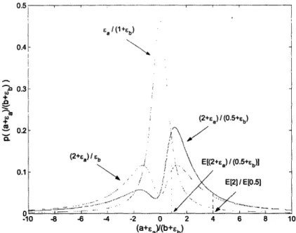
Though equation (2-14) is derived for linear systems [10], it is often similarly applied for nonlinear models by approximating the nonlinearity with a Taylor series expansion, of which only the linear terms are retained. The following example [8] clearly shows that the sensitivity of the nonlinear model output to uncertain input parameters should not be underestimated. In addition, it demonstrates that the uncertainty in the model output only can be properly characterized by the full probability density function to be obtained by evaluating the complete model, and not an approximation.
We are interested in evaluating the ratio of two random variables A and B. Such calculation occurs in a variety of applications, e.g. to calculate speed when measuring distance and time, or to determine equilibrium constants in chemical reactions. To evaluate this system, the model is defined as
f(A,B)
=
+
af(
)
E)(2-15)
B
b+eb
where a and b are non-negative constants, and a and eb are independent random variables distributed according to the standard normal distribution N(tu,2) = N(0,1), with
N(0,1) = (z) =- e 2 (2-16)
The common misconception is that the probability density function for the function J(E, , b) is normally distributed as well. However, the analytical expression for this
probability density function is given by
a2+b2
=~q
=
1 +
w
Er
i
h
b=1+at
2(a
([(t)
ea)
Ef(
qfi
1
with
=b+at
(2-17)
tb
+ 6b
)(l+ t
2)
0(q) 2
,2
Obviously, the calculation of the mean OfJ(sa, eb) by the ratio of the expected values of a and b is likely to be incorrect. More formally
a
1
E[a]Ea~e
= tD(t)dt E•
a
]
[b +
]eb
J
tOt
E[b]
(2-18)
further supporting the statement that uncertainty should be incorporated at the start of a problem and propagated while solving a problem. The final solution should be obtained
by evaluating the full probability distribution.
For a clear illustration that uncertain input can have a significant effect on the outcome of a problem, the probability density functions for three combinations of the constants a and b are shown below in Figure 2-4. Depending on the values of a and b the distribution can
exhibit unimodal symmetric behavior, bimodal symmetric, or even bimodal asymmetric behavior. 0. 0. 0. 4 3 2 1 O. -10 -8 -6 -4 -22 0 (a+%)y(b+ b) 4 6 8 10
Figure 2-4. Probability density functions for (a+ed/(b+sb)
2.3.3 Error Propagation
A possible representation of the uncertainty in the outcome y of a calculation as a function of the uncertainty in the independent variables can be attained by error propagation. The two basic rules in error propagation are as follows [ 11]
y = x + z-(u + w)
x-z
y=
u W= y=6x +6z + 6u +56w
by _ Sx z Tu w Yl IxI +STl- IU wlwhere & represents the uncertainty in the corresponding variable i. In the special case that the variables are independent and normally distributed, error propagation can be calculated as + en AWM A a / (1+E) ; (2+Sa) / (0.5+eCb) ~~~~~~~!,
'
!\'/
(2+Sa)/Sb / E[(2+£a)(O.5+) El2] EO.51 ... / . ... (2-19) (2-20) 0.5-, _ ___ _-n -- , - --- I - . --- --.- I , - . I . I 2V =x+z-(U
+
w)
X'Z '= U *W =:>6y
= 4(6X)2 + (5z)2 + (Stu)2 + (gW)2jYI
V C IX T+
(+
( FJ ±(WWhen the uncertainty i is represented by the standard deviation oi, equation (2-22) can be derived as follows. Consider the general model denoted as
y(x) = f (x1, x2, ..., Ixn) (2-23)
and approximate y(x) by a Taylor series expansion. By using the following properties of expectation operators [9] when Z = aP + b
E(Z) = aE[P] + b
(2-24) Z2 2 p2
o7Z = ao17
where Z and P are random variables, and a and b are given scalars, the total variance ay2
can be calculated from the individual variances of xi as
/ 2 2
ax
1) ax2)
2
2
+
+
'
(
,x)
,
r
.
2
+ covariance terms +-.-X2 Vax,,)
When the covariance between the independent variables xi can be neglected, the desired equation is obtained. This can be illustrated with the following example. Consider the system model y(x) = xx2x3 y _ ' XX3 ; ax, (2-26) "y = X X oy 3 ; = .1X, aX2 ax3 (2-27) (2-21) (2-22) (2-25) so that
and assuming that the parameters are uncorrelated, then
a
= (x2x3)2o + (xx 3)2Cr: + (x x,) 2o (2-28)which can be rewritten as
(xl1I+
I.
(
;+
(2-29)
(xIx2x3)2 X, x2 X3
leading to
__Y
ax.
+
ax,
+(.2LJ
(2-30)IYI
2(X,
X2 ) (X3 )(-0which is the quadrature summation given in equation (2-22) that is applicable to error propagation for a system model as given in equation (2-26).
Though quadrature summation is a convenient approximation of uncertainty propagation, the mathematical manipulations include some assumptions and, more importantly, full probability distributions are not considered. Therefore, though applicable to both products and quotients, equation (2-22) can never represent the situation as discussed in Section 2.3.2, where possible probability distributions of a quotient of two normally distributed variables were considered (see Figure 2-4).
2.3.4 Abuse of the Central Limit Theorem
As inference in data analysis usually produces average estimates over series of experimental data, the common misconception is that the uncertainty of the parameter is normally distributed. This misconception has its origin in the confusing terminology of conventional statistics.
According to conventional statistics the 'true' value of a parameter 0 is considered fixed, the 'statistic' s is introduced to account for the random effects of experimentation (more on this below in Section 3.2.1). This statistic 9, which is a random variable representing the unknown parameter 0, is merely a point estimate. When each experiment is considered as an independent random draw from the population of 9, then its expected value E[ ] can, at a sufficiently large sample size, be considered normally distributed according to the Central Limit Theorem (see Section 2.2.1).
The misconception is then to assume that the statistic is normally distributed. However, bear in mind that while the estimation result E[ ] is likely normally distributed, the statistic can be distributed according to any probability density function, while the
parameter 0 is fixed and thus not distributed at all.
The above discussion is illustrated by the following example. Suppose that a sequence of random variables Y is drawn from a particular distribution p(Y), yet to be defined. The statistic 9 can be considered equivalent to the random variable Yi. Subsequently, random variable Z is calculated by applying equation (2-7), repeated here for convenience
Z
= Y Y2 +.. + + Y (2-7)n
so that the distribution p(Z) becomes approximately normal for sufficiently large n. The expected value E[ ] is equivalent to the normally distributed random variable Z.
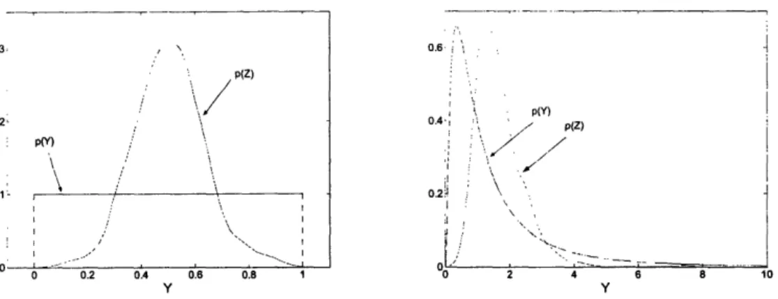
Figure 2-5 shows the distributions p(Y) and p(Z) for the cases of sampling Y from a uniform and a lognormal distribution, for n = 10. The probability distributions p(Y) are plotted exactly, while the probability distributions p(Z) are obtained from a kernel density estimate of 500 samples for Z and are thus the result of 500 10 draws of Yi.
3, \ p(Z) / / \/ 2 P ),' \ '\ # / ,. 1 - ,'' OA
~;
\ I ----: I o 0.2 0.4 0.6 0.8 1 Y 0.6 . 4'1~~~~~~~~' .:' ; 2 I o.4~ ', , P(Z). ;m .' . t ,l ' ', . .:- - - . . . I_-:... 0 2 4 6 8 10 YFigure 2-5. Illustrations of the Central Limit Theorem
Conventional estimation methods only provide the expected values of point estimates
E[ 9 ], which indeed can be considered normally distributed. However, typically the
normally distributed E[ ] is mistaken for the statistic 09, which is subsequently also considered to follow a normal distribution. As seen in the example above though, this does not have to be the case at all.
3
The Bayesian Approach
Inside every Non-Bayesian, there is a Bayesian struggling to get out.
Dennis V Lindley
When dealing with uncertain systems, incorporation of the uncertainty at the stage of problem formulation and uncertainty propagation throughout the problem-solving process
is important. The Bayesian approach is a powerful method based on unified underlying principles accomplishing a consistent treatment of uncertainty. After a review of the roots of probability theory and some conceptual issues regarding plausible reasoning, three definitions of probability theory, Classical, Frequentist, and Bayesian, the characteristics of the Bayesian approach, and some application issues will be described in more detail. Finally, the relationship of the Bayesian approach with common alternative estimation methods will be illustrated.
3.1 Introduction
A variety of topics are briefly discussed to introduce the conceptual framework of the Bayesian approach that forms the core of this thesis. A note on uncertainty is followed by a discussion on plausible reasoning and induction, and an explanation how the Bayesian viewpoint fits to all of this.
3.1.1 Inescapable Uncertainty
We can never have complete knowledge regarding phenomena under investigation. Solving problems, being it in engineering or any other field, will always be plagued by
uncertainty originating from various sources [7, 8]. Our models are an approximation of reality, data is collected from inherently variable systems, the measurement equipment introduces additional error, etc. The generally accepted language to quantify uncertainty is probability theory. Probability can be interpreted as "the degree of uncertainty, which is to the certainty as the part to the whole." This very early definition by Bernoulli echoes the more recent Bayesian perspective on probability and will be applicable throughout this thesis.
3.1.2 Reasoning
The first recorded activity in the field of probability theory originates from the gambling tables of the 16th century. Realizing that though the future could not be predicted, the
limited number of possible outcomes of a certain game allowed the reasoning about the best bet to place, in other words about the best decision to make with minimal risk. This type of reasoning is based on deductive logic, schematically shown in Figure 3-1 [12], and though professional gamblers can attest to its usefulness, applications to realistic problems in science and engineering are rather limited.
deductive logic: pure math inductive logic: plausible reasoning
effects effects possible or outcomes causes outcomes effects or observations
Figure 3-1. Deductive and inductive logic
Bernoulli's theorem, also known as the Law of Large Numbers, was the first formal account in calculating probabilities. Identifying the distinction between frequency and probability, the Law of Large Numbers relates the probability of occurrence in a single trial to the frequency of occurrence in a large number of independent trials. Bernoulli also posed the inverted problem of what can be said about the probability of a certain event after observing the frequency of occurrence of this event. This kind of question is
![Table 2-1. Improving accuracy and precision by averaging measurements n E[Z] az 5 0.2561 0.1669 10 -0.0751 0.0975 20 -0.0666 0.0827 30 0.0312 0.0337 50 0.0123 0.0181 100 0.0018 0.0091 oo 0 0](https://thumb-eu.123doks.com/thumbv2/123doknet/14054325.460577/36.918.229.665.126.366/table-improving-accuracy-precision-averaging-measurements-e-z.webp)