Publisher’s version / Version de l'éditeur:
Pure and Applied Chemistry, 90, 2, pp. 395-424, 2018-01-04
READ THESE TERMS AND CONDITIONS CAREFULLY BEFORE USING THIS WEBSITE.
https://nrc-publications.canada.ca/eng/copyright
Vous avez des questions? Nous pouvons vous aider. Pour communiquer directement avec un auteur, consultez la première page de la revue dans laquelle son article a été publié afin de trouver ses coordonnées. Si vous n’arrivez pas à les repérer, communiquez avec nous à [email protected].
Questions? Contact the NRC Publications Archive team at
[email protected]. If you wish to email the authors directly, please see the first page of the publication for their contact information.
Archives des publications du CNRC
This publication could be one of several versions: author’s original, accepted manuscript or the publisher’s version. / La version de cette publication peut être l’une des suivantes : la version prépublication de l’auteur, la version acceptée du manuscrit ou la version de l’éditeur.
For the publisher’s version, please access the DOI link below./ Pour consulter la version de l’éditeur, utilisez le lien DOI ci-dessous.
https://doi.org/10.1515/pac-2016-0402
Access and use of this website and the material on it are subject to the Terms and Conditions set forth at
Interpreting and propagating the uncertainty of the standard atomic
weights (IUPAC Technical Report)
Possolo, Antonio; Van Der Veen, Adriaan M. H.; Meija, Juris; Hibbert, D.
Brynn
https://publications-cnrc.canada.ca/fra/droits
L’accès à ce site Web et l’utilisation de son contenu sont assujettis aux conditions présentées dans le site
LISEZ CES CONDITIONS ATTENTIVEMENT AVANT D’UTILISER CE SITE WEB.
NRC Publications Record / Notice d'Archives des publications de CNRC:
https://nrc-publications.canada.ca/eng/view/object/?id=f1f2ca7f-9b5f-4da0-bbba-d196cc190911 https://publications-cnrc.canada.ca/fra/voir/objet/?id=f1f2ca7f-9b5f-4da0-bbba-d196cc190911IUPAC Technical Report
Antonio Possolo*, Adriaan M. H. van der Veen, Juris Meija and D. Brynn Hibbert
Interpreting and propagating the
uncertainty of the standard atomic weights
(IUPAC Technical Report)
https://doi.org/10.1515/pac-2016-0402
Received April 1, 2016; accepted October 10, 2017
Abstract: In 2009, the Commission on Isotopic Abundances and Atomic Weights (CIAAW) of the International
Union of Pure and Applied Chemistry (IUPAC) introduced the interval notation to express the standard atomic weights of elements whose isotopic composition varies significantly in nature. However, it has become apparent that additional guidance would be helpful on how representative values should be derived from these intervals, and on how the associated uncertainty should be characterized and propagated to cognate quantities, such as relative molecular masses. The assignment of suitable probability distributions to the atomic weight inter-vals is consistent with the CIAAW’s goal of emphasizing the variability of the atomic weight values in nature. These distributions, however, are not intended to reflect the natural variability of the abundances of the dif-ferent isotopes in the earth’s crust or in any other environment. Rather, they convey states of knowledge about the elemental composition of “normal” materials generally, or about specific classes of such materials. In the absence of detailed knowledge about the isotopic composition of a material, or when such details may safely be ignored, the probability distribution assigned to the standard atomic weight intervals may be taken as rectan-gular (or, uniform). This modeling choice is a reasonable and convenient default choice when a representative value of the atomic weight, and associated uncertainty, are needed in calculations involving atomic and relative molecular masses. When information about the provenance of the material, or other information about the isotopic composition needs to be taken into account, then this distribution may be non-uniform. We present several examples of how the probability distribution of an atomic weight or relative molecular mass may be characterized, and also how it may be used to evaluate the associated uncertainty.
Keywords: atomic weights; atomic-weight intervals; beta distribution; delta scale; delta value; fractionation;
Gaussian distribution; interval arithmetic; measurement uncertainty; normal; probability distribution; rec-tangular distribution; relative molecular mass; standard atomic weight; uncertainty; uncertainty propaga-tion; uniform distribution.
1 Introduction
At its 2009 meeting in Vienna, the IUPAC Commission on Isotopic Abundances and Atomic Weights (CIAAW) resolved to express the standard atomic weight of ten elements – including hydrogen, carbon,
Article note: Sponsoring body: IUPAC Inorganic Chemistry Division.
*Corresponding author: Antonio Possolo, National Institute of Standards and Technology (NIST), Gaithersburg, MD, USA, e-mail: [email protected]
Adriaan M. H. van der Veen: Van Swinden Laboratorium (VSL), Delft, The Netherlands Juris Meija: National Research Council Canada (NRC-CNRC), Ottawa, ON, Canada D. Brynn Hibbert: UNSW Sydney, Sydney, NSW, Australia
and oxygen – by means of intervals that characterize the span of their atomic-weight values in so-called “normal” materials.
We use the term “atomic weight” interchangeably with, and as shorthand for “relative atomic mass”, consistently with the historically customary usage recognized in the IUPAC Green Book [1, 2.10(8),6.2].
The CIAAW defines “normal” material as any terrestrial material that “is a reasonably possible source for this element or its compounds in commerce, for industry or science; the material is not itself studied for some extraordinary anomaly and its isotopic composition has not been modified significantly in a geologi-cally brief period” [2]. Concerning the provision that the isotopic composition of a “normal” material should not have been modified significantly in a geologically brief period, John Böhlke (2015, personal communica-tion) has pointed out that “high and low atomic weight values of light elements commonly are due to isotopic fractionation processes that are happening every day,” as arise in respiration, evaporation, and dissolution.
The CIAAW explained that expressing the standard atomic weights as intervals serves to emphasize that the atomic weights are not constants of nature [3–5]. This choice was reaffirmed when the CIAAW published the 2011 version of the atomic weights, and added bromine and magnesium to the list of elements whose standard atomic weights are expressed as intervals [6]. The same approach has been used in the 2013 version of the standard atomic weights [7]. The 2009 recommendation to use interval notation did achieve the valu-able educational goal of drawing attention to the fact that isotopic composition can vary among natural materials, hence so do the atomic weights [8].
The expression “constant of nature” is used informally, generally referring to values of properties of natural entities or processes that are believed to remain invariant in time and space. Examples include
ma(11B), the atomic mass of 11B, and the Newtonian gravitational constant G. According to Audi et al. [9],
ma(11B) = 11.009 305 4 Da, where 1 Da = m a(
12C)/12 = 1.660 539 040 × 10−27 kg is the unified atomic mass unit [10].
The relative atomic mass of this isotope, Ar(11B) = m a(
11B)/(m a(
12C)/12) = 11.009 305 4, and the relative atomic
masses of all the other isotopes, are believed to be constants of nature.
The atomic weight of element E in material P is a weighted average of the relative atomic masses of the element’s isotopes present in material P, where the weights (of this weighted average) are the amount frac-tions of the isotopes of element E in material P [5]. Therefore, the atomic weight of element E is a collective property of the set of isotopes of E in material P that depends on the isotopic composition of material P, hence typically will have a different value in different materials.
1.1 Expressions of uncertainty for atomic weights
Because the atomic weight of an element in a material depends on the isotopic composition of the material, in the absence of specific knowledge about this isotopic composition the uncertainty surrounding an atomic weight usually is much larger than the uncertainty surrounding an isotopic mass. For example, the stand-ard uncertainty (1σ) associated with the isotopic mass of 11B is u(m
a(
11B)) = 0.000 000 4 Da [11, table I], hence
the isotopic mass of 11B is known to better than 0.04 parts per million. However, boron has standard atomic
weight [10.806, 10.821], indicating that the atomic weight of boron in a generic “normal” material is known to no better than 0.7 parts per thousand.
The 2009 Technical Report prepared by the CIAAW did not offer guidance on the practical use of the new interval notation [5]. The present Technical Report illustrates how the standard atomic weights may be interpreted probabilistically, how such interpretation may be used in uncertainty evaluation, and how the uncertainty associated with the atomic weights may be propagated to relative molecular masses and to other quantities that depend on the atomic weights.
IUPAC’s 1951 report on the Standard Atomic Weights for the first time included a reference to uncertainty, recommending the standard atomic weight of sulfur as 32.066 ± 0.003 [12]. The CIAAW explained in 1951 that the “±0.003” represents the range of the atomic-weight values of sulfur due to natural variations in the abun-dance of its isotopes [12]. Coplen and Peiser [13, 14] discuss the use of uncertainties in this context, and their interpretation. By 1969, standard atomic weights were qualified with uncertainties [15].
Guide to the expression of uncertainty in measurement (GUM) [16], and they were understood as follows: “any
user of the atomic-weight data would, with high probability, find the atomic weight of any element in any normal sample to be in the range indicated by the uncertainty for the recommended standard atomic weight” [6, Page 1048].
For all the other elements, Meija et al. [7, table 1] give the standard atomic weight as a single value quali-fied with a decisional uncertainty that is conventionally denoted using a parenthetic notation. For example, the standard atomic weight of molybdenum is 95.95(1) [7], which means that Ar(Mo) = 95.95 and that the asso-ciated decisional expanded uncertainty is U[Ar(Mo)] = 0.01. In general, the interval from Ar(E) − U[Ar(E)] to
Ar(E) + U[Ar(E)] is believed to encompass the atomic weight values of element E in essentially all “normal” materials.
Molybdenum is one of several elements that have two or more stable isotopes whose relative abundances are known to vary among “normal” materials, but whose variability does not exceed the evaluated measure-ment uncertainty of the atomic weight derived from the best measuremeasure-ment of the isotopic abundances of the element. For elements in this category (and indeed for all elements in categories 2–5 as defined in Section 1.4 of Wieser et al. [6]), the decisional uncertainty U[Ar(E)] is given in parentheses following the last significant figure to which it is attributed.
It should be noted that the interval notation expresses the same sources of uncertainty, and has the same general meaning as the conventional, parenthetic notation. However, the interval indicates that the variablity of the atomic weight in “normal” materials is the dominant source of uncertainty, whereas the parenthetic notation indicates that other sources of uncertainty dominate. The interval notation also avoids suggesting a particular value as possibly being the “best estimate” of the atomic weight. The CIAAW determines whether a particular element belongs in one category or the other based on published information and on the CIAAW’s best judgment, similarly to how the CIAAW determines whether each atomic weight should be qualified by a particular footnote (“g”, “m”, or “r”). Therefore, the result of such determination may change over time, from one release of the atomic weights to the next.
The standard atomic weight values for elements like molybdenum are obtained by averaging experi-mental results obtained from many samples, hence the variations in isotopic compositions are incorporated automatically, yet measurement uncertainty currently still is at least as large as these natural variations. And molybdenum, in particular, currently has its atomic weight qualified with a footnote “g”, indicating that “geological materials are known in which the element has an isotopic composition outside the limits for normal material”, and that “the difference between the atomic weight of the element in such materials and that given in the table may exceed the stated uncertainty” [7, table 1].
It should be noted that the aforementioned decisional expanded uncertainty differs essentially from the “expanded uncertainty” defined in the GUM, where an uppercase U is also used to denote the latter. Accord-ing to the GUM (2.3.6), the expanded uncertainty is a multiple of the combined standard uncertainty, the multiplier (coverage factor) being chosen so that the interval centered at the estimate of the measurand, and of half-width equal to U, is believed to include the true value of the measurand with a specified probability.
From 2009 onward, the standard atomic weights of selected elements have been specified in such a way that the corresponding intervals are intended to encompass measured atomic weight values in all “normal” materials, both when the intervals are given explicitly (for example, [10.806, 10.821] for boron, which does not identify any particular value within this interval as “best” in any sense), or implicitly as a single value qualified by the associated uncertainty (for example, 40.078(4) for calcium, which is equivalent to [40.074, 40.082] except that it gives 40.078 as the “best” estimate).
The CIAAW derives these intervals by pooling the expert knowledge of its members taking into account the published information about isotopic abundances, in what effectively is an informal elicitation exercise [17].
In this conformity, when probability distributions are employed to describe states of knowledge about the values of the atomic weights, it is acceptable to assume that the distributions are essentially concentrated either in the standard atomic weight intervals, or in the intervals that are specified implicitly using the paren-thetic notation. “Essentially concentrated” means that the probability is either zero or very close to zero that any “normal” material will have atomic weight outside of the standard atomic weight interval [6].
A concise (parenthetic) notation for uncertainties has a long history, but it has been interpreted differently in different contexts. For example, CODATA [10] has adopted the concise form 1.660 539 040(20) × 10−27 kg to
express the value of the (unified) atomic mass constant mu and its associated uncertainty. In this case, the digits between parenthesis specify the standard measurement uncertainty (sometimes described informally as a “1σ” uncertainty), u(mu) = 0.000 000 020 × 10−27 kg, not an expanded uncertainty. The probabilistic
inter-pretation of 1σ uncertainty is commonly made by reference to a Gaussian distribution, hence, and in this case, suggesting that the true value of mu lies within u(mu) of the estimate of mu published by CODATA with approximately 68 % probability.
The uncertainties reported by the CIAAW, using this parenthetic notation or any other, for the atomic weights and isotopic abundances, are expanded uncertainties corresponding to several different values of the coverage factor or of the coverage probability. Since some uncertainty statements, for example result-ing from Monte Carlo uncertainty evaluations, do not involve application of coverage factors, a comparably effective, and indeed preferable alternative characterization consists of specifying the coverage probability. However, neither the assignment of values to the standard atomic weights, nor the evaluations of their asso-ciated uncertainties, are within the scope of this contribution: Meija and Possolo [18] describe a rigorous framework for the corresponding calculations.
In all cases, the important requirement to satisfy is that the probability assigned to particular intervals – be they standard atomic weights that are expressed as intervals, or coverage intervals generally – should be stated explicitly whenever intervals are reported that have a probabilistic interpretation, to remove all ambi-guity and to ensure comparability of results. When, for example, the intention is to state that the probability is zero for values outside of an interval of finite length, then a probability distribution with correspond-ingly bounded support will have to be used, for example rectangular, triangular, rescaled and shifted beta (reviewed in §5.3, following the description of Algorithm S), etc.
If a distribution with unbounded support is used, for example a Gaussian (or, normal) distribution, then its standard deviation will have to be tuned so that the distribution assigns the intended probability to the interval in question, and this probability should be stated explicitly.
The expression of standard atomic weights using interval notation has emphasized the variability of the atomic weights in nature, while also capturing the measurement uncertainty associated with delta values (reviewed in §4) and with the relative atomic masses of the isotopes [6, Page 1053]. Such intervals were con-ceived as notational and educational devices, not as computational tools. However, this was achieved at the expense of deemphasizing the actual form of the underlying dispersion of values and how to use it in practi-cal practi-calculations.
To characterize the uncertainty associated with a standard atomic weight expressed as an interval, it is necessary to specify a probability distribution on the interval: this distribution may be uniform (or, rectan-gular), or it may be some other distribution. The incomplete knowledge that this distribution reflects may be dominated by measurement uncertainty, as it is for tellurium, or its principal source may be ignorance about the origin of the material, as it is for lithium. The same applies to the full characterization of the uncertainty associated with an atomic weight expressed using the parenthetic notation.
1.2 Notational conventions
We have adopted the following notational conventions, which are generally consistent with the guidance provided in the IUPAC Green Book. We note that different notation has been used in recent IUPAC Technical Reports, and that the current IUPAC Recommendation on definitions of terms relating to mass spectrometry [19] does not address several of the topics mentioned here.
– Ar,P(E) denotes the atomic weight (relative atomic mass) of element E in material P. For example,
Ar,SEAWATER(B) denotes the atomic weight of boron in seawater.
– Ar(E) denotes the atomic weight of an element or isotope E disregarding the provenance of the element, hence effectively averaged over all “normal materials”. For example, Ar(H) = [1.007 84, 1.008 11], and
Ar(Mo) = 95.95(1) [7]. When E designates an isotope, Ar(E) is invariant across all materials. For example,
Ar(16O) = 15.994 914 619 566(179) [11, table A].
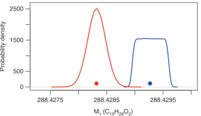
– Mr,P(S) denotes the relative molecular mass of substance S as it occurs in material P. For example, in §6.4 we compute Mr,HUMAN(TESTOSTERONE) = 288.4289, but also refer to it as the value of a random vari-able MH whose probability distribution we use as a model for the associated uncertainty. The subscript P generally may be any string that denotes the relevant material: for example, in §4.3 we use “C” in this role because several quantities that we consider there pertain to a sample of colemanite.
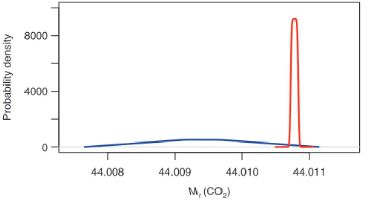
– Mr(S) denotes the relative molecular mass of substance S disregarding the provenance of the material containing the substance. For example, in §6.1 we compute Mr(CO2) = 44.009 40.
– xP(S) denotes the amount fraction of substance S in material P, where S may be a molecule, element or isotope. For example, xSRM951(10B) denotes the amount fraction of the isotope 10B in NIST Standard
Refer-ence Material (SRM) 951.
– wP(S) denotes the mass fraction of substance S in material P, where S may be a molecule, element or isotope. For example, in §2 we conclude that
2
H O(O) 0.888 083, 0.888 114 .
w =
– NP(S) denotes the number of entities S in material P. For example, NAVO28-S5(28Si) denotes the number of 28Si
atoms in silicon sphere AVO28-S5 [20].
– RP(iE/jE) denotes the isotope-number ratio (also called isotope ratio) for isotopes iE and jE in
mate-rial P: that is, NP(iE)/N P(
jE). Isotope ratios are discussed and used in §4. For example, the isotope ratio
RVSMOW(18O/16O) in the Vienna Standard Mean Ocean Water (VSMOW) is used in Listing 2.
– The delta value δSTD,P(iE/jE) (where by convention iE is the heavier isotope and jE is the lighter one) denotes
the relative difference of isotope ratios for a particular pair of isotopes of element E in material P and in a standard or reference STD (§4): RP(iE/jE)/R
STD(
iE/jE) − 1.
Note that, in the notation that we adopt, the first (or only) subscript affecting the Greek letter δ designates the standard or reference. For example, δSRM951,SEAWATER(11B/10B) = + 39.5 ‰ [21, Page 15]: this means that the isotope
ratio RSEAWATER(11B/10B) is 1.0395 times larger than its counterpart for NIST SRM 951.
When an element has only two stable isotopes, occasionally we abbreviate the delta notation and mention only the heavier isotope. For example, in §3, where we state that δLSVEC(7Li) ranges from −10 ‰ to
+56 ‰ among marine sources [21, table 5].
1.3 Overview
In Section 2 we review difficulties that the adoption of the interval notation has created for many users of the atomic weights, and discuss the limitations of an approach using interval arithmetic, which we therefore discourage. We believe that a probabilistic approach to the interpretation and use of the interval notation will be more useful than interval arithmetic, and that it will also be better aligned with the motivation for adopting the interval notation. Also, a probabilistic interpretation is consistent with the characterization of uncertainty promoted by the GUM.
In Section 3 we review the concept of uncertainty when it is applied to standard atomic weights, and its expression and interpretation. This serves as preparation for the illustrations provided in Section 5 of how the knowledge about the dispersion of isotopic compositions may be modeled probabilistically, followed by a discussion of how such models may be used to evaluate the uncertainty of relative molecular masses and of other quantities that depend on the values of the atomic weights.
In Section 4 we review the delta scales and notation commonly used to express relative differences in isotopic abundances, and show how, based on these scales, values and associated uncertainties can be obtained for atomic weights.
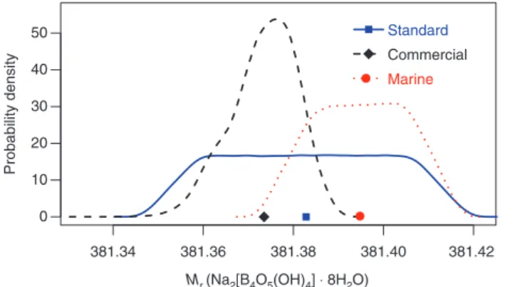
We provide an example of the evaluation of measurement uncertainty for the relative molecular mass of borax (Section 6), which shows that the choices the CIAAW has made regarding the standard atomic weights can co-exist with uncertainty characterizations, and that such co-existence: (i) on the one hand, satisfies the
desideratum of the CIAAW to increase awareness about the natural variability of atomic weights; and (ii) on the other hand, also satisfies the practical requirements of those users that need to treat measurement results involving the atomic weights consistently with the provisions of the GUM.
2 Interval arithmetic
The interval notation is challenging for many users of the atomic weights because virtually all compu-tations in science and technology involve single numbers, and neither intervals nor any other sets of numbers.
The question naturally arises of whether calculations involving the standard atomic weights (expressed as intervals) should be performed according to the rules of interval arithmetic, whose results also are intervals. Interval arithmetic has been used to bound rounding errors in mathematical computation, for uncertainty analysis, and for optimization [22]. For example, short of employing interval arithmetic, it is not obvious how to calculate the standard relative molecular mass of H2O or how to obtain the ratio of the standard atomic weights of oxygen and hydrogen using the recommended interval values.
The following are commonly used rules of arithmetic involving two intervals, [a1, b1] and [a2, b2] (for example, representing the standard atomic weights of hydrogen and oxygen), where a1, a2, b1, and b2 denote real numbers such that a1 ≤ b1 and a2 ≤ b2, and the interval [a2, b2] is assumed not to include 0 because
stand-ard atomic weight intervals never include 0, and we do not propose to use interval arithmetic for delta values (§4) [22]:
– Addition: [a1, b1] + [a2, b2] = [a1 + a2, b1 + b2];
– Subtraction: [a1, b1] − [a2, b2] = [a1 − b2, b1 − a2];
– Multiplication: [a1, b1] · [a2, b2] = [min(a1a2, a1b2, b1a2, b1b2), max(a1a2, a1b2, b1a2, b1b2)];
– Division: Since we assume that the interval [a2, b2] does not include 0, it suffices to define [a1, b1]/ [a2, b2] = [min(a1/a2, a1/b2, b1/a2, b1/b2), max(a1/a2, a1/b2, b1/a2, b1/b2)].
Since the standard atomic weights of hydrogen and oxygen are [1.007 84, 1.008 11] and [15.999 03, 15.999 77] [7] (Table 1), the foregoing rules produce
r(H O) 2 [1.007 84, 1.008 11] [15.999 03, 15.999 77]2
[18.014 71, 18.015 99]
M = × +
=
for the standard relative molecular mass of H2O. Likewise, the ratio of the standard atomic weights of oxygen and hydrogen will be
r(O) / r(H) [15.999 03, 15.999 77] [1.007 84, 1.008 11]
[15.870 32, 15.875 31]
A A = ÷
=
Now consider the problem of computing the mass fraction of oxygen in water,
2 r H O r 2 [15.999 03, 15.999 77] (O) (O) . (H O) [18.014 71, 18.015 99] A w M = = (1)
Letting a1 = 15.999 03, b1 = 15.999 77, a2 = 18.014 71, and b2 = 18.015 99, then
2
H O(O) [min( 1/ 2, 1/ 2, 1/ 2, 1/ 2), max( 1/ 2, 1/ 2, 1/ 2, 1/ 2)]
[0.888 046,0.888 150].
w = a a a b b a b b a a a b b a b b
=
On the other hand, since 2 H O(O) w may be rewritten as = + 2 H O r r 1 (O) 2 (H) / (O) 1 w A A (2)
the same rules above now yield
2
H O(O) 0.888 083, 0.888 114 ,
w = which is the correct answer. Although not
unique to interval arithmetic, this is an instance of the so-called dependency problem, which is widely recog-nized as posing a major obstacle to the application of interval arithmetic [25, 26].
Owing to the obvious practical difficulties associated with the use of interval arithmetic, and considering the desirability of quantifying and propagating uncertainties in calculations involving atomic weights, we recom-mend instead a probabilistic approach to the interpretation of the intervals, which we believe to be fully consist-ent with the motivation that led the CIAAW to adopt such notation. The rest of this report explains the basis and general procedures of such approach, and illustrates their application in concrete and substantial examples.
3 Uncertainty
Best practices in the reporting of measurement results, as explained in the “Guide to the expression of uncer-tainty in measurement” (GUM) [16], demand that measured values be qualified by statements of unceruncer-tainty: since these involve some underlying probabilistic interpretation, it is only natural that a conceptual apparatus be employed that facilitates such qualification consistently with the concept of atomic weights as intervals.
The evaluation of uncertainty associated with the atomic weights, and its propagation to derived quanti-ties, including relative molecular masses, is necessary to characterize the uncertainty surrounding conver-sions between amount-of-substance and mass in analytical chemistry, and not only in scientific research but also in the fair trade of commodities like natural gas, and also for the proper characterization of compositions of mixtures, expressed as amount fractions, that are used as reference materials [27].
For example, suppose that one wishes to determine the amount of silicon in a pure sample of mass 75.000 kg. Using the conventional value of the atomic weight of silicon, 28.085 [7, table 3], and considering that the molar mass constant is Mu = 1 g mol−1, one obtains 75 000 g/(28.085 g mol−1) = 2 670.5 mol. If, in
addi-tion, and as we shall elaborate in §5, one were to model the uncertainty associated with Ar(Si) using a uniform (or, rectangular) distribution concentrated on the standard atomic weight of Si, which is the interval [28.084, 28.086], and assumed that the standard uncertainty associated with the mass is 2 g, then one would conclude that the standard uncertainty associated with the amount-of-substance is 0.1 mol. In this scenario, the atomic weight and the mass have relative standard uncertainties that are numerically quite close.
Our knowledge about the atomic-weights of the elements is limited by several different factors. One of these factors concerns the variability of values of the atomic weights across natural materials. Since it is impossible to sample adequately all potential sources of the elements for human use, there is an inherent ambiguity when providing standard atomic weight values for “representative materials”.
Other factors constrain the ability to measure the value of the atomic weight in a particular material. Uncer-tainties of standard atomic weights are largely determined by one of these types of limitations. For example: for carbon, hydrogen, and oxygen, variations in natural isotope abundances greatly exceed the uncertainties of state-of-the-art measurements of the masses of their isotopes; for indium, germanium, and tellurium, however, it is the measurement capability that dominates the resulting uncertainty of the standard atomic weights.
Measurement uncertainty characterizes a state of knowledge about the value of a quantity [28, 29]. This state of knowledge may pertain to a particular person or to a group of persons, typically a scientific commu-nity. For example, Meija et al. [7] (Table 1) list Ar(Ge) = 72.630(8). This conveys the belief (indeed the practically full certainty) of the CIAAW that the atomic weight of germanium in every sample of a “normal” material lies between 72.622 and 72.638. In §6.1, modeling the atomic weights of carbon and oxygen as independent random variables with uniform (or, rectangular) probability distributions over their standard atomic weight intervals, we conclude that the relative molecular mass of CO2 lies between 44.008 04 and 44.010 76 with 95 % probability.
Knowledge about the source of a material containing a particular element typically is informative about the atomic weight of the element in the material. Lithium provides a striking instance of this fact. Marine sources (seawater, hydrothermal fluids, foraminifera shells, carbonate sediments, brines, and pore water) have values of δLSVEC(7Li) between −10 ‰ and +56 ‰ [21, table 5] (the “delta” notation is described in §4).
However, enrichment in 7Li as high as +354 ‰ has been measured in ground water underlying West Valley
Creek in Pennsylvania (USA), likely in consequence of the release of left-over lithium-7 into the environment from a nearby facility that produced 6Li-enriched lithium for use in the nuclear industry [21, Page 13].
The fact that states-of-knowledge typically will vary between people and between communities, does not in any way detract from the value they add to the estimates of the corresponding quantities. On the contrary, their specificity and diversity is precisely what makes them useful in facilitating the fair comparison of differ-ent estimates of the same value of a quantity.
For example, NIST SRM 951a, a boric acid isotopic standard, is intended for use as an isotopic reference material for the calibration of mass spectrometers [30] (SRM 951a replaces SRM 951, which was exhausted, but the number fractions of the two stable isotopes of boron are the same in both materials). The correspond-ing certificate asserts that 19.827 % of the atoms of boron in the material are 10B, with expanded uncertainty
0.013 %, meaning that, with 95 % probability, the proportion of 10B atoms in the material is between 19.814 %
and 19.840 %. (By default, NIST uses coverage factor k = 2 to compute expanded uncertainties corresponding to 95 % coverage.)
When a user of this reference material measures the isotopic composition of this boric acid in her labora-tory, and finds that the proportion of 10B atoms is 19.780 %, she cannot meaningfully compare this value with
the certified value unless her determination is qualified with an evaluation of the measurement uncertainty associated with it.
In particular, it will be premature to conclude that her determination differs “significantly” from NIST’s because the difference between the result of her determination and the certified value needs to be gauged taking into account not only the uncertainty associated with NIST’s measured value, but also the uncertainty associated with her own determination [31]. More often than not these two uncertainties will be quite differ-ent, and reflect the different margins of doubt that NIST, and the user, have about the same measurand in the same material.
Suppose, for example, that the user’s standard measurement uncertainty is 0.025 %. In these cir-cumstances, the standardized difference between the measured value and the certified value is
− 2+ 2= −
(19.780 19.827) / (0.013 / 2) 0.025 1.8, which generally would not be interpreted as indicating a sig-nificant difference. A formal Student’s t test cannot be applied here because there is no information about the numbers of degrees of freedom that the uncertainty evaluations are based on. However, even if the number of degrees of freedom were very large, and the relevant distribution were Gaussian, the standardized difference of −1.8 would fail to indicate a statistically significant difference in a test with significance level of 5 %: the
p-value (the probability of a difference whose absolute value is this large or larger, on the assumption of no
real difference, owing to the vagaries of sampling alone) would be 7.2 %.
The position that uncertainties should be interpreted probabilistically, and that probability distributions are effective devices to characterize and convey states of incomplete knowledge about measurands, is widely held. This viewpoint pervades not only the GUM and its supplements GUM-S1 and GUM-S2 [32], but also the guidance offered by Morgan and Henrion [33] and by Mastrandrea et al. [34], who address needs in very different fields.
4 Delta scale
4.1 Definition and realization
The isotope delta value (δ) is used to express the relative difference between the amount ratios of two iso-topes of the same element in a material and in a standard. Generally adopting the terminology for stable
isotope-ratio results suggested by Coplen [35] but not adopted by IUPAC, we define the isotope-number ratio (also called isotope ratio), RP(iE/jE), for isotopes iE and jE in material P (where by convention iE is the heavier
isotope and jE is the lighter isotope), as
= P P P ( E) ( E / E) , ( E) i i j j N R N (3)
where NP(iE) denotes the number of isotopes of mass number i of element E in material P. These
isotope-number ratios are usually measured by mass spectrometry, as the ratio of ion currents or detector counts, and preferably calibrated using a mixture of isotopes prepared gravimetrically [36]. However, laser spectro-metry is an increasingly important technique for the measurement of isotopic ratios for the lighter elements [37].
A relative difference of isotope ratios, also called isotope delta, or simply delta value, is usually defined relative to an international measurement standard (STD) as
δ = P − STD,P STD ( E / E) ( E / E) 1. ( E / E) i j i j i j R R (4)
Isotope delta values are commonly quoted as per mill (parts per thousand, denoted ‰, meaning 1 ‰ = 0.001), the convention that we shall adopt. Positive values indicate an enrichment of the heavier isotope relative to its abundance in the standard, and negative values indicate a depletion. To improve the realization of isotope delta measurements of light elements, the CIAAW recommends two-point calibration [23]. Gonfiantini [38] explains how the two standards are used to realize such scales, and the advantages that accrue from such approach.
4.2 Delta values and atomic weights
The isotope ratio of an element in a given sample, and therefore the corresponding delta value, expresses the abundance of a heavier isotope relative to a lighter one, whence the number fractions of the isotopes, and the atomic weight of the sample may be calculated: for example, RNBS19(13C/12C) = 0.011 202 ± 0.000 028. Amount
fraction is calculated from delta values by using isotope-abundance measurements of the reference for the delta scale, as will be illustrated below. The isotope ratio of the reference is “determined by isotope-ratio cali-bration using an international measurement standard, certified isotopic reference materials, or gravimetric mixtures of highly enriched (or depleted) isotopes” [35]. Coplen [35] provides a more formal and comprehen-sive review of all the relevant terminology, definitions, and computations.
In evaluating isotope ratios, the CIAAW includes system linearity, baseline correction, isobaric inter-ferences, instrumental fractionation, and sample preparation in its determination of a so-called K-factor (defined as the true isotope ratio divided by the measured isotope ratio). When uncertainties are obtained for isotope ratios of sample and standard then the measurement uncertainty is propagated to isotope delta through Equation (4). The approach of taking “ratios of ratios” obtained in one instrument at one time causes many uncertainty factors to cancel, leaving mostly small, unpredictable components.
Uncertainties in measuring delta values and therefore in calculating atomic weights are much smaller than the variation in the isotopic abundances in nature of the elements for which the interval approach has been used. For example, Coplen et al. [23, Page 5] report that in meteoric waters (waters that originate as precipitation), δVSMOW(2H/1H) values range from −495 ‰ in Antarctic ice to +375 ‰ in water from a well in the
Lacq natural gas field in France, whereas the measurement uncertainty in δVSMOW(2H/1H) is less than 1 %. The
uncertainties in delta values are taken into account when deciding the upper and lower bounds of standard atomic weights expressed as intervals [7, Page 271].
4.2.1 Example: atomic weight of boron in seawater
Consider boron, whose stable isotopes are 10B and 11B, with atomic weights A r(
10B) = 10.012 936 9 and
Ar(11B) = 11.009 305 4 [11, table I]. By convention, the reference material for boron isotopes is NIST SRM 951,
boric acid, whose amount fractions of 10B and 11B are x SRM951(
10B) = 0.198 27 and x SRM951(
11B) = 0.801 73 [30].
Seawater has a fairly constant boron isotope delta value δSRM951,SEAWATER(11B/10B) = +39.5 ‰ [21, Page 15].
From this information, the atomic weight of boron in seawater can be obtained as follows:
(a) Given the definition of δSRM951,SEAWATER(11B/10B), Equation (4), the boron isotope ratio in seawater is
11 10 11 10 11 10 SEAWATER SRM951,SEAWATER SRM951 11 11 10 SRM951 SRM951,SEAWATER 10 SRM951 3 ( B / B) (1 ( B / B)) ( B / B) ( B) (1 ( B / B)) ( B) 0.801 73 (1 39.5 10 ) 4.2034 0.198 27 R R x x δ δ − = + = + = + × =
Therefore, there are 4.2034 times more 11B atoms in seawater than there are 10B atoms.
(b) The proportion (isotopic abundance) of 11B atoms in sea water is 11 10 11 SEAWATER SEAWATER 11 10 SEAWATER ( B / B) 4.2034 ( B) 0.807 82 1 4.2034 1 ( B / B) R x R = = = + +
The corresponding proportion (isotopic abundance) of 10B atoms is x SEAWATER(
10B) = 1 − x SEAWATER(
11B)
= 1 − 0.807 82 = 0.192 18.
(c) The atomic weight of boron in seawater is
10 10 11 10
r,SEAWATER(B) SEAWATER( B) ( B)r SEAWATER( B) ( B)r
0.192 18 10.012 936 9 0.807 82 11.009 305 4 10.817 82.
A =x A +x A
= × + ×
=
4.2.2 Example: atomic weight of oxygen in seawater
The atomic weights of the stable isotopes of oxygen are Ar(16O) = 15.994 914 619 566, A r(
17O) = 16.999 131 756 500,
and Ar(18O) = 17.999 159 612 858 [11, table A]. One of the the delta zero reference materials for oxygen is VSMOW,
whose amount fractions of 16O, 17O, and 18O are 0.997 620 6, 0.000 379 0, and 0.002 000 4, respectively [39].
For oxygen, matters are slightly more complicated than they were for boron in the previous subsection, because even though it has three stable isotopes, usually only one delta value is given. For example, oxygen in seawater has δVSMOW,SEAWATER(18O/16O) between −1 ‰ and +0.6 ‰ [24, table 6]. For this example,
we will use the midpoint of this interval, −0.2 ‰, as representative value. The other relevant delta value, δ
VSMOW,SEAWATER(
17O/16O), usually is estimated using the approximate relation
λ
δ 17 16 ≈ +δ 17 16 −
VSMOW( O / O) (1 VSMOW( O / O)) 1, (5)
derived by Meijer and Li [40], which expresses the equilibrium mass-dependent fractionation of 17O. Based on
a compilation of isotopic compositions of a large and varied collection of water samples, Meijer and Li [40] produced the estimate λ = 0.5281 with associated standard uncertainty u(λ) = 0.0015. More recently, Barkan and Luz [41] produced the estimate λ = 0.5279 with standard uncertainty 0.0001, using a different measure-ment method.
Although numerically distinct, these estimates are not significantly different from one another once their associated uncertainties are taken into account. Furthermore, Meijer and Li [40]’s is based on a much larger
and diverse collection of waters than Barkan and Luz [41]’s, which lends their measurement result (measured value and associated uncertainty) a broader basis of evidential support.
Maybe for this reason, and possibly also because Barkan and Luz [41] used an intrinsically more precise measurement method, the uncertainty associated with the value measured by Meijer and Li [40] is 15 times larger than the uncertainty evaluated by Barkan and Luz [41], hence may be regarded as a more conservative, possibly safer and more generally applicable assessment.
Interestingly, the measurement result obtained by Meijer and Li [40] is also consistent (in the sense that the respective estimates of λ are not statistically significantly different) with the relationship between values of δVSMOW(17O/16O) and δ
VSMOW(
18O/16O) in materials radically different from those that Meijer and Li [40] used
for their determinations: for example, in some of earth’s oldest rocks, from the Isua region in Greenland [42]. However, and in general, igneous and metamorphic rocks need not lie on the same oxygen fractionation lines as meteoric waters or seawater [43, 44].
For these reasons, we shall use the value for λ measured by Meijer and Li [40], and its associated uncer-tainty, as we continue the example calculation of the atomic weight of oxygen in seawater. However, the estimates obtained by Barkan and Luz [41] and Luz and Barkan [45] would also be reasonable choices. In this conformity, Equation (5) yields the estimate
δ −
= − × − = −
17 16 3 0.5281
VSMOW,SEAWATER( O / O) (1 0.2 10 ) 1 0.105625 ‰, (6)
whence the atomic weight of oxygen in seawater can be computed by taking the following steps: (a) The isotope ratios of oxygen in seawater are
17 16 17 16 17 16
SEAWATER VSMOW,SEAWATER VSMOW 17 17 16 VSMOW VSMOW,SEAWATER 16 VSMOW 3 18 16 3 SEAWATER ( O / O) (1 ( O / O)) ( O / O) ( O) (1 ( O / O)) ( O) 0.000 379 0 (1 0.105625 10 ) 0.000 379 864 0.997 620 6 0.0 ( O / O) (1 0.105625 10 ) R R x x R δ δ − − = + = + = − × = = − × 02 000 4 0.002 004 77 0.997 620 6=
(b) The corresponding amount fractions of the oxygen isotopes are
17 16 17 SEAWATER SEAWATER 17 16 SEAWATER 18 16 18 SEAWATER SEAWATER 18 16 SEAWATER 16 17 18
SEAWATER SEAWATER SEAWATER
( O / O) ( O) 0.000 379 72 1 ( O / O) ( O / O) ( O) = 0.002 000 76 1 ( O / O) ( O) 1 ( O) ( O) = 0.997 62 R x R R x R x x x = = + = + = − −
(c) The atomic weight of oxygen in seawater is
16 16 17 17
r,SEAWATER SEAWATER r SEAWATER r 18 18 SEAWATER r (O) ( O) ( O) ( O) ( O) ( O) ( O) 15.999 31. A x A x A x A = + + =
4.3 Uncertainty evaluations involving delta scales
Suppose that the same, aforementioned user of NIST SRM 951a uses her mass spectrometer to measure the delta value δSRM951,c(11B/10B) = +23 ‰ in a sample C of colemanite, a borate that may occur in marine evaporitic
sequences. The calculation of the atomic weight of boron in such sample is similar to the calculation done above, in §4.2.1, for seawater, and it yields xc(10B) = 0.194 68, x
c(
11B) = 0.805 32, and A
Here and in later sections, choices need to be made of probability distributions to use to express uncer-tainty. The GUM, Possolo and Elster [46], and Possolo and Iyer [47], among several other references, discuss the issue at length, and provide examples. In the present context, and in the examples that we describe, we tend to use uniform (or, rectangular) distributions for quantities known only to take values in a specified interval of finite length. This ought not to be construed as the sole or best choice in all such cases. For example, where, in Step 1 of Algorithm A specified below, we have chosen a uniform distribution, others may prefer to use a Gauss-ian distribution, or a re-scaled and shifted beta distribution, and similarly in other examples.
The probability distribution that ought to be employed in each case should reflect, as accurately as possi-ble, the state of knowledge about the quantity of interest: that is, it should be as informative as the knowledge in hand warrants. O’Hagan et al. [48] provide guidelines for how to elicit expert knowledge and distill it into a probability distribution. SHELF [49] and MATCH [50] are freely available software tools to assist in such process. O’Hagan [17] discusses elicitation specifically in the context of measurement science.
Now, suppose that the standard uncertainty associated with the measured isotope delta value is
u(δSRM951,c(11B/10B)) = 4 ‰, and that one wishes to propagate it to evaluate the uncertainty associated with the
atomic weight just computed. For this evaluation, one should also propagate the uncertainties associated with the isotopic abundances of 10B and 11B in the NIST SRM 951 standard, and with the atomic weights of
these isotopes. This may be done by application of the Monte Carlo method of the GUM-S1, using the follow-ing Algorithm A for boron, whose implementation in the R language for statistical programmfollow-ing and graph-ics [51] is shown in Listing 1.
Given a delta value δSRM951,P(11B/10B) for a material P, choose a suitably large sample size K
A (below we
explain how to assess whether KA is large enough), and repeat the following steps for k = 1,..., KA:
(A1) Draw a value δSRM951,P,k(11B/10B) from a uniform (rectangular) distribution with mean δ SRM951,P(
11B/10B) and
standard deviation u(δSRM951,P(11B/10B));
(A2) Draw a value xSRM951,k(11B) for the amount fraction of 11B in SRM 951 from a Gaussian distribution with
mean xSRM951(11B) = 0.801 73 and standard deviation u(x SMR951(
11B)) = 0.000 13/2;
(A3) Compute the corresponding amount fraction of 10B in the SRM 951 standard, x SRM951,k(
10B) = 1 − x SRM951,k(
11B)
(A4) Compute the isotope ratio of boron in material P as δ = + 11 11 10 11 10 SRM951, P, SRM951,P, 10 SRM951, ( B) ( B / B) (1 ( B / B)) ( B) k k k k x R x
(A5) Compute the amount fraction of 11B in material P as
= + 11 10 11 P, P, 11 10 P, ( B / B) ( B) 1 ( B / B) k k k R x R
(A6) The corresponding amount fraction of 10B is x P,k(
10B) = 1 − x P,k(
11B)
(A7) Draw a value Ar,k(11B) from a uniform (rectangular) distribution with mean A r(
11B) = 11.009 305 4 and
standard deviation u(Ar(11B)) = 0.000 000 4
(A8) Draw a value Ar,k(10B) from a uniform (rectangular) distribution with mean A r(
10B) = 10.012 936 9 and
standard deviation u(Ar(10B)) = 0.000 000 4
(A9) Compute a sample value from the resulting probability distribution of the atomic weight of boron in material P as
= 10 10 + 11 11
r,P,k(B) P,k( B) r,k( B) P,k( B) r,k( B)
A x A x A
Algorithm A produces a sample of size KA from the probability distribution of the atomic weight of boron in material P that expresses uncertainty contributions from the following sources: measurement of the delta values, amount fractions of the two stable isotopes of boron in the standard, and atomic weights of the two boron isotopes.
Listing 1: Implementation of Algorithm A as R function atomicWeight.Boron. Given a delta value (deltaB11.x) for 11B
in a material, and optionally also the standard uncertainty associated with this delta value (deltaB11.u), the function pro-duces an estimate of the atomic weight of boron in the material, an evaluation of the associated standard uncertainty, and the endpoints of a coverage interval with the specified coverage probability (coverage), based on Monte Carlo samples of a given size (K). The factor sqrt(3) reflects the fact that the endpoints of a uniform (or, rectangular) probability distribution are 3 standard deviations away from the mean. The values of the atomic weights of the isotopes, and the associated uncertainties, are from Table I of Wang et al. [11]. The isotopic abundances, and the associated uncertainties, are from Meija et al. [39].
Listing 2: Modified version of Algorithm A as R function atomicWeight.Oxygen to compute the atomic weight of oxygen in a material P, and the associated uncertainty, given δVSMOW,P(18O/16O), and optionally also the standard uncertainty associated with
this delta value. The values assigned to λ in eq. (6) and to u(λ) are from Meijer and Li [40]. The values and associated uncertain-ties for the isotope ratios in the VSMOW standard are from Baertschi [53] and from Li et al. [54]. The values of the atomic weights of the isotopes, and the associated uncertainties, are from Table A of Wang et al. [11]. The amount fractions of the isotopes in the standard, and their associated uncertainties, are as compiled by Meija et al. [39].
The mean of this set of values of the atomic weight of boron is an estimate of the atomic weight of boron in material P, the standard deviation is an evaluation of the associated combined standard uncertainty
u(Ar,P(B)), and the 2.5th and 97.5th percentiles of this sample are the endpoints of a 95 % coverage interval for
the atomic weight.
The question of how large KA needs to be may be answered by determining the number of significant digits in the results that correspond to any particular value chosen for KA. Suppose that the Monte Carlo
sample …
A
r,P,1 r,P,
{A (B), ,A K (B)} has average a and standard deviation s. The number of digits that −a 2 /s K A
and +a 2 /s KA have in common is a fair estimate of the number of significant digits achieved with a sample
of size KA.
In general, one may be interested in some other function of the sample values, different from the average: for example, their standard deviation, or a percentile. Let τ …
A
r,P,1 r,P,
= ( (B), , K (B))
T A A denote such function.
Partition the Monte Carlo sample …
A
r,P,1 r,P,
{A (B), ,A K (B)} into L
A subsets of size KA/LA each (with LA equal to
100 or 1000, say), and compute the value of T based on each of these subsets, thus obtaining …
A
1
{ , ,T TL } with average a and standard deviation s. Then, the number of digits that −a 2 /s KA/L and +A a 2 /s KA/L A
have in common is a fair estimate of the number of significant digits achieved for T with a sample of size KA [52]. For the case of the colemanite sample mentioned above, application of Algorithm A with KA = 1 × 10⁶
yields a sample drawn from the probability distribution of Ar,c(B), whose average 10.8154 is an estimate of
Ar,c(B), and whose standard deviation 0.0006 is the associated standard uncertainty. A 95 % coverage interval for the true value of the atomic weight of boron in this material ranges from 10.8143 to 10.8164.
Algorithm A is applicable only to elements with exactly two stable isotopes. To compute the atomic weight of oxygen in a material P whose δVSMOW,P(18O/16O) is given, the algorithm requires a few modifications,
implemented in Listing 2, which we describe next, referencing the line numbers of the R code in this listing.
Lines 22–27 Monte Carlo samples of the masses of 16O, 17O, and 18O, are drawn from uniform distributions that
describe the uncertainty surrounding their masses.
Lines 29–32 A Monte Carlo sample of δVSMOW(18O/16O) for the material of interest is drawn from a uniform
(or, rectangular) distribution that describes the uncertainty surrounding this delta value, and whose stand-ard deviation is the specified standstand-ard uncertainty. If no uncertainty is specified, then all the values in this sample are equal to the specified value of the delta value.
Lines 34–37 The value of δVSMOW(17O/16O) in the material is imputed using the relationship in Equation (6).
Lines 39–40 The options for drawing Monte Carlo samples from the probability distributions that express
the uncertainty surrounding the isotope ratios for the VSMOW standard RVSMOW(18O/16O) and R VSMOW(
17O/16O) are
either (i) modeling the amount fractions that appear in the numerator and in the denominator as independent Gaussian random variables with means and standard deviations equal to the corresponding estimates for the amount fractions in VSMOW, or (ii) relying on the measurement results from Baertschi [53] for RVSMOW(18O/16O),
and from Li et al. [54] for RVSMOW(17O/16O), which are listed in Wise and Watters [55].
Option (i) produces estimates of the isotope ratios essentially identical to the measured values, but stand-ard uncertainties slightly larger than those reported in (ii). Since there is no cogent reason to prefer (i) over (ii), and the measurement results just mentioned are widely relied upon, for the Monte Carlo evaluation we model both isotope ratios as Gaussian random variables: RVSMOW(18O/16O) with mean 2 005.2 × 10⁻⁶ and
stand-ard deviation 0.45 × 10⁻⁶ [53]; R VSMOW(
17O/16O) with mean 379.9 × 10⁻⁶ and standard deviation 0.8 × 10⁻⁶ [54].
Lines 42–43 Monte Carlo samples drawn from the probability distributions of the two isotope ratios for the
material are computed as functions of the Monte Carlo samples for the delta values and for the isotope ratios for the VSMOW standard, as RP(18O/16O) = (1 + δ
VSMOW,P(
18O/16O)) R VSMOW(
18O/16O), and similarly for R P(
17O/16O).
Lines 45–48 Monte Carlo samples of the amount fractions of 18O and 17O in the material are derived from the
isotope ratios computed in the previous step, and the amount fraction of 16O is computed as the remainder
Lines 50–53 The atomic weight of oxygen in the material is computed as a weighted average of the relative
atomic masses of the three isotopes, with weights equal to the corresponding amount fractions.
Now, consider the calculation of the atomic weight of oxygen, and of the associated uncertainty, in a material P whose δVSMOW,P(18O/16O) = +42 ‰, with associated standard measurement uncertainty u(δ
VSMOW,P(
18O/16O)) =
6 ‰, using either the Monte Carlo method of the GUM-S1 implemented in R function atomicWeight. Oxygen specified in Listing 2, or the conventional Gauss’s formula (Equation (10) in the GUM), as imple-mented in the NIST Uncertainty Machine [56].
The measurement model according to the GUM expresses Ar,P(O) as the value (output quantity) of a func-tion of seven input quantities: δVSMOW,P(18O/16O), λ, R
VSMOW( 18O/16O), R VSMOW( 17O/16O), A r( 16O), A r( 17O), and A r( 16O).
We assume that the corresponding random variables have means and standard deviations equal to their estimates and standard uncertainties specified in Listing 2, and that they are uncorrelated.
In these circumstances, both R function atomicWeight.Oxygen and Gauss’s formula produce the same results to within the number of significant digits reported here: Ar(O) = 15.999 483 and u(Ar,c(O)) = 0.000 025. Where
they differ is in the corresponding 95 % coverage intervals for the true value of Ar,c(O): the interval produced by atomicWeight.Oxygen is (15.999442, 15.999525), while the interval of the form Ar,P(O) ± 2u(Ar,P(O)) (which is the
interval that conventionally corresponds to the GUM calculation when there is no information about numbers of degrees of freedom associated with the standard uncertainties of the input quantities – cf. GUM 6.3.3) is (15.999433, 15.999534), hence about 1.2 times longer than the interval produced by atomicWeight.Oxygen.
In general, the Monte Carlo method is recommended, in particular for evaluations of uncertainty asso-ciated with non-linear functions of one or more input quantities, atomic weights in particular. Clearly, the Monte Carlo method is more demanding of assumptions than the approximate calculation of standard uncer-tainty specified in the GUM: application of the Monte Carlo method requires that the joint probability distri-bution of the input quantities be specified fully, while Gauss’s formula in the GUM requires only that means, standard deviations, and correlation coefficients of the same joint distribution be specified.
If these assumptions are valid, then the Monte Carlo method is exact, in the sense that it can produce as many significant digits of the quantities of interest (standard uncertainty, endpoints of coverage inter-vals, etc.) as may be required. Not only this, it can also characterize the whole probability distribution of the output quantity based on an arbitrarily large sample drawn from it, while the original approach described in the GUM produces only an approximation to the standard deviation of this distribution. The Monte Carlo method enjoys these properties because it is a numerical (simulation-based) version of the change-of-varia-ble formula of probability theory [57, 58].
The NIST Uncertainty Machine is an application available in the World Wide Web at uncertainty.nist.gov that implements both the conventional approximate method for uncertainty evaluation specified in the GUM, as well as the Monte Carlo method for the propagation of distributions [56].
The following Sections 5 and 6 describe how uncertainties associated with standard atomic weights and with relative molecular masses may be evaluated, and illustrates the corresponding calculations in several examples. But first we discuss how the dispersion or variability of atomic-weight values may be modeled.
5 Modeling the dispersion of atomic-weight values
5.1 Preamble
The approaches that we shall describe next, to model the dispersion of atomic-weight values (which for many elements is attributable to natural variations in isotopic abundances of the same element in different materi-als), are fully consistent with the meaning that the CIAAW gives to the intervals used to represent the stand-ard atomic weights.
The probability distributions assigned to these intervals, to encapsulate various states of knowledge about atomic weights, may be rectangular (uniform) or not. The rectangular distribution is a default choice
when there is no specific knowledge about the isotopic composition of the material, for example as may be inferred from its provenance, or when there is no compelling reason to use that specific knowledge even if it is available. One practical reason that may justify glossing over specific information about the material is the fact that atomic weights often are used in calculations whose results have uncertainties dominated by uncertainty contributions other than the uncertainties of the atomic weights, even when these are modeled in the most conservative fashion.
However, when results of the highest precision are required, then one will take pains to incorporate all information in hand about the isotopic composition of the materials involved. This often will involve con-sideration and manipulation of non-rectangular distributions for the atomic weights, as will be copiously illustrated in the following subsections. Or, if even greater precision than can be achieved by these means is required, then the isotopic composition of the sample should be determined.
5.2 Conveying simplicity
Historically, the standard atomic weights have served as convenient simplifications at the expense of forsak-ing the fine details of the variability of isotopic compositions in natural materials. Producforsak-ing such inter-nationally accepted codification of the atomic weight values has been the central task of the International Committee of Atomic Weights (now the CIAAW) since 1899.
The simplest possible probability distribution over the interval that defines a standard atomic weight is uniform (rectangular). Such probability distribution must not be interpreted as reflecting the diversity and relative abundances of the values that the atomic weight may have in nature. Instead, it is merely a delib-erately simplistic description of a state-of-knowledge that, in this case, says that the atomic weight of the element in a sample of a “normal” material is equally likely to lie in any two sub-intervals of the standard atomic weight that are of the same length [59].
Such model typically leads to a coarse estimate of the value of an atomic weight and may yield a con-servative evaluation of the associated uncertainty. The use of this concon-servative or “exaggerated” uncertainty requires no further effort from the user and is, in fact, fit-for-purpose in many applications.
More precise estimates of the atomic weight are achievable when further effort is spent eliciting relevant information about the dispersion of the relative abundances of the isotopes of the element in the material being studied. For example, this information may be about the provenance of the material, or it may comprise measurement results about the isotopic composition of the material. The latter approach is preferred by the National Metrology Institutes whereas the former approach might be found useful by those who lack desig-nated atomic-weight measurement capabilities or do not wish to employ them.
Consider boron, with standard atomic weight Ar(B) = [10.806, 10.821]. This interval means that any “normal” boron-containing material, likely to be encountered by a chemist, will have the atomic weight within this interval with high degree of confidence. With no further knowledge in hand, this fact can be expressed probabilistically by a uniform probability distribution that is concentrated on that interval.
The CIAAW points out, in the 2013 version of the Table of Standard Atomic Weights [7], that for some elements (including hydrogen, lithium, boron, nitrogen, oxygen, neon, and chlorine, among others) “modi-fied isotopic compositions may be found in commercially available material because the material has been subjected to an undisclosed or inadvertent isotopic fractionation.” In such materials, the atomic weight of the element may deviate substantially from that given in the table.
5.3 Conveying complexity
Although the primary goal of the standard atomic weights is to convey simple, easy-to-understand atomic-weight values, one can nevertheless take a closer look at the rather complex “machinery” underlying the recommended values and intervals, which we will do by considering again boron as an example.

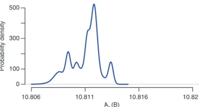
![Figure 1 shows an estimate of the probability density of the atomic weight of boron, produced by applica- applica-tion of a kernel density estimator [63], implemented in R funcapplica-tion density, to the sample of atomic weight values produced by Algorit](https://thumb-eu.123doks.com/thumbv2/123doknet/14051624.460226/20.892.78.425.749.937/estimate-probability-produced-estimator-implemented-funcapplica-produced-algorit.webp)
![Figure 2 shows that the materials, whose provenance is one of the commercial sources listed in Table 2, have atomic weights concentrated on the lower half of the interval [10.806, 10.821] that represents the standard atomic weight of boron](https://thumb-eu.123doks.com/thumbv2/123doknet/14051624.460226/21.892.157.816.124.341/figure-materials-provenance-commercial-concentrated-interval-represents-standard.webp)
![Fig. 7: Bivariate joint probability densities for the relative molecular masses of pairs of selected molecules depicted using hexagon bin smoothing [80]: the darker the shade of gray, the higher the density](https://thumb-eu.123doks.com/thumbv2/123doknet/14051624.460226/27.892.154.814.126.292/bivariate-probability-densities-relative-molecular-selected-molecules-smoothing.webp)
