HAL Id: hal-00299271
https://hal.archives-ouvertes.fr/hal-00299271
Submitted on 15 Mar 2006
HAL is a multi-disciplinary open access
archive for the deposit and dissemination of
sci-entific research documents, whether they are
pub-lished or not. The documents may come from
teaching and research institutions in France or
abroad, or from public or private research centers.
L’archive ouverte pluridisciplinaire HAL, est
destinée au dépôt et à la diffusion de documents
scientifiques de niveau recherche, publiés ou non,
émanant des établissements d’enseignement et de
recherche français ou étrangers, des laboratoires
publics ou privés.
A. H. Thieken, M. Müller, L. Kleist, I. Seifert, D. Borst, U. Werner
To cite this version:
A. H. Thieken, M. Müller, L. Kleist, I. Seifert, D. Borst, et al.. Regionalisation of asset values for
risk analyses. Natural Hazards and Earth System Science, Copernicus Publications on behalf of the
European Geosciences Union, 2006, 6 (2), pp.167-178. �hal-00299271�
© Author(s) 2006. This work is licensed under a Creative Commons License.
and Earth
System Sciences
Regionalisation of asset values for risk analyses
A. H. Thieken1, M. M ¨uller1,4, L. Kleist2,4, I. Seifert1,3, D. Borst3,4, and U. Werner3
1GeoForschungsZentrum Potsdam (GFZ), Section Engineering Hydrology and Data Center, Telegrafenberg, 14 473 Potsdam, Germany
2University of Karlsruhe (TH), Institute for Economic Policy Research, 76 128 Karlsruhe, Germany 3University of Karlsruhe (TH), Institute for Finance, Banking and Insurance, 76 128 Karlsruhe, Germany 4Center for Disaster Management and Risk Reduction Technology (CEDIM), 76 128 Karlsruhe, Germany
Received: 16 November 2005 – Revised: 19 January 2006 – Accepted: 19 January 2006 – Published: 15 March 2006
Abstract. In risk analysis there is a spatial mismatch of haz-ard data that are commonly modelled on an explicit raster level and exposure data that are often only available for ag-gregated units, e.g. communities. Dasymetric mapping tech-niques that use ancillary information to disaggregate data within a spatial unit help to bridge this gap. This pa-per presents dasymetric maps showing the population den-sity and a unit value of residential assets for whole Ger-many. A dasymetric mapping approach, which uses land cover data (CORINE Land Cover) as ancillary variable, was adapted and applied to regionalize aggregated census data that are provided for all communities in Germany. The re-sults were validated by two approaches. First, it was ascer-tained whether population data disaggregated at the commu-nity level can be used to estimate population in postcodes. Secondly, disaggregated population and asset data were used for a loss evaluation of two flood events that occurred in 1999 and 2002, respectively. It must be concluded that the algo-rithm tends to underestimate the population in urban areas and to overestimate population in other land cover classes. Nevertheless, flood loss evaluations demonstrate that the ap-proach is capable of providing realistic estimates of the num-ber of exposed people and assets. Thus, the maps are suf-ficient for applications in large-scale risk assessments such as the estimation of population and assets exposed to natural and man-made hazards.
1 Introduction
The project “Risk Map Germany” was launched by the Cen-ter of DisasCen-ter Management and Risk Reduction Technology (CEDIM) and is aimed at investigating and comparing losses
Correspondence to: A. H. Thieken
due to several types of natural hazards. To compare risks due to different natural and man-made disasters such as floods, windstorms and earthquakes a consistent conceptual frame-work of the risk analysis is needed. The frameframe-work chosen for the project “Risk Map Germany” is described in detail by Kleist et al. (2006)1. Here, only the basic ideas are given.
The term risk is used to describe the probability that a given loss will occur. Risk encompasses three aspects: hazard, vulnerability (susceptibility) and exposed assets or people. Whereas input data and methodologies for hazard and vulnerability assessments vary from hazard type to haz-ard type a uniform database of potentially exposed assets is essential for a consistent comparison of different risks (Gr¨unthal et al., 2006). Therefore, a working group was es-tablished with the aim of developing a spatially-distributed inventory of asset values for different economic sectors in whole Germany.
As a common risk indicator, by which quantitative esti-mates of different risks can be compared, direct economic losses to residential buildings were chosen. Thus, Kleist et al. (2006)1developed a method to estimate the asset value of residential buildings at the community level and delivered an inventory of assets for whole Germany. Like other exposure data such as population, these assets are, however, only avail-able at spatially aggregated areas, in this case communities. Chen et al. (2004) noticed that there is a spatial mismatch between hazard and exposure data: While hazard estimates are commonly modelled at a spatially explicit raster level, exposure data are often only available at spatially aggregated and coarse areal unit levels, e.g. community districts, census tracts or postcodes. Moreover, residential buildings and
pop-1Kleist, L., Thieken, A., K¨ohler, P., M¨uller, M., Seifert, I., Borst,
D., and Werner, U.: Estimation of the regional stock of residential buildings as a basis for comparative risk assessment for Germany, Nat. Hazards Earth Syst. Sci., submitted, 2006.
ulation are mainly concentrated in villages, cities and along roads so that a uniform distribution of exposure data within a community or postcode is not realistic. Therefore, asset val-ues should also be provided in a finer spatial resolution for loss modelling and risk analysis.
For the assessment of different types of natural hazards different resolutions of data are required. For example, Chen et al. (2004) showed that hailstorm risk assessments are more sensitive to the resolution of exposure data than earthquake risk assessments. For the risk assessment of insurance portfolios the requirements on data resolution of exposure data increase in the following order: windstorm, earthquake, flooding, man-made hazards (Munich Re, 2004). Whereas exposure data at the level of CRESTA (Catastro-phe Risk Evaluation and Standardizing Target Accumula-tion) zones is sufficient for windstorm and earthquake risk assessments, more accurate exposure data at the address or building level are required for flood risk assessment and particularly for the assessment of man-made hazards (Mu-nich Re, 2004). CRESTA-zones have become a widely ac-cepted standard in the international insurance industry (see http://www.cresta.org). In Germany, CRESTA-zones corre-spond to the level of five-digit postcodes (CRESTA, 2004).
A map with building specific assets cannot be provided on a nationwide scale as it is required for the project “Risk Map Germany”. In order to bridge the gap between aggre-gated census data and geocoded data, land use information is used to disaggregate census data. This type of mapping information is called dasymetric mapping and traces back to the work of Wright (1936). The aim of this paper is to adapt a dasymetric mapping algorithm for the disaggregation of population and asset values in Germany and to provide countrywide dasymetric maps of these variables. Before pre-senting the methods and results, a short overview of relevant literature on dasymetric mapping is given in the next section. Moreover, a validation of the method is performed within the context of risk analyses. Since flood risk assessments are rather sensitive to data resolution, the validation is done with a number of flood scenarios.
2 Literature review on dasymetric mapping
A dasymetric map depicts quantitative areal data using boundaries that divide the mapped area into zones of relative homogeneity with the purpose of best portraying the underly-ing statistical surface (Eicher and Brewer, 2001). Most dasy-metric mapping methods are mass-preserving, i.e. the total of the mapped variable in each origin zone is kept after dis-aggregation. Dasymetric zones are generated by using an-cillary information. According to MacEachren (1994), data representation via dasymetric mapping can be classified as a transition between smooth and stepped statistical surfaces.
In most of the investigations land cover data are used as ancillary data (e.g. Fisher and Langford, 1995; Yuan et al.,
1997; Martin et al., 2000; Eicher and Brewer, 2001; Mennis, 2003; Holt et al., 2004). An exception is the work of Chen et al. (2004), who used street buffers to roughly estimate in-habited areas in postcodes.
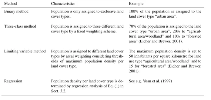
There are different methods of dasymetric mapping using land cover data (see Eicher and Brewer, 2001, for details and further references): the binary method, the three-class method, the limiting variable method and regression meth-ods. Table 1 provides an overview of the different mapping techniques.
With the binary method 100% of the census data are as-signed to exclusive land cover classes, such as urban areas or agricultural areas, whereas no data is assigned to other land cover classes like forest or water. The binary method is a specialized form of the limiting variable method (see below) and was originally developed by Langford et al. (1991) as a mapping technique.
For the three-class method a weighting scheme is used to assign population or other census data to three different land cover classes within each census district, e.g. urban, agri-cultural/woodland and forest. Other land cover classes like water receive no data. There are two major weaknesses of this method: the weights are subjectively determined and the method assumes a uniform distribution of land cover, i.e. it does not account for the actual area that is covered by each land cover class within a given census district (Eicher and Brewer, 2001; Mennis, 2003). Mennis (2003) proposes an algorithm that overcomes the second problem.
The limiting variable method was described by McCleary (1969). In this method, data is firstly assigned to all inhabit-able areas by simple areal weighting. In the next step, thresh-olds of maximum density that are derived from land use data or expert judgement, are set for particular land uses. These thresholds determine modifications of the data distribution: If a polygon density exceeds its threshold, the threshold den-sity is assigned to this polygon and the remaining data are distributed evenly among the remaining zones in the census district (Gerth, 1993, cited in Eicher and Brewer, 2001).
As a fourth type of method, multivariable regression is performed to examine the correlation between population counts from census and land cover types assuming that the total population of a census district is the sum of the prod-ucts of population densities and total areas of each land cover type in the district (e.g. Langford et al., 1991; Yuan et al., 1997). To ensure that the total population within a census district is preserved, a correction factor, i.e. the ratio of the total predicted population within one census district and the census data of that district, is used to adjust the estimates (Flowerdew and Green, 1989). Gallego (2001) developed a regression-like method that is based on data from two levels of aggregation and an iterative algorithm by which the coeffi-cients that describe the population density per land cover type are determined. Gallego (2001) further improved the method by distinguishing different types of communities (see below).
Table 1. Overview of dasymetric mapping techniques.
Method Characteristics Example Binary method Population is only assigned to exclusive land
cover types.
100% of the population is assigned to the land cover type “urban area”.
Three-class method Population is assigned to three different land cover type by a fixed weighting scheme.
70% of the population is assigned to the land cover type “urban area”, 20% to “agricul-tural area/woodland” and 10% to “forested area” (Eicher and Brewer, 2001).
Limiting variable method Population is assigned to different land cover types by areal weighting considering thresh-olds of maximum population density per land cover type.
The maximum population density is set to 50 inhabitants per square kilometre for land use type “agricultural area/woodland” and to 15 for “forested area” (Eicher and Brewer, 2001).
Regression Population density per land cover type is de-termined by regression analysis of Eq. (1) in Sect. 3.2.
See e.g. Yuan et al. (1997)
A number of studies deal with the comparison of different methods. However, Martin et al. (2000) emphasise that one of the key obstacles to the evaluation of dasymetric mapping techniques is the lack of definitive high resolution population data. Since the model performance is strongly influenced by the resolution and accuracy of the input data, input data quality is more important than algorithmic details (Martin et al., 2000).
In comparison to areal weighting and to different regres-sion methods the dasymetric binary method is the most accu-rate in the investigation of Fisher and Langford (1995). Bi-nary dasymetric mapping also outperforms an approach in which population is redistributed in proportion of a cell’s dis-tance to the centroids of the census districts (Martin et al., 2000). In the investigation of Eicher and Brewer (2001) the limiting variable method performs best in comparison to the binary as well as the three-class method. The most recently developed methods of Gallego (2001) and Mennis (2003) have not been compared so far.
Most of the studies focus on the distribution of popula-tion. Further research should be done to remodel other socio-economic variables and to assess the reliability of the results (Yuan et al., 1997). Therefore, the aim of this paper is to adapt the mapping approach of Gallego (2001) for the re-gionalisation of population and asset values in Germany and to provide countrywide dasymetric maps of these variables. Moreover, a validation of the method is performed using a number of flood scenarios.
3 Data and methods
3.1 Input data
For the application of the mapping approach of Gallego (2001) census data with boundaries of the census tracts as well as land use data are necessary. In the CEDIM project “Risk Map Germany” the following data sources have been used:
Census data were provided by INFAS Geodaten (2001). These data contain geometric information in boundary lines as well as census information about, e.g. population, house-holds or absolute and relative amount of different building types. The data are available in two spatial units which are defined by the administrative boundaries of the communities and the five-digit postcodes, respectively. Both topologies do not depend on each other and are thus partly incongruent. In general, the community level is used for the risk assessments in CEDIM and thus for the disaggregation of census data. The data on postcode level is used to validate the disaggre-gation of the population done on the community level.
Since the overall goal of this investigation is to perform a suitable dasymetric mapping approach to the estimates of as-sets for residential buildings per community given by Kleist et al. (2006)1, these data are also used as input.
CORINE (CoORdination of INformation on the Environ-ment) Land Cover data (CLC) for Germany – funded by the German Federal Environmental Agency and by the European Union – is used as ancillary dataset to perform dasymetric mapping. The CLC dataset gives a European wide overview of land use in 44 categories. The data evaluation is based on satellite imagery interpretation with a defined minimum
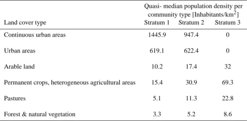
Table 2. Quasi-median population density Uc per land cover type and community type; Uc was determined by an iterative algorithm in Gallego (2001).
Quasi- median population density per community type [Inhabitants/km2] Land cover type Stratum 1 Stratum 2 Stratum 3 Continuous urban areas 1445.9 947.4 0
Urban areas 619.1 622.4 0
Arable land 10.2 17.4 32
Permanent crops, heterogeneous agricultural areas 15.4 30.9 69.3
Pastures 5.1 11.3 22.8
Forest & natural vegetation 3.3 5.2 8.6
size for different areas (25 ha), so CLC areas show a high de-gree of generalization. The used dataset reflects the land use pattern in the year 2000 (Mohaupt-Jahr and Keil, 2004).
3.2 Method for regionalisation of aggregated data – dasy-metric mapping
Gallego (2001) developed a model for the distribution of cen-sus population on the basis of the CLC dataset for whole Eu-rope. It is based on the approach that the population in a community m can be described as the sum of the areas of different land cover classes in that community multiplied by a respective population density:
Xm= X c ScmYcm (1) Ycm=UcWm (2) Xm : population in community m
Scm: area of land cover class c in community m
Ycm: population density of land cover class c in
community m
Uc : quasi-median population density of land cover class
c ( determined by an iterative algorithm) Wm: correction factor for community m
The population density consists of a quasi-median popula-tion density and a correcpopula-tion factor. The correcpopula-tion factor Wm ensures that the total population of a community will
be correctly estimated by this approach, and is calculated by the ratio of the census data of that community and the total predicted population within one community using the coeffi-cients Ucin Table 2. The coefficients Ucare given in Gallego
(2001) distinguishing six land cover classes and three types of communities (Table 2). The land cover classes are derived by aggregating the original 44 CLC classes into the follow-ing categories: 1) continuous urban areas, 2) urban areas
(in-cluding industrial, commercial, and transport units as well as artificial non-agricultural vegetated areas for recreational purposes), 3) arable land, 4) permanent crops and heteroge-neous agricultural areas, 5) pastures, 6) forests and areas cov-ered by natural vegetation. All other land cover types such as water, wetlands, open spaces with little or no vegetation as well as mine, dump and construction sites are classified as uninhabitable.
Three types (strata) of communities are derived by com-paring the population density of a community with the pop-ulation density at the corresponding regional level. For this purpose the EU Nomenclature of Territorial Units for Statis-tics (NUTS) is used. NUTS is a hierarchical classification, that subdivides each EU Member State into a number of NUTS1 regions, each of which is in turn subdivided into a number of NUTS2 regions etc. In Germany, the NUTS1 level refers to the federal states (Bundesl¨ander), the NUTS2 level to regions and the NUTS5 level to communities (Eurostat, 2005).
Gallego (2001) defines three types of communities: The first stratum consists of communities (NUTS5) with an over-all population density that is twice as high as the population density of the corresponding NUTS2 region or even higher. In contrast to Gallego (2001), communities with more than 50 000 inhabitants are generally assessed as densely popu-lated and are thus assigned to stratum 1 in this study.
The second stratum includes communities (NUTS5) with an overall population density that is lower than the twofold population density of the corresponding NUTS2 region. In addition, urban areas (i.e. land cover classes 1 or 2) must be present in the community.
The third stratum contains communities (NUTS5) with an overall population density that is lower than the twofold pop-ulation density of the corresponding NUTS2 region and the
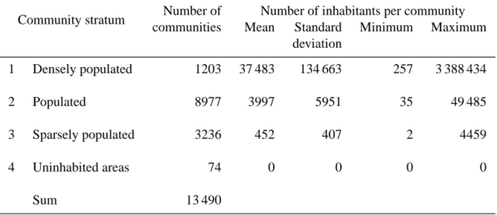
Table 3. Number of communities and inhabitants per community stratum in Germany. In stratum 4 large uninhabited areas that are modelled
as independent polygons in the INFAS geo-dataset are summarised.
Community stratum Number of Number of inhabitants per community communities Mean Standard Minimum Maximum
deviation 1 Densely populated 1203 37 483 134 663 257 3 388 434 2 Populated 8977 3997 5951 35 49 485 3 Sparsely populated 3236 452 407 2 4459 4 Uninhabited areas 74 0 0 0 0 Sum 13 490
community area shows NO urban areas in the CLC dataset (i.e. no areas of the land cover classes 1 or 2).
In this study, a fourth stratum is introduced for large un-inhabited areas that do not belong to any community in Ger-many and are modelled as independent polygons in the IN-FAS geo-dataset. Such areas can be found in mountainous regions (cf. Fig. 3a). In this stratum all coefficients Uc are
zero.
The number of communities in each stratum and the pop-ulation statistics in Germany are summarized in Table 3.
After reclassifying the original CLC dataset into the six land cover classes and after determining the stratum of each community, a correction factor Wm is calculated for each
community within the GIS ArcView by the following equa-tion: Wm= XmINFAS P c ScmUc (3)
Wm : correction factor for community m
XmINFAS: population in community m according to INFAS Geodaten (2001)
Scm : area of land cover class c in community m
Uc : quasi-median population density of land cover
class c (determined by an iterative algorithm) For the regionalisation of population data, the community boundaries are first intersected with the boundaries of the re-classified CLC dataset. The population densities Ucand the
correction factors Wmare then assigned to each land cover
class and community, respectively. The population density of a land cover polygon is determined by Eq. (2). The total population within a polygon is estimated by multiplying the Ycmwith the respective polygon area.
A regionalisation of the asset values of residential build-ings provided by Kleist et al. (2006)1is performed by multi-plying the estimated population of a polygon with the per-capita asset of residential buildings of the corresponding
community. For the purpose of risk analysis a map represent-ing unit values for residential buildrepresent-ings in Euro per square meter is more useful. Therefore the asset value per polygon is divided by the polygon area. The mapping procedure is outlined in Fig. 1.
3.3 Model validation
The adapted method of Gallego (2001), i.e. the regionalisa-tion of popularegionalisa-tion and assets, is validated by two approaches. In a first attempt, the disaggregated map of population den-sity is used to estimate the total population in five-digit postcodes. The “real” population per postcode is also pro-vided by INFAS Geodaten (2001). As mentioned above, the topologies of community boundaries and postcodes are in-dependent from each other. The error of the population per postcode is mapped and analyzed statistically.
In a second approach the regionalisation method is val-idated by intersecting the disaggregated population density map and the dasymetric map of the unit residential values with flood lines of real flood events. By means of intersec-tion, the number of affected people and the amount of af-fected residential assets can be estimated. A rough loss esti-mation is performed, as well. These estimates are then com-pared with figures given by the authorities. This procedure is also performed for the aggregated data on community level in order to analyse whether better results are achieved with disaggregated data.
Since the data used for the estimation and regionalization of residential values refers to the year 2000, flood scenarios around this reference year are chosen for validation. Two flood events took place along the river Danube in 1999 and along the rivers Elbe and Danube in 2002, respectively. The inundation areas were provided by several German environ-mental and cartographic agencies and are shown in Fig. 2.
To estimate the assets at risk due to these flood events, the values of Kleist et al. (2006)1 have to be adjusted by
con-JOIN Land use area within community borders
JOIN
Population density for each land use area in a community
Population per land use area
Unit value of residential buildings in Euro per sqm Value of residential buildings in a land use area
CALC \
Community Borders (INFAS) Land use data (CORINE)
JOIN
Replacement costs per capita and community (INFAS) Revised population density per land use type and community (Gallego, 2001)
CALC *
Fig. 1. Map model for regionalisation of asset values (dasymetric mapping).
Table 4. Areas of land cover types according to reclassified CORINE Land Cover data in Germany and estimated population per land cover
type following the model of Gallego (2001).
Land cover type Area [km2] % Area Estimated population % Estimated population Continuous urban areas 231.7 0.1% 1 919 083 2.3% Urban areas 27 412.8 7.7% 69 082 677 83.8% Arable land 136 825.0 38.3% 5 963 433 7.2% Permanent crops, heterogeneous agricultural areas 23 127.3 6.5% 2 231 911 2.7%
Pastures 54 052.8 15.1% 1 706 884 2.1%
Forest & natural vegetation 109 025.0 30.5% 1 536 091 1.9%
Uninhabited areas 6604.7 1.8% 0 0.0%
Sum 357 279.3 100.0% 82 440 079 100.0%
Total population according to INFAS 82 440 309
Absolute error −230
Relative error −0.0003%
struction indices of the year of the flood. Construction in-dices are published by the Federal Statistical Agency (Statis-tisches Bundesamt, 2004). For the years 1999 and 2002, the original assets have to be corrected by a factor of 0.997 and 0.999, respectively.
4 Results and discussion
4.1 Population density
The general composition of the aggregated land cover classes in Germany on the basis of the CLC dataset and the total
amount of population which is assigned to each land cover class by the adapted algorithm of Gallego (2001) are sum-marized in Table 4. Due to the introduction of the correction factors Wm the total population is estimated correctly (see
Eq. 3).
Urban areas cover less than 8% of the whole area in Ger-many, but more than 80% of the population are assigned to this land cover class. In contrast, arable land and forest cover more than 30% of the area each, but only 7% and 2% of the population are assigned to these classes, respectively (Ta-ble 4). These results are consistent with those of Gallego (2001).
Catchment areas Rhine Elbe/Labe Danube Weser Ems Oder/Odra Inundated Area 100 0 100 km
A:
B:
Fig. 2. Flooded areas in Germany during the Whitsun flood in May 1999 (A) and during the flood of August 2002 (B). (Data sources:
ATKIS®DLM1000, VG250, Flood lines of the Elbe flood on the basis of satellite picture © Federal Agency of Cartography and Geodesy 2003; Flood plain of the Mulde river, UFZ Leipzig 2003; Inundated areas in Saxony during the flood 2002: Saxonian Agency of Environment and Geology, Water resources management information system of the Bavarian water resources management office, 2004, http://www.bayern. de/lfw).
Figure 3 shows the spatial distribution of population den-sity in Germany as well as the differences between a choro-plethic (Fig. 3a) and a dasymetric (Fig. 3b) mapping ap-proach. It is obvious that a high population density exists around the big cities e.g. Hamburg, Berlin, the Ruhr area (around the cities of Dortmund, Essen, and Duisburg), K¨oln (Cologne), Frankfurt, Stuttgart and M¨unchen (Munich). In comparison to the choroplethic map in Fig. 3a, settlement patterns and agglomeration areas are highlighted in more de-tail by the dasymetric mapping approach in Fig. 3b.
4.2 Distribution of assets
On the basis of the population distribution shown in Fig. 3b the asset values of Kleist et al. (2006)1are distributed by mul-tiplying the per-capita asset value for residential buildings of a community with the number of inhabitants per polygon of the dasymetric map in that community shown in Fig. 3b. To better compare the results, the total asset values are trans-formed into unit values per square meter. The results are shown in Fig. 4a as a choroplethic map per community and in Fig. 4b per polygon of the dasymetric map. Due to the al-gorithm, the spatial pattern of the asset distribution correlates well with the pattern of the population density presented in
Fig. 3b. Again, the dasymetric mapping approach imparts a more detailed picture of the asset distribution.
4.3 Model validation and application
As outlined above, the validation of the model is performed by two approaches: firstly, by estimating population in post-codes and secondly, by using the maps for flood loss evalua-tions.
In Fig. 5 the percentage of error in estimating population in postcodes is shown. The error is defined as the difference between the population per postcode given by INFAS Geo-daten (2001) and the population per postcode estimated from the disaggregated population shown in Fig. 3b. Thus, posi-tive (red) error values in Fig. 5 indicate an underestimation of the “real” population given by INFAS, whereas negative (blue) values indicate an overestimation of the “real” popu-lation. The mean error amounts to −3%, i.e. on average the population in postcodes is slightly overestimated if the esti-mate is derived from the dasymetric population map shown in Fig. 3b. The overestimation is due to the fact that the area of the postcodes was not considered in this calculation. If an area-weighted mean is calculated, the mean estimation error
Table 5. Average composition of land cover classes in postcodes with different population estimation errors.
Land cover type Postcodes with a Postcodes with a Postcodes with a All post-codes population estimation population estimation population estimation
error of <−50% error of >50% error of ±10% (underestimation) (overestimation)
Continuous urban areas 8% 3% 0% 1%
Urban areas 78% 45% 10% 18%
Arable land 4% 22% 34% 31%
Permanent crops, heterogeneous 1% 3% 9% 8% agricultural areas
Pastures 2% 7% 15% 14%
Forest & natural vegetation 3% 16% 29% 26%
Uninhabited areas 3% 4% 2% 2% Number of postcodes 169 282 6559 8257 100 km 0 100
B:
A:
# # # # # # # # # # # ## # # # # # # # # # # # # Potsdam Köln Bonn Kiel Essen Mainz Bremen Erfurt München Leipzig Hamburg Rostock Dresden Duisburg Dortmund Hannover Schwerin Karlsruhe Stuttgart Wiesbaden Magdeburg Flensburg Saarbrücken Frankfurt a.M. Berlin # # # # # # # # # # # # # # # # # # # # # # # # # Köln Bonn Kiel Essen Mainz Bremen Erfurt München Leipzig Hamburg Rostock Dresden Duisburg Dortmund Hannover Schwerin Karlsruhe Stuttgart Wiesbaden Magdeburg Flensburg Saarbrücken Frankfurt a.M. Potsdam Berlin Population density [Inhabitants/km²] 0 > 0 - 100 > 100 - 500 > 500 - 1000 > 1000 - 5000 > 5000 - 10000 > 10000Fig. 3. (A): Choroplethic map of population density based on INFAS Geodaten (2001) per community. (B): Dasymetric map of population
density based on INFAS Geodaten (2001), CORINE Land Cover 2000 and the adapted mapping algorithm of Gallego (2001). Data are given in number of inhabitants per square kilometre.
amounts to −0.0003% that was also indicated as estimation error in Table 4.
It is obvious that large errors particularly occur in the re-gions of the big German cities (Fig. 5). This can be explained by two aspects. At first, the postcodes in the big cities are much smaller than the corresponding community area. For example, the community/city of Berlin is divided into 190
postcodes, Hamburg into 101, M¨unchen (Munich) into 74, D¨usseldorf into 38, and Essen into 32. On the other hand, several rural communities are often summarized into one postcode, e.g. the largest postcode “Templin” covers 20 com-munities. Altogether, for the 13 490 communities in Ger-many only 8257 postcodes exist. Therefore, the validation process has different conditions for rural and urban areas.
100 km 0 100
B:
A:
# # # # # # # # # # # ## # # # # # # # # # # # # Potsdam Köln Bonn Kiel Essen Mainz Bremen Erfurt München Leipzig Hamburg Rostock Dresden Duisburg Dortmund Hannover Schwerin Karlsruhe Stuttgart Wiesbaden Magdeburg Flensburg Saarbrücken Frankfurt a.M. Berlin # # # # # # # # # # # ## # # # # # # # # # # # # Köln Bonn Kiel Essen Mainz Bremen Erfurt München Leipzig Hamburg Rostock Dresden Duisburg Dortmund Hannover Schwerin Karlsruhe Stuttgart Wiesbaden Magdeburg Flensburg Saarbrücken Frankfurt a.M. Potsdam Berlin Unit Value of Residential Buildings [Euro/m²] 0 > 0 - 50 > 50 - 100 > 100 - 250 > 250 - 500 > 500Fig. 4. (A): Choroplethic map of assets of residential buildings according to Kleist et al. (2006)1per community. (B): Dasymetric map of assets of residential buildings based on INFAS Geodaten (2001), CORINE Land Cover 2000, the adapted mapping algorithm of Gallego (2001) and the per-capita values calculated by Kleist et al. (2006)1. Data are given in asset value of residential buildings per square meter.
Whereas the population of postcodes in rural areas tends to be summarized from several communities, the population of postcodes in urban areas has to be estimated from a frac-tion of the corresponding community. Thus, in urban areas a higher accuracy of the disaggregated data is requested.
The land use composition is a second aspect that is im-portant for this topic. For all postcodes with low or high estimation errors the mean composition of the seven aggre-gated land cover classes is shown in Table 5. In postcodes with a low population estimation error of up to ±10%, the composition of the land cover classes corresponds approx-imately to the average composition of all postcodes except for urban areas. In contrast, the postcodes with a high un-derestimation, i.e. with a population estimation error of less than −50%, are characterized by a very high percentage of urban areas. Other land cover classes are clearly underrepre-sented (Table 4). That means that densely populated areas in the city centres are not correctly modelled by the adapted ap-proach of Gallego (2001). Figure 5 illustrates that postcodes with high underestimations are often adjacent to areas with high overestimations. Table 5 shows that postcodes with a high overestimation, i.e. with a population estimation error of more than 50%, still contain a share of urban areas above average. However, there is also a considerable amount of arable and forested land. Altogether, it must be concluded
that the algorithm tends to underestimate the population in urban areas and to overestimate other land cover classes.
In the second validation procedure two flood events that occurred in May 1999 (Fig. 2a) and August 2002 (Fig. 2b), respectively, are analyzed. Both aggregated census data and data disaggregated by dasymetric mapping were used to es-timate the number of exposed people and residential assets. The results are summarized in Table 6. The values provided by the authorities are given in Table 7.
The number of affected people can only be compared for the Pentecost flood 1999 in Bavaria. Surprisingly, the num-ber of affected people given by the authorities is better es-timated on the basis of aggregated data. However, also the estimate with disaggregated data is in a similar order of mag-nitude (Tables 6 and 7).
With regard to the residential assets, the values in Tables 6 and 7 cannot be compared directly, since in Table 7 the losses that occurred to residential buildings are given, whereas in Table 6 the total sum of exposed assets is calculated. There-fore, an overall loss ratio of 12.3% which was the mean loss ratio among more than 1000 residential buildings during the August 2002 flood in a survey of Thieken et al. (2005) was assumed to roughly estimate the damage to residential build-ings (Table 6). Although it was not expected that the losses in all affected areas would be modelled correctly with a
uni-# # # # # # # # # # # ## # # # # # # # # # # # # Potsdam Köln Bonn Kiel Essen Mainz Bremen Erfurt München Leipzig Hamburg Rostock Dresden Duisburg Dortmund Hannover Schwerin Karlsruhe Stuttgart Wiesbaden Magdeburg Flensburg Saarbrücken Frankfurt a.M. Berlin
Population Estimation Error [%] < -50 > -50 - -25 > -25 - -10 > -10 - 10 > 10 - 25 > 25 - 50 > 50 No Data 100 0 100 km
Fig. 5. Relative population estimation error in per cent per postcode. The error is defined as: error = (population per postcode as given by
INFAS Geodaten (2001)) – (population per postcode as estimated on the basis of Fig. 3b); blue: overestimation of the INFAS-population; red: underestimation of the INFAS-population.
Table 6. Estimates of the number of exposed people and residential assets for two flood events in Germany as well as rough estimates of the
losses to residential buildings (put in parentheses) assuming an average loss ratio of 12.3% according to the work of Thieken et al. (2005).
Flood Event Federal State Estimated number of affected people Estimated sum of exposed assets of residential buildings (and estimated loss) in the year of the flood [million ] Aggregated data Disaggregated data Aggregated data Disaggregated data August 2002 Saxony 159 212 212 155 7490 (921) 9926 (1221) Saxony-Anhalt 129 655 54 743 5354 (658) 2268 (279)
Bavaria 9106 11 149 494 (61) 619 (76)
May 1999 Bavaria 106 329 69 444 5507 (677) 3624 (446)
form loss ratio, this simple approach was chosen to compare the feasibility of aggregated and disaggregated data.
With this simple loss estimation, the magnitude of losses to residential buildings in the three most affected federal states Saxony, Saxony-Anhalt and Bavaria is surprisingly well estimated for the August 2002 flood if disaggregated data are used (compare Table 6 and Table 7). The use of ag-gregated data leads to a clearer underestimation of losses for Saxony and a clearer overestimation for Saxony-Anhalt than the use of disaggregated data. Both methods tend to overes-timate the losses in Bavaria. This might be due to the fact that the 2002 flood event was less severe in Bavaria. Thus, a mean loss ratio of 12.3% is probably too high for this
re-gion. On the contrary, the value might be too low for Saxony, the most affected state during the August 2002 flood. Thus, a more sophisticated loss estimation model should improve the results.
The good results for the August 2002 flood cannot be re-produced for the flood in 1999. Both methods lead to an enormous overestimation of loss (compare Table 6 and Ta-ble 7). Also in this example, however, the results with ag-gregated data are inferior to those with disagag-gregated data. In contrast, the number of affected people is estimated quite well (see above). Altogether, this flood event needs further investigation.
Table 7. Number of affected people, total damage and damage to residential buildings during two flood events in Germany as quoted by the
authorities (Sources: Deutsche R¨uck, 2000; IKSE, 2004; SSK, 2004).
Flood Event Affected Federal State Number of affected people Total damage Damage to residential buildings August 2002 Saxony No data 8700 million 1706 million
Saxony-Anhalt No data 1187 million 246 million * Bavaria No data 198 million No data May 1999 Bavaria 100 000 393 million 98 million * data include damage to household contents
Considering the fact that the loss estimation was done with a very simple assumption, the results show that the approach is capable of estimating a realistic number of exposed peo-ple and residential assets. In most of the cases, the use of disaggregated data provides better results than the use of ag-gregated data. For a thorough validation, however, better loss estimation models have to be applied and further flood events have to be analyzed.
5 Conclusions
In order to provide exposure data that meet the demands of large-scale risk assessments a dasymetric mapping approach was successfully performed. The approach of Gallego (2001) is based on a regression-like model that uses CORINE land cover data as ancillary variable to distribute census popula-tion. In this study, the model was adapted to also map asset values of residential buildings and was then applied to all of Germany. As a result maps showing the population density and a unit value of residential assets can be presented for whole Germany. These maps can be used as input data for the estimation of population and assets at risk. The results were validated in two ways.
From the validation it has to be concluded that the algo-rithm tends to underestimate the population in urban areas and to overestimate population in other land cover classes. Therefore, high errors might occur, especially in urban ar-eas. Nevertheless, good results were achieved when estimat-ing people and assets exposed to the August 2002 flood that hit large parts of Germany. Such satisfying results could not be reproduced for a flood that occurred in 1999 in South-ern Germany. All things considered, however, this approach does yield realistic estimates of exposed people and vulnera-ble assets.
For a thorough validation further flood events and scenar-ios of other natural disasters, e.g. windstorms or earthquakes, should be analyzed. Future analyses should include more so-phisticated loss models. Besides, upcoming research may lead in two other directions: First, the method used here should be evaluated in comparison to other dasymetric map-ping methods. As a second direction of research, further pos-sible applications of the presented maps should be
investi-gated. In case of a disaster there is a need for quick and reli-able loss estimates in order to provide enough resources for loss compensation and recovery. The presented maps could serve as an input to such a system. Research on this topic would be important for the general improvement of current disaster management.
Acknowledgements. The work is part of the project “Risk Map
Germany” of the Center for Disaster Management and Risk Reduc-tion Technology urlhttp//:www.cedim.de, a joint venture between the GeoForschungsZentrum Potsdam (GFZ) and the University of Karlsruhe (TH). We thank the GFZ Potsdam and the TH Karlsruhe for financial support.
Edited by: H. Kreibich Reviewed by: three referees
References
Chen, K., McAneney, J., Blong, R., Leigh, R., Hunter, L., and Mag-ill, C.: Defining area at risk and its effect in catastrophe loss es-timation: a dasymetric mapping approach, Appl. Geography, 24, 97–117, 2004.
CRESTA: Accumulation Assessment Zones Earth-quake/Windstorm/Flood in Germany, CRESTA 11, 2004, retrieved at http://www.cresta.org on 10 November 2005. Deutsche R¨uck: Das Pfingsthochwasser im Mai 1999, Deutsche
R¨uckversicherungsgesellschaft, D¨usseldorf, 2000.
Eicher, C. L. and Brewer C. A: Dasymetric Mapping and Areal Interpolation: Implementation and Evaluation, Cartography and Geographic Information Science, 28(2), 125–138, 2001. Eurostat: http://europa.eu.int/comm/eurostat/ramon/nuts/basicnuts
regions en.html, 2005.
Fisher, P. F. and Langford, M.: Modelling the errors in areal in-terpolation between zonal systems by Monte Carlo simulation, Environment and Planning A, 27, 211–224, 1995.
Flowerdew, R. and Green, M.: Statistical methods for inference between imcomparable zonal systems, in: Accuracy of spatial databases, edited by: Goodchild, M. and Gopal, S., New York, Taylor and Francis, 239–248, 1989.
Gallego, J.: Using land cover information to map population den-sity, Statistical Commission and Economic Commission for Eu-rope, Conference of European Statisticians, Tallinn, Estonia, Working Paper No. 21, 1–10, 2001.
Gr¨unthal, G., Thieken, A. H., Schwarz, J., Radtke, K. S., Smolka, A., and Merz, B.: Comparative risk assessment for the city of Cologne, Germany – storms, floods, earthquakes, Nat. Hazards, 38(1–2), 21–44, doi:10.1007/s11069-005-8598-0, 2006. Holt, J. B., Lo, C. P., and Hodler, T. W.: Dasymetric estimation of
population density and areal interpolation of census data, Car-tography and Geographic Information Science, 31(2), 103–121, 2004.
IKSE (International Commission for the Protection of the Elbe): Dokumentation des Hochwassers vom August 2002 im Einzugs-gebiet der Elbe (Documentation of the flood in August 2002 in the Elbe catchment) (in German), Magdeburg, 2004.
INFAS GEOdaten: Das DataWherehouse, Bonn, INFAS GEOdaten GmbH, Status: December 2001.
Langford, M., Maguire, D. J., and Unwin, D. J.: The areal interpo-lation problem: estimating popuinterpo-lation using remote sensing in a GIS framework, in: Handling geographical information, edited by: Masser, I. and Blakemore, M., London, Longman, 55–77, 1991.
MacEachren, A. M.: Some truth with maps: A Primer on sym-bolization and design, Washington, Assoc. Amer. Geographers, 1994.
Martin, D., Tate, N. J., and Langford, M.: Refining population sur-face models: Experiments with Northern Ireland census data, Transactions in GIS, 4(4), 343–360, 2000.
McCleary, G. F.: Cartography, geography, and the dasymetric method, PhD Thesis, University of Wisconsin, 1969.
Mennis, J.: Generating surface models of population using dasy-metric mapping, Professional Geographer, 55(1), 31–42, 2003. Mohaupt-Jahr, B. and Keil, M.: The CLC 2000 project in Germany
and environmental applications of land use information. Work-shop: CORINE Land Cover 2000 in Germany and Europe and its use for Environmental Applications, edited by: Federal Envi-ronmental Agency (Umweltbundesamt), Berlin, 20–21 January, 37–45, 2004.
Munich Re: Geographical Underwriting, TOPICS geo: Jahresr¨uckblick Naturkatastrophen 2003, 44–49, 2004.
SSK (S¨achsische Staatskanzlei – Saxonian State Chancellery): Der Stand des Wiederaufbaus, 3 pp., Materialien zur Kabinetts-Pressekonferenz am 3. Februar 2004 (in German), Dresden, Press release 3 February 2004.
Statistisches Bundesamt (Federal Statistical Agency): Baupreisin-dizes November 2003, Statistisches Bundesamt, Fachserie 17, Reihe 4, Wiesbaden, 2004.
Thieken, A. H., M¨uller, M., Kreibich, H., and Merz, B.: Flood damage and influencing factors: New insights from the August 2002 flood in Germany, Water Resour. Res., 41(12), W12430, doi:101029/2005WR004177, 2005.
Wright, J. K.: A method of mapping densities of population with Cape Cod as an example, Geographical Review, 26, 103–110, 1936.
Yuan, Y., Smith, R. M., and Limp, W. F.: Remodeling census popu-lation with spatial information from Landsat TM Imagery, Com-put., Environ. Urban Syst., 21(3–4), 245–258, 1997.