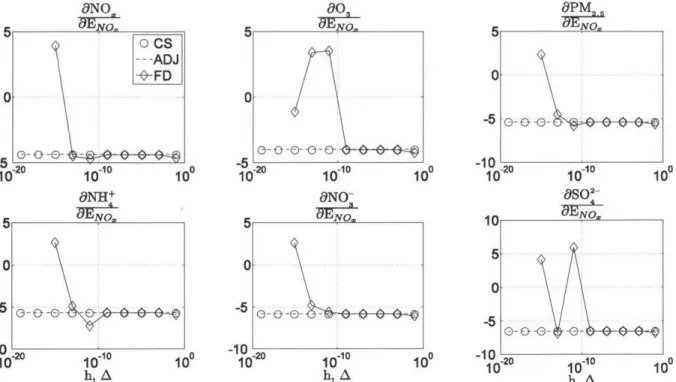
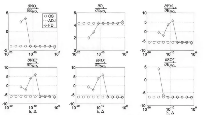
Application of the complex step method to chemistry-transport modeling
Texte intégral
Figure
Documents relatifs
If user fees are set as to allow some degree of free riding, an increase in enforcement in j can increase the demand of region i’s spillover good.. The sign of the former effect
Un panel limité de cités complète l’éventail précédent : une ville à fonction touristique forte et à image prestigieuse (Cannes, et 16 réunions
Dans un contexte où la sélection assistée par marqueurs n’a jamais pu trouver sa place pour d’autres caractères que la résistance aux ravageurs, la sélection génomique offre
This chapter presents a baseline local search strategy which is a receding horizon opti- mization over a dynamic probability map. A global search strategy is developed
Teneurs en chlore (Cl TOT , Cl OE1 et Cl ONE ) obtenues par analyseur d’AOX pour les échantillons VF2014 irradiés après 54 jours d’incubation en condition anaérobie ré-inoculés
Page 77 Figure 53 – Evolution du retrait en fonction du temps pour le BFUP A ayant subi un traitement thermique de premier type (réalisé à température modérée). Page 78 Figure 54
Bilan d'eau en trois points de la nappe phréatique générale du Tchad Water balance in three points of the water table aquifer of Chad.. Jean-Louis SCHNEIDER (1) et Dominique THIERY
In the following, we will show that a reduction of the intensity light-shift a can also be achieved by adjusting the temperature of the MEMS cell (instead of the modulation
