Application of robust and inverse optimization in transportation

Application of Robust and Inverse Optimization in

S

nMASSACHUSETTS

Tr-ansportation

by

SEPO

2 2010

Thai Dung Nguyen

_LIBRARIES

B.E. Electrical Engineering, National University of Singapore, 2009

Submitted to the School of Engineering

ARCHIVES

in partial fulfillment of the requirements for the degree of

Master of Science in Computation for Design and Optimization

at the

MASSACHUSETTS INSTITUTE OF TECHNOLOGY

September 2010

Massachusetts Institute of Technology 2010.

A uthor ...

Certified by...

All rights reserved.

. . . . . . . . . . . . . . . . . . . . . . . . . . . . . . .

chool of Engineering

August 4, 2010

mitris J. Bertsimas

Boeing Professor of Operations Research

Theris Supervisor

Certified by....

...

.

Georgia Perakis

William F. Pounds Professor of Operations Research

Thesis Supervisor

Accepted by...

C.-Karen Willcox

Associate Professor of Aeronautics and Astronautics

Codirector, Computation for Design and Optimization Program

Application of Robust and Inverse Optimization in

Transportation

by

Thai Dung Nguyen

Submitted to the School of Engineering on August 4, 2010, in partial fulfillment of the

requirements for the degree of

Master of Science in Computation for Design and Optimization

Abstract

We study the use of inverse and robust optimization to address two problems in transportation: finding the travel times and designing a transportation network. We assume that users choose the route selfishly and the flow will eventually reach an equilibrium state (User Equilibrium).

The first part of the thesis demonstrates how inverse and robust optimization can be used to find the actual travel times given a stable flow on the network and some noisy information on travel times from different users. We model the users' perception of travel times using three different sets and solve the robust inverse problem for all of them. We also extend the idea to find parametric functional forms for travel times given historical data. Our numerical results illustrate the significant improvement obtained by our models over a simple fitting model.

The second part of the thesis considers the network design problem under de-mand uncertainty. We show that for affine travel time functions, the deterministic problem can be formulated as a mixed integer programming problem with quadratic objective and linear constraints. For the robust network design problem, we propose a decomposition scheme: breaking a tri-level programming problem into two smaller problems and re-iterating until a good solution is obtained. To deal with the ex-pensive computation required by large networks, we also propose a heuristic robust simulated annealing approach. The heuristic algorithm is computationally tractable and provides some encouragingly results in our simulations.

Thesis Supervisor: Dimitris J. Bertsimas Title: Boeing Professor of Operations Research Thesis Supervisor: Georgia Perakis

Acknowledgments

I would like to express my heartfelt gratitude to all the people who have helped make this project an enjoyable and fruitful experience.

First and foremost, I would like to thank my advisors, Prof. Dimitris Bertsimas and Prof. Georgia Perakis, for their expert guidance. It is my great honor to have an opportunity to work with two of the best professors in Operations Research today.

I would like to thank Dimitris for his mentorship. His creative ideas and insightful comments have always guided my research. Moreover, his enthusiasm, belief, and optimism has taught me a great lesson in life. Since my first day as his student, Dimitris has been always asking me to be self-confident. Living in a top intellectual environment in the world, this was not easy at first. However, I have come to realize that self-reliance and a positive attitude will help me to mature and to succeed in life.

I am deeply grateful to Georgia for her expertise, kindness and patience. Despite

her busy schedule, she always spares time for me to present my ideas. She also explains things very carefully and makes sure that I fully understand her. Her invaluable knowledge in the area of variational inequalities and network equilibrium always helps me to enhance the horizon of my research and encourages me to explore new ideas and topics.

I would like to thank SMA program for creating such a wonderful opportunity.

The SMA scholarship brings me to one of the places I have ever dreamed of. I would to thank Laura Koller for her sincere help in the CDO program.

In addtion, I feel very lucky to have many wonderful friends here, who have enriched my life and made it more enjoyable than I could ever expected. I would like to thank Kil Dong Kwak. Not only being a great friend, his persistence has taught me a lot. I will remember my discussions with Henry Chen and my other classmates. Besides, I do really enjoy my soccer games with my Redlobster gang and tennis games with Mr. Venu. I am also very grateful to my friends, who are not here, for their constant support and encouragement.

Last but not least, I am immensely indebted to my family for their unconditional love, encouragement and care. You are always the unlimited source of power for me to overcome any obstacles. I would not be able to come all my way today, without your strong support. I owe you more than I could express.

Contents

1 Introduction 13

1.1 Uncertainty in Transportation Problems... .. 13

1.2 Contribution of the thesis... . . . .. 14

1.3 Structure of the thesis . . . . 15

1.4 Notations. . ... .. 16

2 Review of Robust Optimization 19 2.1 Robust Linear Optimization . . . . 19

2.2 Robust Simulated Annealing . . . . 21

3 User Equilibrium, VI and Optimization Formulations 23 3.1 User Equilibrium . . . . 23

3.2 VI and optimization formulation . . . . 24

4 The Inverse Optimization Problem to Find Travel Times 27 4.1 Introduction ... . . . . . . . . 27

4.2 Formulation... . . . . . . 28

4.3 Algorithms... . . . . . . . . 30

4.4 Computational Results . . . . 42

4.5 C onclusions . . . . 51

5 A Network Design Problem under User Equilibrium and Demand Uncertainty 53 5.1 Introduction... . . . . . . . . . .. 53

5.2 Deterministic Network Design Problem . . . . 56

5.3 Robust Network Design Problem . . . . 58

5.4 Computational Results.. . . . . . . . 63

5.4.1 Deterministic Network Desgin problem . . . . 63

5.4.2 Robust Network Design Problem . . . . 70

5.5 C onclusions . . . . 72

List of Figures

4-1 Deterministic solution. Total error = 20. . . . . 42

4-2 Robust solution (a) for Set E1 and box plot (b) for 1000 cases . . . . 43

4-3 Robust solution for Set E2 when B = 50. Total error = 20. . . . . 44

4-4 Robust solution (a) for Set E3 and box plot (b) for 1000 cases when B = 140 . . . . 44

4-5 Worst case error (a) and nominal case error (b) with varying uncer-tainty budget . . . . 45

4-6 Number of iteration with varying budget B . . . . 45

4-7 Parameter a when L = 20%. ... . . . . . ... 46

4-8 Parameter b when L = 20% . . . . 47

4-9 Fitting total squared error with varying uncertainty level(%) . . . . . 47

4-10 Fitting total squared error with varying p(L = 5%)... . . ... 48

4-11 Fitting parameter a when L=10% . . . . 48

4-12 Fitting parameter b when L=10% . . . . 49

4-13 Total squared error with varying uncertainty level L (%) . . . . 49

4-14 Total Fitting Error with varying uncertainty level . . . . 50

5-1 N etw ork 1 . . . . 63

5-2 Sioux Falls network . . . . 65

5-3 Total Cost and computation time (sec) with different M. Total Budget B=20.. ... .. .. .. .. ... .. .. .. .. .. ... ... 65

5-4 Total Cost and computation time (sec) with total Budget B = 24 . . 66

5-6 Total travel time with varying M . . . . 68

5-7 Computation time (sec) with varying M . . . . 68

5-8 Computation time (sec) with varying 0 . . . . 69

5-9 Box plot for 500 scenarios when L = 81.82% . . . . 71

5-10 Box plot for 500 scenarios when L = 52.72% . . . . 72

5-11 Box plot for 500 scenarios when L = 80% . . . . 73

List of Tables

4.1 Link travel times by the inverse optimization approach when L = 10% 50

4.2 A sample of flow data on a link of the Sioux Fall network . . . . 51

4.3 A sample of flow data on a link of Network 1 . . . . 51

5.1 OD table for Network 1 . . . .

5.2 Link travel times for Network 1 . . . .

5.3 Link travel times for Sioux Fall . . . . 5.4 Design vector for Network 1 . . . .

5.5 OD Table(case 1) for Sioux Falls . . . .

5.6 OD Table(case 2) for Sioux Falls . . . .

5.7 DNDP solution for Sioux Falls with 3 OD pairs . . . .

5.8 Worst total travel time and nominal travel time with Sioux Falls with 3 OD pairs . . . .

5.9 Solution to RNDP for Sioux Falls with 3 OD pairs . . .

varying L for

5.10 Worst case and nominal case total travel time for Sioux Falls with 6 O D p airs . . . .

Chapter 1

Introduction

1.1

Uncertainty in Transportation Problems

Traditionally, transportation problems are studied using only deterministic informa-tion. For example, in the traffic assigment problem, all travel times are typically considered to be known accurately and the route choice of the users therefore can be modeled exactly. In the network design problem, researchers have focused on the case when the demands for each Origin-Destination (OD) pair of the network are fixed. However, in practical applications, decision makers and planners are often faced with uncertainty with respect to such information. Each user may have a different percep-tion of the travel times of different links. Even if they travel on the same route, the reported travel times may still differ from one to another. Demands for the network also vary during different periods of a day, or different days of a week. Besides, the set of OD pairs may change significantly due to re-location or re-construction in the community.

In order to deal with such uncertainty, one crude approach is to ignore it and fix that information at "nominal" value. These "nominal" values may be the means, medians, or even the smallest or largest values of the given data. This approach; however, ignores the fact that some changes in the data may significantly affect the results. For example, in the User Equilibrium model (see Chapter 3), even the smallest change in travel times may make users not want to travel on a specific route.

Another way to deal with uncertainty is through scenario-based design, or schochas-tic programming. Stochasschochas-tic programming considers a discrete representation of the uncertainty or assigns some probability to the realization of the data. This method requires a prior knowledge of the nature of the uncertainty, which might not be avail-able. Besides, stochastic programming might become computationally expensive for a large number of scenarios. Moreover, the result of this approach may be sensitive to some realization of the data. In the network design problem with uncertainty in demands, a good design for a set of scenarios may lead to congestion in some other realization of the demands.

According to the U.S. Department of Transportation (see [40]),. in 2009, $48.6 billion was spent to rebuild the transportation network in cities and counties. Texas Transportation Institute estimated that in 2007., the congestion cost to the U.S econ-omy was $87 billion. Moreover, it wasted 3 billion gallons of gas and 4 billion hours of time (see [39]). One way to reduce this huge cost is to better deal with the uncertainty in the planning and designing phases.

In light of the recent developments in optimization, robust optimization stands out as a good solution to the issues discussed above. Without any assumption about the distribution, the uncertainty is modeled as some closed convex set. Being formulated as a minimax or maximin problem, the robust solution is protected against the least favorable data realization. It is, moreover, still capable of providing results with good mean and variance over different scenarios from the uncertainty set. Besides, robust otimization often leads to a computational tractable problem, and it is able to provide

probabilistic bounds on the feasibility of the constraints and the objective values.

1.2

Contribution of the thesis

This thesis aims to employ the principles of robust optimization in order to deal with the uncertainty in two different problems in transportation: the inverse problem in order to find travel times and the network design problem.

1. By repeatedly observing the flow of the network, we can obtain some stable

pattern of the traffic flow. We also can obtain prior "nominal" values for the travel times at the stable flow. Assuming the stable flow is the User Equilibrium

(UE) flow, we propose an inverse optimization problem to find the travel times

that give rise to the flow under the UE principle, and that are closest to our prior information.

2. We model the uncertainty in the prior travel times using three different sets. We propose algorithms to solve the robust inverse problems for each of them.

3. We propose an algorithm using historical data to find the parametric functional

forms for travel times.

The Network Design Problem (NDP) under User Equilibrium and De-mand Uncertainty:

1. We revisit the mixed integer quadratic programming with linear constraints

to solve the Deterministic Network Design Problem (DNDP) under UE with asymmetric affine travel time functions. We consider the discrete NDP where designers want to consider whether or not to build a link.

2. We model the uncertainty in demands as a polyhedron and propose a decom-position algorithm to solve the Robust Network Design Problem (RNDP).

3. We propose a heuristic algorithm using Robust Simulated Annealing to solve

the RNDP for large networks.

1.3

Structure of the thesis

This thesis is structured as follows.

Chapter 2 gives a brief review of robust optimization. Chapter 3 revisits the User Equilibrium Principle, and introduces the Variational Inequality (VI) as well as different optimziation formulations for the UE problem. Chapter 4 developes the inverse problem to find travel times. We also test our algorithms using simulated data in this chapter. Chapter 5 is devoted to the Network Design Problem. Section

5.2 formulates the exact, mixed integer programming model for the DNDP. Section

5.3 proposes algorithms to solve the R.NDP with a polyhedron demand set. Finally,

Chapter 6 concludes the thesis.

1.4

Notations

For the ease of the readers, we would like to introduce the notations that will be used throughout the thesis.

Consider a direct transportation network G(V.A) , where V and A are the sets of nodes and links. 'We use the following notation:

" P"': set of all paths connects OD pair w

" P = UwEwP": Set of all paths

" hp: Flow on a path p E P

" h: path flow vector

* gp(h): Travel time of path p given the path flow " g(h): vector of travel time on all paths

fyj

j

Z,

* ci(f): travel time on link from node i to node

j.

Let N be the link-node incident matrix (Nid= 1 and NAy -1 if a link kth start at node i and end at node

j)

Define the demand vector dw E RIVI such that:

dw if i' = s d = -dw if i = tw

0

otherwise

A feasible flow f satisfies the equation: NfW = dw

The total travel time of all users of the network TC = g(h)Th = c(f)Tf

Chapter 2

Review of Robust Optimization

2.1

Robust Linear Optimization

Robust optimization addresses the problem of data uncertainty by guaranteeing feasi-bility and optimizing the objective in the least favorable realization of the problem's data. With the uncertainty in parameters modeled lying in some convex, closed uncertainty sets (polyhedron, box, ellipsoid, etc..), the robust optimization problem usually takes the form of a minimax or maximin problem.

The first model in robust Linear Programming (LP) was proposed by Soyster [47]. In that model, all the parameters are set to satisfy the worst possible case. This method, however, produces a very conservative result. In addition, the model is only applicable to column-wise uncertainty. Consequently, the over-conservativeness was adrressed by Ben-Tal and Nemirovski [10, 11, 12], and El Ghaoui et al. [241. They formulated the robust counterpart of the LP problem with an ellipsoidal uncertainy set as a quadratic conic programming problem. Their methods consider the polyhydral uncertainty set as a special case of the ellipsoidal set. The results are less conservative than Soyster's approach.

More recently, Bertsimas and Sim [16] proposed an approach based on duality trasformation to handle linear column-wise uncertainty set. While in approaches in [12, 24], the robust counterpart is more computationally expensive than the nominal problem, in the Bertsimas and Sim's approach, the robust counterpart is still a

lin-ear programming problem. Furthermore, both formulations yeild the same level of conservatism.

Bertsimas et al. [15] further extended this approach by considering an LP problem: min c'x X s.t: Ax < b x (E P A

c

with a more general uncertainty set:

PA = {A c Rmxn ||] (vec(A) - vec(A)) I F}

They proved that if P' is defined by r LP constraints and b (E R' then the robust LP problem equals a deterministic LP with n

+

+

+

constraints.

Ben-Tal et al. [9] also introduced the concept of adjustability in robust optimiza-tion. They considered the problem:

min c'x (2.3)

x,y

s.t: Ax + By < b

A E Znx"' B

C

where x are non-adjustable variables and y are adjustable variables. The Ajustable Robust Counterpart (ARC) is:

min c'x

X (2.4)

V (=[A,B,b] ly Ax+By < b

The ARC approach, however, can be computationally intractable.

(2.2)

resolve this problem, they proposed an Affine Adjustable Robust Counterpart ap-proach, where the adjustable variable y is modeled as: y = yo + W(. Then, the

robust counterpart can be formulated in a tractable form.

2.2

Robust Simulated Annealing

Bertsimas and Nohadani [14] considered the problem:

min g(x) = min max f (x + Ax) (2.5)

x x AxEU

The objective function

f

* At each iteration, we need to assembly a set M (Xk) of local maxima for the problem maxAXEv f(xk + Ax)

" The objective function is now the energy function of the set

M

W(xk) = log ei*) (2.6)

REM/\(xk)

where 3 is the inverse temperature.

Note that we have limnoo W(xk) = maxEM(Xk) f(k)'

With a proper cooling schedule and neighbour selection, [14] showed that the Robust Simulated Annealing method is able to converge to a global optimum. In Chapter 5, we will apply this algorithm to our discrete network design problem.

Chapter 3

User Equilibrium, VI and

Optimization Formulations

3.1

User Equilibrium

For any transportation problem, it is essential to know how traffic will flow. In our work, we assume the flow will stabilize according to the User Equilibrium principle, or Wardrop Equilibrium principle (see [50]).

If users know exactly the travel times on each path, they choose the path that selfishly optimizes their own travel times. Then, when equilibrium is reached, any path carrying strictly positive flow between a given OD pair is a minimum travel time path for that OD pair. This implies that:

gp,(h) = gpj(h) Vpi, pj E Pw s.t hp,, hpj > 0 (3.1)

9p, (h) > gpj (h) Vpj, pj E P" s.t hp, = 0, hpj > 0. (3.2)

With such a flow, no user can reduce his travel time by changing his path. The following theorem in the literature states the existence and uniqueness of the User Equilibrium flow:

Definition A vector function c : X -+ R" is monotone on X C R' if it satisfies:

(c(fi) - c(f2))T(fi - f2) > 0 Vfi, f2

E

#

Moreover, if the inequality is strict, then the vector function is strictly monotone.

Theorem 3.1

[22]:

There exists a user equilibirum flow for this network. This flow is unique if c(f) is strictly monotone function.

This thesis adopts this principle to model the flow on a given network.

3.2

VI and optimization formulation

It is well known in the literature that we can find the User Equilibrium flow by solving the following VI problem:

Theorem 3.2 [20]: Given a network G(V, A) and a set of OD pairs with fixed

de-mands. The UE flow h satisfies:

g(h)T (h - h) > 0 (3.4)

V feasible flow h: E h, = d,.

pCPIV

When the travel time is symmetric (the Hessian matrix of the travel time vector is symmetric) and separable, we can think of the VI formulation as the first order optimality condition for a minimization problem over a simplex set. Therefore, the following theorem applies:

the solution to the following optimization problem:

hP

min Yj gp(s) ds (3.5)

h P 0

s.t: h, = dw.

However, in reality, the travel time of each link and path is affected by the flow on other links and paths. Thus, we typically cannot make use of Theorem 3.3 in practice. In such case, we can employ the result by Aghassi, Bertsimas and Perakis [2] to formulate a general VI problem with asymmetric travel times as an optimization problem. The following theorem summarizes their result:

Theorem 3.4 [2] Given a network G(V, A) with travel time function c(f) on all links,

the User Equilibrium flow is the solution to the following problem:

|WI in c(f)Tf - dwT Aw (3.6) "',A _W=1 s.t: Nfw = dw Vw NT AW < c(f) Vw 'W1 fW > 0, f f W=1

[2] shows that the optimal value of problem (3.6) is 0.

Theorem 3.4 implies that when c(f)Tf is a convex function and c(f) is a concave function, we can find the UE flow using a convex optimization problem.

If the travel time function is affine, i.e., c(f) = Gf + c., we can have the following

corollary:

Corollary 3.5 With affine travel time functions, the UE flow can be found by solving

the following quadratic objective, linearly constrained problem:

W1 IWI IWI

min (G fW + cO)T fW - dwT Aw (3.7)

s. t: NfW = d' Vw

NT Aw<Gl[fW+co Vw

W=1

fW > 0.

The problem in Corollary 3.5 can be solved easily using commercial solvers. In Chap-ter 5, we will use this formulation to find the UE flow given the network design and fixed demands.

Chapter 4

The Inverse Optimization Problem

to Find Travel Times

4.1

Introduction

Any transportation problem is strongly influenced by the travel times underlying the transportation network. In traffic assignment problems, the behavior of users is decided by their perception of travel times of different routes to their destinations. In the network design and routing problem, planners aim to minimize the total travel time of all users by controlling the flows and structures of the network. Therefore, understanding the relationship between the flow and the travel times is critical.

In the literature, there are many papers trying to model this relationship. Amongst those papers, researchers approach the problem in two different ways. One of them uses an analytical approach, modelling travel times as outputs of a dynamic flow model. Kachani and Perakis [25], Perakis and Roels [43] proposed a first and second order model using the hydro-dynamic model in Lighthill and Withham [28]. Using partial differential equation for wave propagation, those models describe the travel times better during the peak period. The second approach, which is a more tradi-tional approach, models the travel times as some explicit functions of the traffic flow. Some of the commonly used functions are the Bureau of the Public Roads (BPR) function (see [38]), exponential travel times (see [35]) and polynomial-type functions

(see [4, 5]). These functions are normally determined through statistical analysis. Even though they might neither be able to model the dynamic behavior of the traffic

flow, nor be able to describe the peak period, they are simple and can describe fairly

well the travel times when the flow does not reach the congested threshold of the net-work. Thus, they are widely used to study the traffic assigment and design problem in practice.

In line with the second approach, this chapter proposes a statistical, data-driven method to find travel times, given a stable flow and data on users' perception of the travel times. In real life, we can always observe some stable pattern of the flow, which can be modeled according to the User Equilibrium Principle.

The first part of this chapter proposes an inverse optimization problem to find the actual travel times at a stable flow. Given that the data are subjected to noise and uncertainty (users may have different perceptions, or we may have incorrect measurements of travel times), we model them in three different sets. We solve the robust inverse optimization problem for those sets. The second part of this chapter is a data mining problem. Given data on the historical flow, we try to find parametric functions to model the travel times.

4.2

Formulation

Non-parametric travel times

Deterministic problem

From day to day observations, we can observe some stable patterns of the flow f on a network. Moreover, some prior approximation of the travel times -c for each link can also be obtained by surveying different users.

We assume each user chooses the route selfishly to minimize his own travel time. Then, the stable flow f is the User Equilibrium flow, satisfying the following VI for-mulation:

c(f)T(f - f) > 0 (4.1)

s.t: NfW = dW Vw

fW > 0.

Due to uncertainty, i might not be the actual travel time at flow f. We are interested in determining the value for the travel times c at the UE flow f, which represents the travel time at UE flow f and is closest to our initial approximation c.

Using the idea of inverse optimization by Ahuja and Orlin [3], we can formulate the following problem to find the actual travel times.

DInv: min ||c - C|| (4.2)

c(f)

st: f is UE flow with corresonding to c

In this section, we will use the L' norm ( c - I 1 Ek Ck - Ekl) in our formulation

of the inverse problem.

Robust problem

Problem (4.2) considers only a nominal approximation -. In reality, each user will have a slightly different perception of the travel times. Besides, our data may be limited, and E may not be reliable.

We assume the prior travel times can be modeled as: Ck -- Ck + Ek where E -(Ei,..., EIAi) belongs to an uncertainty set E. The robust version of this inverse

optimization problem, thus, will become:

RInv: minmax||c-li-cj| (4.3)

C E

st: f is the UE flow with corresonding to c c E.

" Set 1: Ei={EJlli e ui Vi}. * Set 2: E2 = {EjEi > 0 Vi,.Ee E

B}.

" Set 3: E3 ={cl < ei < u Vi, j ei < B}.

Parametric functions for travel times

In the previous part of this section, we try to find the travel times at a specific flow f. Assume the demands between each OD pair for the network varies through time, and we can obtain a set of historical stable flows fi, f2... , fH corresponding to different demands.

We can therefore, solve H instances of the non-parametric travel time problem to obtain H different travel time vectors c(fi), c(f2),.

c(fH)-By solving a data mining problem on each link: fitting a curve to H data points, we

then can obtain a parametric function for the travel times.

4.3

Algorithms

Non-parametric travel times a) Deterministic problem

Parallel links: In this case we assume that there are N parralel links (|AI = N),

one OD pair. We present the case of a single OD pair for the sake of simplicity of exposition (the case of multiple O-D pairs is very similar).

From the UE condition, let I = {ilf, > 0} then Vi E I c(f) = A and Vi E Ic c(f) >

A.

fi

If we consider the L' norm, (4.2) becomes:

minl |:A - eBil + E |c; - eil (4.4)

igl iE1c

st: ci > A > 0 Vi E IC.

(4.4) can be solved by the following algorithm:

1. Let I' =

{ijfi

2. Sort I' in an ascending order in term of 6j, let A* =LIy+ .

3. Pick

j

4. If B > A*: Let c* = A*Vi E I' and c* = ci otherwise.

solution.

5. Else let I' =I' U

j.

We have the following theorem:

Theorem 4.1 Algorithm A converges to the optimal solution of Problem

(4.4).

Proof We first convert the problem into a linear optimization problem:

min 8 st: 0; > A - iBy Vi E I Oi 2 -A + i O6 > -ci + Bi ci > A > 0 (4.5) Vi E I Vi E IC Vi IC

0>

> 0 Vi.

Without loss of generality, let I ={1, 2, .., 11}

From duality and complimentary slackness, A* and c* represent the optimal solution if and only if:

Then, c* denotes the

1 > z+ + z Vi (4.6) 0

>

(-zt +

-

S

i

(4.7)

z -(6* + A* - Et)= 0 Vi = III + 1, . .. ,|JAI (4.13)

z+(6 - c* + di) 0 Vi = II + 1, ... , |AI (4.14)

-(* + c* - Ci) =0 Vi = |IlI + 1,- . . JAIl (4.15)

zj, zj. > 0, 7i 0. (4.16)

Because the number of links is finite, the algorithm finds a solution in a finite number of steps and it produces a final set I'. Note that I C I'.

For i E I' :

-If A - ci > 0, let z+ = 1, z = 0. -If A - ai < 0, let z+ = 0, z = 1.

-If A - e = 0: If

II'

For i E I'C (we have c* = ci): Let z = 1, z- =0.

Those choices will satisfy the complimentary slackness conditions (4.12)-(4.15).

If i

c

as)

(4.6) follows as at most one of the z and z- can be 1.

With the above choices, the sum in the RHS of (4.7) will have

L]

[i]

Therefore, the algorithm produces an optimal solution of problem (4.4). OI

General network: Consider a general network G(V, A) with a set of OD pairs W.

The notations used below were defined in chapter 1. We will solve the inverse problem in order to find the travel time on each link.

We have the following lemma:

Lemma 4.2 For a general network with the UE flow f, the link travel times satisfy

the following conditions:

cj (f) = A - Af, if fj > 0, (4.17)

cij (f) > Aw - A,, if f = 0.

Proof For |W| = 1:

The UE flow satisfy the VI condition:

f = arg min c(f)Tf

f

st: Nf = d

fi.

From duality of the above linear optimization problem, we have that:

c(f) - NTA - 10 = 0

fij Oig = 0; > 0 V(i, j) E A.

Note that a column of matrix N only has entry 1 at row ith and entry -1 at row jth.

Thus we can rewrite the above condition as:

ces(f) = Ai - Aj, if

fi

With the above lemma, we have the following theorem:

Theorem 4.3 The inverse UE problem (4.2) can be rewritten as a linear

optimiza-tion problem; that is:

min E cis C (ij)EC-A st: ci 3 = AT - Aw c'j - AT - A3 - cii (4.18) if f > 0 if

f'j

Problem (4.18) can be converted into a linear optimization problem by introducing new variables and new linear constraints to represent the absolute value function.

b) Robust problem:

This part considers a general network with different uncertainty sets.

Set EI:

The robust inverse problem is:

min max _|ci - cig - eCj

C,A C st: lij < e2 < Ui cii = AT - A', cij > AT -_2J A,_j~ (4.19) V(i,j) E

A

fi"

f

The inner problem is separable. Let tij = cij - eiij and consider the following problem:

Advk -max |tk - Ck| (4.20)

st: lk k - Uk.

Here, we use k to denote the k Ih component in the vector. The solution to the above

* If "/ l2 > tk then e* = cA, * If "< +Ik tk then E* = Uk.

We have that Adv =k - "klk

+

Theorem 4.4 Problem (4.19) is equivalent to:

min ci - j CE (ij) (E st: c i = A"" - AT, c > A" - All," ui _{+!- li} 2 if

fl&

fl

Note that if "i +-'l ₂ = 0 V(i,

j)

as the solution to the deterministic problem (4.18).

Set E2:

The robust problem in this case becomes:

in max cij - Bij - egy

c) e (4.22) st:

Zuy

<

if

f7g

>

Consider the inner problem:

Ado(t) =maxZ[ti -cg (4.23)

st: _{Cgy < B, egy > 0.} (ij)EA

This is a convex maximization problem. The maximum is obtained at an extreme point of the set.

The extreme points of the feasible set in problem (4.23) are:

Thus,

(4.24)

Adv(t

B| +

(4.24) and (4.22) lead to the following theorem:

Theorem 4.5 The robust inverse UE problem (4.22) can be rewritten as the following

linear optimization problem:

min 0 (4.25) c,O,A st: 0 > _{|cij - Eij|} (ij)EA 0 ;> |ci - Big - BI + cii = AT - A', ci > Aw - A,

(

f&

B +

E

Itjl,

Ad (t) , if B/2 <; ti Vi, (4.27)

E

+

(4.27) shows that if only one link in the network satisfies tij = cij - cij < 0, then problem (4.22) is:

minE ci - diy + B (4.28)

C A

st: ci AT - A' ,If

fjg

fg=0.

This gives us the same solution as the deterministic problem (4.18). In general net-work, where we have a huge number of links, this is very likely to happen.

Set E3:

The robust inverse problem in this case is:

min max Ciu - 'ig - eig| (4.29)

C,A C

st: Ei. < B

(ij)EA

ci3 = AT - A', if f > 0, c > Aw - A7, if

fg

In this case the inner problem is not separatable, and it is difficult to enumerate all the extreme points of this set. [18] showed that the norm maximization problem over a linear set is an NP hard problem. Therefore, we are unable to rewrite the min max problem as one-stage optimization problem.

However, the two stage optimization algorithm proposed by Bienstock and Ozbay [17] can be used to solve problem (4.29). Instead of considering the whole set E, we only

consider a discrete set E, of all vectors e of interest. The decision problem, which is the outer minimization problem, solves the min max problem restricted to our sample set E, to find a solution vector c* and to obtain a lower bound for (4.29). Then, after fixing c = c*, we solve the inner maximization problem (adversary problem) over the whole uncertainty set E to find the worst uncertainty vector E* and to obtain an upper bound for (4.29). We then add c* to E, and re-iterate until the lower bound is close enough to the upper bound. The whole algorithm can also be considered as one form of Bender's decomposition [13].

Initally let E, - 0.

Decision (outer) problem:

De =min 0 (4.30) c,A,6 st: 0 >

||c

fg

Let lb = De. Let c* be the solution of above problem, then:

Adversary (inner) problem:

Adv = max

(

k

st: YEk < B

k

1_k

Ck

Uk-In (4.31), we use the index k to denote the kth component of the vector instead of using a pair (i, j) for each arc.

Let ub = min(ub, Adv). We stop when ub - lb is small enough.

a non-separable convex maximization problem over a convex set. In the rest of this section, we will solve problem (4.31).

Let t = c* - c. Consider the adversary problem:

Adv(t) =-max

(

Uk-Lemma 4.6 There exists an optimal solution E* with the following properties:

(a) e* can have at most one component such that lk < Ek < uk. When we have such

a component, Ek ek = B. All other components have to be either at the upper

bound or the lower bound.

(b) If lk < e6* < Uk then e* > tk.

Proof The problem is a convex maximization problem over a convex set. Therefore,

an optimal solution exists at an extreme point. Since extreme points of the feasible set satisfies part (a), the theorem follows.

If lk < ek < uk and t > E* then |tk - eI = tk - e* < tk - lk tk - lk|. We can set

E* = lk and increase the objective. Thus, * ;> tk if lk < C* < uk. Part (b) follows. E

Let B, = B - E lk, rk = |Uk - tk| -|lk - tk| and Wk = uk - 1k, the following theorem

applies:

Theorem 4.7 The optimal solution of (4.32) can be found by solving the following

maxE rkxk + Yk _(4.33) x,z,y k s. t:

Y3

+

Let x*, y z* to be the solution of the above mixed integer optimization problem, The

solution to problem (4.32) is: E* = lk + wkx*- + z(B, - E wpx*) Vk.

Proof In the above formulation, Xk denotes whether Ek at the lower bound or upper

bound. Zk denotes whether ek lies in the interior of two bounds, i.e 1

k < ek < Uk.

From Lemma 4.6a, we have that:

Ek k + WkXk + Zk(B - wpx) (4.41)

When Zk = 0 Vk, condition (4.34) makes sure we do not violate the budget.

When we have a component lies in the interior of two bounds, ie: lk < ek < Uk

for some k, conditions (4.35) and (4.36) guarantee that we only have at most one component. Conditions (4.39) and (4.40) guarantee tk ek Uk for such component

(Lemma 4.6b). Condition (4.34) and the way we represent the solution in (4.41) make sure that we have

Ek

in (4.32). The objective function in (4.33) calculates the gain of other extreme points with respect to that reference point.

'rk =jUk - tkI - Ik - tk denotes the gain with respect to the reference point when

Ek

Uk-yA denotes the gain if the component k"h lies in the interior of the bounds, ie: lk <

Ek <Uk . Because at optimality, we have that ek > tk (Lemma 4.6b), thus:

Yk = 6k - tk - tk - k

= ek - tk - tk - ik|

lk + WkXk + k(BS- WX,) -t- |tk - lk|

We can rewrite it in linear form using conditions (4.37) and (4.38) for a sufficiently big number M. Those conditions make sure yA = 0 when Zk = 0 and yA has the

appropriate value when Zk = 1.

Therefore, by solving the mixed integer optimization problem, we can find the ex-treme points with the largest objective value, which is the solution to our adversary problem. E

Note that from above theorem, if we disregard all the extreme points that has a component lk < Ek < Uk, the problem is a knapsack problem with real weights and rewards (an NP hard problem). Besides, our simulation shows that we can choose a relatively large constant M without affecting the running time of the solver (CPLEX).

Parametric functions for travel times

The rest of this section shows how we generate the data and solve the problem to find patrametric functions for the travel times. Because we don't have the required data for this model, we will instead use the following algorithm to simulate the data

f1, f2,. . ., fH and the corresponding prior information on travel time C1, 2, ... , CH:

1. Assume a parametric form for the real travel time (for example, a separable

2. Randomly generate H different demands for the network. Solve the UE problem

with each demand and the above parametric function to obtain fi, f2, ... , fH-3. Let ik = Cr(fk) + Ek with ek is a uncertainty vector (k = 1,.. ., H).

Then, we can solve H instances of the non-parametric travel time problem to obtain H different travel time vectors c(f1), c(f2), ... , C(fH)

-By solving a data mining problem on each link: fitting a curve to H data points, we

then can obtain a parametric function for the travel time.

4.4

Computational Results

In this section, we will apply the above algorithm to the classic Sioux Falls network. This is a test network is well-known in the literature. The Sioux Falls network has 24 nodes, 76 arcs (see Figure 5-2 for more details).

Non-parametric travel times

Deterministic problem

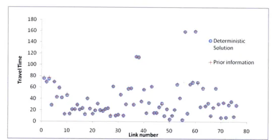
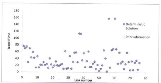
Figure 4-1 shows the solution to the deterministic problem and the corresponding prior travel time on each link. The total error, or the L1 distance from the solution

to the prior information (I|c* - |11), is very small.

Robust problem 180 160 140 0 Deterministic Solution 120 100 + Prior information 80 60 60 0 4 0 40

*

-Set E1:

Consider the case when u = -0.05i and 1 = O.16 (Note that when 1 + u = 0, the deterministic and robust solutions are the same).

180 160 160 9 150 140 0 Robust Solution 140 120 100 + Prior information Ei ~20 80 110 60 0 80 41 110 40 . 8 100 8 10 20 3050 60 7 80 90 20 8 8 880 8880~ 0 ~48 0 0 _{10 20} 2 _30Link 0 _number40 50 00 70 80

Deterministic SolutionR MoTust Solution

(a) (b)

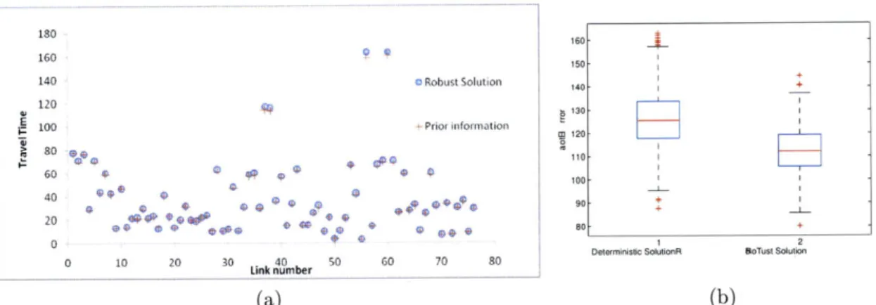
Figure 4-2: Robust solution (a) for Set E1 and box plot (b) for 1000 cases

Figure 4-2a shows the result for the robust problem. We also sample 1000 points

E E E1 from the uncertainty set and plot the box-plot for the total errors of sampled

scenarios

(||c*

(||c*

||1)

-Set E2:

Figure 4-3 shows the solution for the uncertainty set E2.

Interestingly, all of our simulation results for the Sioux Falls network suggest that the result for the robust problem is the same as the result for the deterministic problem. Only for networks with a small number of links, we can observe the differences between the two solutions.

-Set E3:

The stopping criteria for the decomposition algorithm is ub - lb < 0.5%lb.

Figure 4-4 shows the solution and the box-plot for 1000 samples when B = 140. Clearly, the robust solution provides a better mean and variance for the sampled

J-180 160 140 120 E 100 80 60 40 20 0 0 0 Deterministic Solution + Prior information 0 * 04 10 20 30 40 50 60 70 Link number

Figure 4-3: Robust solution for Set E2 when B = 50. Total error = 20. scenarios. 0 Robust Solution -Prior information * * 0 49 4191 0 0 2 4 0 ; L 0 e*,0 0 10 20 30 40 50 60 70 s0 Link number 180 160 140 120 100 60 40 20 +_

Determinislic Solution Robust Solution

(a) _(b)

Figure 4-4: Robust solution (a) for Set E3 and box plot (b) for 1000 cases when

B = 140

Figure 4-5 shows the total error of the worst case and the nominal total error for the deterministic and robust solutions and when the uncertainty budget change. The worst case total error for the deterministic solution increases as the budget increases. On the other hand, the worst case total error for the robust solution increases with a decreasing rate and stables after a while. The nominal error for the robust solution decreases and then stables for the robust solution. This is an attractive property of the robust solution.

100 150 Uncertainty Budget

Figure 4-5: Worst case error (a) budget

and nominal case error (b) with varying uncertainty

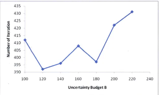
For this network, the dimension of the uncertainty set is 76. In order to solve the problem to optimality, we need to visit all extreme points of this uncertainty set. However, the decomposition algorithm stops after visiting only around 400 extreme points. This is rather efficient for large-scale problems.

120 140 160 180

Uncertainty Budget B

200 220 240

Figure 4-6: Number of iteration with varying budget B

Parametric travel times

In this section, we use 50 historical data points (H = 50). Linear separable travel times :

-+-Robust -I-Deterministic 290 280 270 o 260 250 240 230 220 -4-Robust -- Determini stic 150 Uncertainty Budget 200 200 435 430 425 420 415 410 405 400 395 390 100 .. ...

In this part, to run our simulation, we assume the travel times have the form: c (f) = aZ

fi+b.

leij

L can be thought of as an uncertainty level.

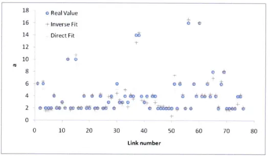
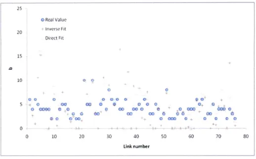
Figures 4-7 and 4-8 show how to fit parameters a and b for each link when L = 20%. Apparently, the linear term a is fitted closely to the real value. However, there are some differences in fitting the constant term b. This is understandable, as one property of UE is that if we shift the whole travel times on all paths by the same constant, the UE flow does not change.

We also compare the results of our method with the results when we directly fit

18 _{o Real Value} 16 + Inverse Fit 0 14 Direct Fit 66 12 1 0 8 0 4b 6+ + 4 V) 0d)000 66b 0~ 0 10 20 30 40 50 60 70 80 Link number

Figure 4-7: Parameter a when L 20%

a curve to the given data. Figure 4-9 shows the total squared error of the fitted travel times and real travel times cr over all H given flow

(ji

BPR travel times:

In this case, the actual travel time function for the simulation will be: e = a

f

[8].

25 20 0 Real Value Inverse Fit Direct Fit 00e 0O0 0 5 +0 00 0 0 0 ,00 0 0 0 0 0 0 ID G 000 o 0a0 + 0+ 0 0 00 ~+ 0 10 20 30 40 50 60 70 80 Link number

Figure 4-8: Parameter b when L 20%

4000 3500 _{-+-Inverse Fit} 3000 -4-Direct Fit 0 2500 2000 - 1500 1000 500 0- - ---- ---0 5 10 15 20 Uncertainty level L

Figure 4-9: Fitting total squared error with varying uncertainty level(%)

travel time with the BPR general form:

ci- = ai3

fP

where a2j, bij, and p are unknown parameters.

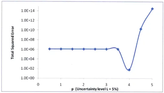
First, we will fix p. Then, a linear regression will be employed in order to find aij, bij and the total squared error to the given data. The value of p with the smallest total

error will be chosen. By scanning p in [0.5 5], step size 0.5, the result in Figure 4-10 1.OE+14 1.OE+12 2 1.OE+10 1.OE+08 O1.0E+06 0 1.E+04 1.OE+02 1.OE+00 -0 1 2 3 4 5 p (Uncertainty level L = 5%)

Figure 4-10: Fitting total squared error with varying p(L = 5%)

shows that p = 4 is the best value.

Figures 4-11 and 4-12 show the parameter a and

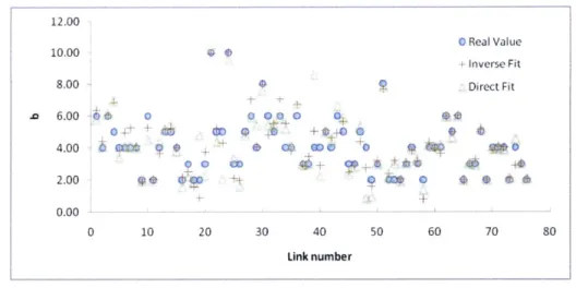
10%. It shows that we can recover pretty well

algorithm. 1.E-14 0 10 20 30 40 1.E-15 _#dl* 1.E-16 dit el 1.E-17 1.E 01 1.E-18 1.E-19 Link number

b when the uncertainty level L =

the parameters using our inverse

50 60 70 80 0 1 *4 0 9 0 Real Value + Inverse Fit Direct Fit

Figure 4-11: Fitting parameter a when L=10%

Figure 4-13 shows the total squared error of the fitted travel times and real travel times cr over all H given flow with varying uncertainty level. It shows that when the uncertainty level is small, the direct fitting and the inverse fitting is quite similar. However, when the uncertainty level gets bigger, the inverse algorithm provides much

0 Real Value + Inverse Fit Direct Fit 12.00 10.00 8.00 6.00 4.00 2.00 0.00 0 10 20 30 40 Link number 50 60 70 80

Figure 4-12: Fitting parameter b when L=10%

better results.

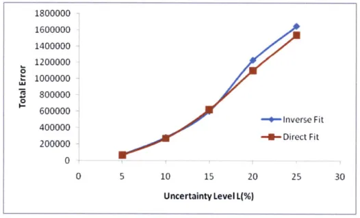
Figure 4-13: Total squared error with varying uncertainty level L (%)

Asymmetric travel times

We further apply our approach to a network (Network 1) with asymmetric travel times (see Figure 5-1 and Table 5.2). Table 4.1 shows the functional travel times found by the inverse optimization method. We can recover quite well the linear terms in most of the links.

In this case, we cannot recover the correct travel times for some of the links. When the uncertainty level increases, it is really hard to recover the underlying travel time

3 00 g& 0 ,' 0000 & 4- 0 S$$ S 90 ~ + C ~ e # 3000 2500 -4-Inverse Fit 2000 --- Direct Fit LU 1500 0 1000 500 0 0 5 10 15 20 25 30 Uncertainty level L (%)