An analog probability density analyzer

DOCUMENT RO {[lIDQ T ROOM 36-412

,-S.ARCUF.I, 'ATOY ' F ....-..

MASSAC'U.-L: .I ' i-.- . ... 1

AN ANALOG PROBABILITY DENSITY ANALYZER

HUGH E. WHITE

TECHNICAL REPORT 326

APRIL 29, 1957

. .0 .

RESEARCH LABORATORY OF ELECTRONICS

CAMBRIDGE, MASSACHUSETTS

4,

_ -I _ _ _

The Research Laboratory of Electronics is an interdepartmental laboratory of the Department of Electrical Engineering and the

Department of Physics.

The research reported in this document was made possible in part by support extended the Massachusetts Institute of Technology, Re-search Laboratory of Electronics, jointly by the U. S. Army (Signal Corps), the U. S. Navy (Office of Naval Research), and the U. S. Air Force (Office of Scientific Research, Air Research and Devel-opment Command), under Signal Corps Contract DA36-039-sc-64637, Department of the Army Task 3-99-06-108 and Project 3-99-00-100.

MASSACHUSETTS INSTITUTE OF TECHNOLOGY RESEARCH LABORATORY OF ELECTRONICS

Technical Report 326 April 29, 1957

AN ANALOG PROBABILITY DENSITY ANALYZER Hugh E. White

This report is based on a thesis submitted to the Department of

Electrical Engineering, M. I. T., April 30, 1957, in partial

ful-fillment of the requirements for the degree of Master of Science.

Abstract

The development and construction of an analog analyzer for determining the first-order probability density function of signal amplitudes of frequencies between 30 cps and 20 kc is described. Values of probability density are determined by averaging a derived random variable that is unity when the signal is in the amplitude interval that is being analyzed and is zero at all other times. It is generated by a diode level-selector circuit that gates a 60-minc carrier to a bandpass amplifier. This level selector eliminates many of the problems of frequency response and drift that are associated with the ampli-tude discriminators of the conventional level selector. The ampliampli-tude range of the signal comprises 50 intervals that are analyzed sequentially and the complete probability density function is plotted by a pen recorder. The frequency response and drift stability of the analyzer are experimentally evaluated, and examples of experimental probability density functions are given.

Block diagrams and descriptions of both digital and analog systems that have been previously developed for determining probability density functions are presented. Definitions and some properties of probability density functions are

i

I. PROBABILITY DENSITY FUNCTIONS 1.1 DEFINITIONS

The definitions of probability density functions assume that a stationary process is evaluated, or that the statistics of the process are not a function of the time of measure-ment. The definitions of the higher-order probability density functions follow directly from the definitions of the first-order and second-order functions given below.

The first-order probability density of amplitude x1 of a function x(t) is the proba-bility that x(t) will have a value between xl and x1 + dx at time t. Since, by definition, this probability is independent of the time of measurement,

P(x ₁ < x(tl) < x₁ + dx) = P(x ₁ < x(t) < x₁ + dx)

In terms of a finite amplitude interval, the first-order probability density of amplitude x is defined as

P(x1 - x(t) < x1 + Ax)

p(x 1) = lim Ax

Ax-o0

The second-order probability density function is the joint probability that the wave-form x(t) will be in the amplitude interval xl to xl + dx at time t1, and in the interval x2 to x2 + dx at time t2 . If times t1 and t2 are separated by T seconds, and the joint probability is independent of the time of measurement, we have

P [(x1 x(tl) < xI + dx);(x2 < x(t2) < x2 + dx)] = P [(x1 x(t) < x1 + dx);(xz < x(t+ T) < x2 + dx)]

The second-order probability density for finite intervals is defined similarly to the first-order density as follows:

P[(x1 Xx(t) < x1 + A 1); (x2 < x(t + T)< x2 + Ax2)]

PZ(x1 x2 T) = lim Ax Ax

Ax -O 1

Ax -10

1. Z2 METHOD FOR DETERMINING PROBABILITY DENSITY

A convenient method for experimental determination of the probability density of amplitude x is to generate a derived random variable that is unity when x1 < x(t) < x1 + Ax, and zero at all other times. The time average of this derived

random variable is equal to the probability density of amplitude x. Since this relation is utilized in several analyzers that are described in Section II and by the analog proba-bility density analyzer, a proof similar to Davenport's (3) will be given.

The derived random variable, u(t), is defined by the relations

INTRODUCTION

The application of statistical methods to the study of communication systems has resulted in the improvement of existing systems and the development of new systems. The pioneer in the field of statistical communication theory is Norbert Wiener (14). Statistical methods allow the communication engineer to characterize the messages that will be transmitted by a communication system. The system can then be optimized for transmission of the desired messages, or the statistics of the messages can be varied to complement an existing system. A whole class of probability density functions is required to completely characterize a random process. Useful results, however,

may be obtained from a knowledge of the first-order or of the first- and second-order probability density functions, which are relatively simple to evaluate. The problem to be considered is the development of an analog density analyzer for the experimental determination of the first-order probability density function.

The first section of this report is concerned with definitions and characteristics of the probability density functions. Block diagram descriptions of previously

con-structed equipment for the determination of probability density functions are presented in Section II. The analog probability density analyzer is described in Section III in block diagram form, and then the circuits of the block diagram are described in

de-tail . Experimental results, including frequency response and stability characteristics, are presented in Section IV which concludes with a discussion of possible analyzer modifications.

if x <x(t) < x1 + Ax u(t) =

0 otherwise

The statistical average, u, of the derived random variable is

U =f upl(u)du

Since u contains only the values zero and one, Pl(u) consists of two impulses. The statistical average of u can, therefore, be represented as the summation

u = uj P(u =uj) j=O

which, when it is evaluated, gives u = P(u=l)

Returning to the definition of the derived random variable, we see that P(xl < x < x1 + Ax) = P(u=l) = u. The desired probability is equal, therefore, to the statistical average of the derived random variable.

By definition, the statistical average of u(t) implies the simultaneous measurement of all the member functions of an ensemble of u(t). Since it is not convenient to

measure a statistical average experimentally, it is desirable to relate the statistical average of u(t) to the time average of one member of the ensemble. The ergodic theorem for stationary random processes states that the statistical average taken over the entire ensemble is equal to the time average of one member of the ensemble over an infinite interval. The probability density pl(xl) is proportional, therefore, to a time average of the derived random variable as the interval width, Ax, approaches zero.

1.3 PROBABILITY DISTRIBUTION RELATED TO PROBABILITY DENSITY

The probability distribution function is the integral of the probability density func-tion. The probability distribution of amplitude x is the probability that x(tl ) is less than x1, and, for a stationary process,

P[x(tl) < x] = P[x(t) < xl]

The simpler definition of the probability distribution function simplifies its experimental determination, as compared with the probability density function. For this reason, experimental studies have been made of probability distributions, and in some instances probability density has been calculated from experimentally determined probability distribution functions.

1.4 PROBABILITY DENSITY OF THE SUM OF TWO VARIABLES

An important relation exists between the probability density of the sum of two inde-pendent functions and the densities of the separate functions. If z(t) is the sum of the two variables x(t) and y(t), and p(z), Pl(x), and p2(y) are the corresponding probability densities, then

p(z) =

f

Integrals of this form, known as "convolution integrals," are encountered in finding the response of a linear network in the time domain. The alternative method of deter-mining network response in the frequency domain suggests itself as an alternative means of finding p(z). This is accomplished by taking the Fourier transform of the probability densities pl(x) and p2(y) to form their respective characteristic functions.

The inverse Fourier transform of the product of the characteristic functions is p(z), the probability density of the sum of the random variables x and y.

II. REVIEW OF PREVIOUSLY CONSTRUCTED EQUIPMENT 2. 1 BASIC EQUIPMENT CONSIDERATIONS

Before describing specific analyzers it will be helpful to consider two basic prop-erties that would have to be taken into account in describing any probability density

analyzer. The first is related to the resolution of the analyzer, that is, how closely the output of the analyzer approximates the theoretical probability density. In the major-ity of the analyzers that will be described the total amplitude range of the signal is

divided into a number of amplitude intervals, x, which are analyzed separately. To obtain the theoretical probability density, however, it would be necessary to use an infinite number of infinitesimal intervals, as is indicated by the definition of Pl(x) given in section 1. 1. Hence, the resolution obtainable with any analyzer is proportional to the number of amplitude intervals used. In some analyzers, such as the probabiloscope that will be described, it is difficult to determine the exact number of intervals; but in an

electronic analyzer it is simply the ratio of the peak-to-peak voltage amplitude of the analyzed signal to the voltage width of the amplitude interval.

The second property concerns the manner of analyzing the amplitude intervals. Since most analyzers are designed for stationary processes, it is possible to analyze the intervals sequentially and obtain the same result that is obtained by analyzing the inter-vals simultaneously. The sequential analyzer requires much less equipment than the simultaneous analyzer, but it does require a scanning system to select the various amplitude intervals for analysis. A simultaneous analyzer requires sufficient dupli-cation of equipment to analyze all intervals simultaneously, which results in a reduc-tion of the total analysis time, as compared with the sequential analyzer.

Description of the probability density analyzers will also be facilitated by explaining the function of two circuits that are used in several of the analyzers. The first is the slicer circuit which is a form of amplitude discriminator. The slicer circuit has zero outputwhen its input signal is less than the preset slicing level, and unity output when the input signal is greater than the slicing level.

The second circuit is the level selector which is another form of amplitude discrim-inator. A unity output is obtained from the level-selector circuit whenever the input signal is within some preset amplitude interval, and zero output is obtained if the input is greater or less than the bounds of this amplitude interval. The output of a level-selector circuit corresponds to the derived random variable, u(t), described in section 1. 2.

2. Z2 ANALOG PROBABILITY DENSITY ANALYZERS

A great variety of analog systems has been developed for determining probability density. Analyzers that determine probability density by averaging a derived random variable have already been mentioned. Probability density functions have also been

obtained by using a storage tube (12) or photographic film (15, 10) to record the presence of the signal directly in a particular amplitude region. In general, analog methods of determining probability density require simpler equipment and produce less exact results than digital methods. A review of three analog probability density analyzers is presented in the following sections.

a. Probabiloscope

A study of the statistics of television signals was accomplished with the aid of the probabiloscope (10) which uses a simultaneous photographic method for obtaining the probability density function. This system has the advantage of excellent frequency response, but it requires special photographic processing to develop the exposed film.

A diagram of the probabiloscope is shown in Fig. 1. The cathode-ray spot is

deflected by the television signal, and the average dwell time at any point is proportional

to the probability density of the corresponding amplitude. The point source of light is

mapped into a vertical line by the optical system before passing through the optical-density wedge to the film. Since the optical-optical-density wedge tapers the light transmission

as a function of height, the film is exposed to a height that depends on the average dwell time at a corresponding amplitude. The desired probability density is recorded on the film as contours of constant exposure that can be changed to a sharp line by special photographic processing.

b. Direct-Reading Probability Distribution Meter

The probability distribution meter (4) is a sequential analyzer that presents values of probability density on a calibrated meter. Scanning of the amplitude intervals is

accomplished by the operator, who controls a potentiometer dial calibrated in ampli-tude units.

As shown in Fig. , the scanning potentiometer is associated with the

cathode-coupled clipper circuit. The function of the clipper circuit is to amplify that part of the input waveform which includes the interval selected for analysis. Direct-current refer-ences are provided for the two slicer circuits by clamping the clipper output signal to fixed voltages. The slicing levels are set to differ by 7. 5 volts, which, with the gain available in the amplifier and cathode-coupled clipper circuit, divides the signal into

100 intervals. The difference of the integrated outputs of the two slicer circuits is registered on a dc voltmeter. This average is equivalent to the average of the derived random variable, u(t), and it is proportional to the probability density.

Small drifts of the gain of either channel of the probability distribution meter will cause a relatively larger drift of the meter zero, since the difference of two large quantities is read by the dc voltmeter. Satisfactory high-frequency operation of the distribution meter is dependent on achieving identical rise-time characteristics between the two channels. This requires equal capacities at various points of both channels. Although the probability distribution meter has been described as being

HMIH 1KANSMISSION LIGHT- PROOF ENCLOSURE

Fig. 1. The probabiloscope.

Fig. 2. Direct-reading probability distribution meter.

(a)

23 23

x(t) LEVEL INTEGRATOR SEQUENTIAL OSCILLOSCOPE

SELECTORS CIRCUITS - SAMPLER

(b)

Fig. 3. (a) Electronic amplitude probability distribution analyzer.

(b) Revised form of Fig. 3a.

useful for frequencies up to 100 kc, it was also mentioned that the density distribution of a sine wave will shift in position and amplitude for high frequencies.

c. Electronic Amplitude Probability Distribution Analyzer

The electronic amplitude probability distribution analyzer (6) is a simultaneous probability density analyzer that operates on a short-time basis for the analysis of nonstationary processes. The analyzer presents the probability density of the input waveform for some interval T in the form of an oscilloscope display of a 12-point histogram.

The block diagram of this analyzer, shown in Fig. 3a, indicates the duplication of equipment that is necessary to simultaneously analyze twelve amplitude intervals. The binaural recorder provides a delay between the two channels that is equal to the desired analysis time T. A channel output consists of the output of 12 level-selector circuits that cover the amplitude range of the signal. At any instant, only one level selector, the one containing the signal in its amplitude interval, has a nonzero output. Both channel outputs are identical, with the exception of the delay introduced by the recorder and the polarity inversion of the delayed channel. The sum of the averaged level-selector outputs of corresponding intervals of the direct and delayed channel is proportional to the percentage of time that the signal remains in the interval during the analysis time. This may appear more evident if it is realized that the inverted delayed channel is subtracting pulses from the integrator which were placed there T seconds earlier by the direct channel. The pulses that remain in the integrator are, therefore, those placed there by the direct channel during the delay period T. The voltages of the 12 integrators are periodically sampled and displayed on an oscilloscope.

The frequency response of the analyzer was experimentally determined as from 20 to 50 cps, with a 5 per cent error. Drift of the amplitude discriminators contained in the level-selector circuits, however, precluded meaningful results a few minutes after alignment.

The equipment of the electronic amplitude probability distribution analyzer has been revised (see Fig. 3b) in a form that has yielded more useful results (16). The principal change involved in the revision is that the delayed channel was eliminated, and the delayed-channel equipment was used to extend the number of amplitude intervals to 23. Each of the amplitude intervals is terminated in a resistor-capacitor integrator, and the analysis time is varied by changing the integrator time constants. The drift stability of the analyzer was improved by eliminating the delayed channel, and the

revised short-time probability density analyzer was successfully used for the analysis of radar signals for an extended period of time.

2.3 DIGITAL PROBABILITY DENSITY ANALYZERS

Since both analog and digital probability density analyzers are designed to operate with a continuous input signal, a means of converting the continuous signal to digital

Fig. 4. Probability density analyzer Fig. 5. Level-selector circuit. for speech analysis.

form must be included in the digital analyzer. The operations performed on digital information may be considered exact, and, therefore, the elements that are of interest in the digital analyzer are those used for analog-to-digital conversion. In the following descriptions of digital analyzers emphasis is placed on the equipment that is used to obtain a digital representation of the signal.

a. Probability Measuring Equipment for Speech Analysis

Digital equipment for the measurement of first-order and conditional probability density was developed for a study of speech waves (3). Davenport describes his choice of digital equipment for measuring probability density as a means of facilitating the

measurement of the conditional probability density. This is a result of the simple storage processes for digital information that are used in the conditional probability delay unit.

The analyzer used to measure the first-order probability density is shown in Fig. 4. The functions of the various items of equipment will now be described. The sampling pulse generator produces a series of equally spaced, constant-amplitude pulses. The

amplitude of these pulses is varied in proportion to the amplitude of the voice wave at the sampling instant by the pulse-amplitude modulator. The function of the level selector

is to produce an output pulse only when the amplitude of an input pulse falls between

x1 and x + ax.

The probability density of a particular amplitude, x, is determined by the relation

P(x 1 x < x1 + Ax1) = lim lim- _

T-'oo n-oo n

where n is the number of pulses generated, and v is the number of pulses whose

ampli-tudes fall between x1 and xl + Ax. While the desired value of probability would be

obtained for only an infinite number of samples and for an infinite interval, the error can be made small by choosing large finite values of T and n.

The level selector consists of two slicer circuits and an anticoincidence circuit, as shown in Fig. 5. The slicer circuits are set to amplitude levels that differ by 10 volts, and, since the analyzer is designed for 100 levels, it is necessary to introduce a

9

1000-volt variation of pulse amplitude into the level selector. This is accomplished by slicer amplifiers which are similar to the cathode-coupled clipper used in the proba-bility distribution meter. The 10-volt amplitude interval was chosen to make the varia-tion of the discriminavaria-tion level of the slicer circuits approximately 5 per cent of the amplitude interval width.

The duration of the sampling pulse determines the maximum signal frequency that can be sampled, since the signal should not vary more than one amplitude interval during the pulse duration. On this basis, it can be shown that when 100 amplitude inter-vals are used, a maximum frequency of 6. 8 kc may be sampled with the 0. 5-4sec pulse used by the system.

b. Noise Distribution Analyzer

A study of filtered random noise was performed with a noise distribution analyzer (9) that determined the probability distribution of the noise envelope. The probability

density of the noise envelope was then calculated from the distribution function.

A block diagram of the noise dis-tribution analyzer is shown in Fig. 6. Output pulses are generated by the one-shot multivibrator whenever noise peaks ,exeeP d the disc.rimination level

deter-Fig. 6. Noise distribution analyzer. mined by the scanning circuit. The sum

Fig. 6. Noise distribution analyzer.

of these constant-duration pulses is dis-played by the counter for a sampling period determined by the timer. The scanning circuit of the noise distribution analyzer consists of 28 dry-cell batteries connected in series and a switching arrangement to select the desired discrimination level of the one-shot multivibrator. Since precision resistors are included to change the discrimination level in steps of either 1/3 or 1/2 of a dry-cell battery, a maximum of 84 amplitude intervals is used by the analyzer.

The probability distribution of amplitude x1 is # counts (xl)

P(x ₁) = 1

-# counts (0)

where # counts (x1) is the counter sum over the sampling period at amplitude x1, and # counts (0) is the counter sum at zero amplitude over an equal sampling period. The probability density for amplitude x, which is bounded by xl and x2, is given by

# counts (x₁) - # counts (x₂)

p(x) = x -x

x2 - ₁

An equipment test of the noise analyzer was performed by finding the probability

Fig. 7. Digital probability density analyzer.

distribution and probability density of the envelope of a 16. 4-kc carrier amplitude mod-ulated by a 400-cps sine wave. This method of determining probability density is similar to that used by the speech-density analyzer described in section Z. 3a, if the amplitude-modulated carrier is considered equivalent to the output of a pulse-amplitude modulator.

c. Digital Probability Density Analyzer

The digital probability density analyzer (7) differs from the other digital systems that have been described in that amplitude samples of the signal are converted into pulse-time modulated samples previous to quantizing by an interval-selector circuit. The digital analyzer operates in conjunction with the M. I. T. digital correlator (13) which

generates the pulse-time modulated samples. The correlator samples consist of groups of two pulses which are separated by a time interval that is proportional to the signal

amplitude at the sampling instant. The correlator must obtain two amplitude samples,

separated by a time interval, T, in order to calculate a sample of the correlation

function. The correlator samples are also suitable for determining the second-order probability density function.

A block diagram of the equipment for determining the first probability density is shown in Fig. 7. The function of the interval selector is to produce a pulse output

when-ever an input pulse falls between t and t1 + At. If amplitude samples of the input signal

whose amplitudes fall between x1 and xl + Ax produce time-modulated pulses separated

by time intervals between t1 and t + hAt, the probability density of amplitude xl is

pro-portional to the counter sum over the sampling period. The sampling period is the inte-gration time of the digital analyzer and it is determined by the correlator timing circuits. Various sampling periods are available, but the period is not changed while the 50 inter-vals of one density function are being analyzed. The frequency response of the digital

analyzer is determined by the response of the sampling circuits of the correlator which extend from a few cycles to one megacycle per second.

11

III. THE ANALOG PROBABILITY DENSITY ANALYZER 3. 1 BLOCK DIAGRAM DESCRIPTION

The analog probability density analyzer is a sequential system for determining the first-order probability density function. The frequency response of the analyzer is from

30 cps to 20 kc, and no analyzer drift is present for periods greater than the maximum analysis time of a probability density function. Probability density is determined by the method of averaging a derived random variable, as described in section 1. 2, and the

complete density function is plotted by a recording ammeter.

A diode level selector, shown in the block diagram of Fig. 8, generates the derived random variable. The level selector functions as a switch that connects the 60-minc

oscillator to the bandpass amplifier whenever the value of x(t) lies between x₁ and

x₁ + Ax. The derived random variable is therefore generated in the form of 60-minc

pulses. The circuitry that follows the diode level selector is required to modify the level-selector output before averaging and plotting by the pen recorder. Analysis of the 50 amplitude intervals comprising the amplitude range of x(t) is accomplished by the scanning system. A scanning signal, synchronized with the paper position of the pen recorder, varies the dc level of x(t) to permit the level selector to analyze each inter-val. A further description of the analyzer circuitry is divided into three parts: the level-selector circuit, the pulse circuitry and integrator, and the scanning system. A

complete circuit diagram of the analog probability density analyzer is given in Figs. 9 and 10.

3.2 LEVEL-SELECTOR CIRCUIT

The analog probability density analyzer uses a diode level selector to generate the derived random variable. The diode level selector eliminates the difficulties introduced by the slicer circuits of the conventional level selector. Drift of the interval boundaries is not a problem with the diode circuit, and high-frequency operation is not sacrificed by slicer-circuit unbalance. Another source of level-selector drift is eliminated, because it is not necessary to take the difference of two slicer-circuit outputs to obtain the derived random variable.

The present series-diode level selector has evolved from a shunt-diode circuit which was first suggested by A. G. Bose (2). One of the diodes of the shunt circuit, shown in Fig. 11, will conduct whenever the input signal x(t) is outside the amplitude

interval of +AE/2 to -E/Z, but neither will conduct when the signal is within the

ampli-tude interval. The shunt diodes, therefore, act as a switch which closes to shunt the high-frequency carrier to ground through the impedance of the x(t) signal source. An experimental difficulty encountered with the shunt-diode circuit was the realization of an x(t) signal source with a low 60-minc impedance. This resulted in an appreciable leakage of the 60-minc carrier to the bandpass amplifier when the diodes of the shunt level selector were conducting.

Fig. 8. Block diagram of analog probability density analyzer.

20,000 OHM

360' ROTATION

I% LINEARITY

SCANNING POTENTIOMETER (GEARED TO PEN RECORDER)

Fig. 9. Level-selector circuit and scanning system.

Fig. 10. Bandpass amplifier, detector, clipper, and integrator circuits.

13

TO BANDPASS

AMPLIFIER

-Ek 60-MC

OSCILLATOR

Fig. 11. Shunt-diode level selector. Fig. 12. Series-diode level selector.

Fig. 13. Simplification of series-diode level selector.

c

OUTPUT STAGE OF BANDPASS AMPLIFIER

Fig. 14. Detector circuit.

14 TO BANDPASS B+ AMPLIFIER -Ek 60-MG OSCILLATOR x (

The series-diode level selector, shown in Fig. 12, has largely eliminated the prob-lem of level-selector leakage; hence this is the circuit used in the analog probability density analyzer. A small level-selector leakage signal is present in the series circuit because of capacitive coupling across the diodes during periods of nonconduction. This leakage, however, can be eliminated by the cutoff bias of a pulse amplifier that follows the level selector. Comparison of the circuit diagrams of the series-diode and the shunt-diode level selectors reveals that the two circuits are dual in some respects. This is true because the diodes of the series circuit are conducting during the pulse duration, while the diodes of the shunt circuit are nonconducting, and a high-impedance carrier source is switched by the shunt circuit and a low-impedance source by the series

cir-cuit. Determination of the optimum element values for the level selector is accomplished by analyzing the circuit requirements with respect to the three input signals and the single output signal. The level-selector input signals are: the signal to be analyzed,

x(t), the high-frequency carrier, and the dc bias, E. The single output signal, which

is a function of the three inputs, is the derived random variable.

When we analyze the level-selector circuit with respect to the input signal, x(t), the circuit of Fig. 13 may be used. Depending on the time constant of the RC combinations, the diodes of this simplified circuit can function as clippers, or peak detectors, or as a circuit intermediate between these extremes. For proper operation of the level-selector circuit, however, the diodes must function as clippers; and therefore it is

necessary to choose small values of Cc and RL.

The lower bound of possible values for the RL's is determined by their effect on the operating path of the cathode-follower signal source. Since the value of RL that is used in the level selector is of the same order of magnitude as Rk, it is necessary to include the RL's when determining the operating path of the cathode follower. The cathode-follower operating path is of interest because the intersection of the operating path with the zero-bias plate characteristic determines the maximum positive cathode-follower grid voltage that is possible without grid current. This value of grid voltage is the prod-uct of the tube current at the given intersection and the parallel resistance of Rk and one RL. Since the cathode resistor of the cathode follower is returned to the negative voltage Ek, the maximum positive grid-to-ground voltage is Ek volts less than the maximum grid voltage.

The two bias batteries, E/Z, determine the voltage width of the level-selector

amplitude interval. To minimize the required amplification of x(t), it is desirable to use a small voltage interval, but to realize good diode switching it is necessary to avoid the curved part of the characteristic of the diodes. Drift of the boundaries of the amplitude interval need not be considered in determining the interval voltage, however, since the width of the interval is accurately maintained by battery bias. A voltage inter-val of three volts was chosen for the series-diode level selector by examining the wave-form of the level-selector pulse output. This choice is convenient, because small flashlight batteries can be used for the two bias batteries AE/2.

15

Careful examination of the level-selector circuit reveals that the voltage interval is not entirely determined by the sum of the two bias batteries, AE. The actual voltage interval is slightly greater than AE because an additional bias is developed by diode current flowing through the output impedance of the cathode follower. The polarity of this bias depends on which diode is conducting, but in both cases the bias has the proper polarity to add to the bias source, AE/Z, of the nonconducting diode. Since the cathode-follower output impedance is small, the bias developed in this impedance is small com-pared with the battery bias, AE.

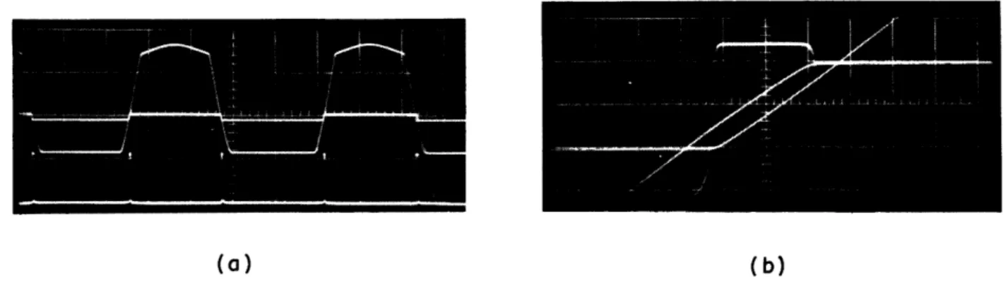
The total magnitude of the voltage interval may be measured on a dc oscilloscope by comparing the clipping level of the two diodes. Triple-exposure oscillograms taken with external synchronization, Fig. 15, show the clipping level of the two diodes and the resulting pulse output from the detector. These oscillograms show that the difference of the diode clipping levels determines the duration of the generated pulse. A determination of the total voltage interval is required when the gain of the x(t) amplifier is set to uti-lize a certain number of amplitude intervals.

The 60-minc path of the series-diode level selector consists of the two diodes and the two coupling capacitors. This path is isolated from the bias sources by the diode load resistors and from the signal source by the rf choke. The coupling capacitors that separate the bias and 60-inc signals have a small value for minimizing the time con-stant RLCc that was considered before. Since these capacitors must have a low imped-ance at the carrier frequency, the advantage of choosing a high-frequency carrier is evident. The voltage of the 60-inc oscillator is small compared with the voltage inter-val, AE, in order to prevent the carrier signal from influencing diode conduction. Since

amplification of the level-selector output is equivalent to switching a large carrier voltage, this does not represent a restriction.

3.3. PULSE CIRCUITRY AND INTEGRATOR

The circuitry following the level selector in the analog probability density analyzer determines the average of the derived random variable generated by the level selector.

Before integration it is necessary to modify the level-selector output in order to obtain a useful output signal from the integrator circuit. First, the pulses of the 60-inc

car-rier are amplified by a bandpass amplifier to provide sufficient integrator output for the operation of the pen recorder. Detection of the 60-minc pulses is required to produce video pulses with a nonzero average. Then, the video pulses are clipped and a small

level-selector leakage signal is removed to produce a better approximation to the derived random variable described in section 1. 2. Clipping is required to remove var-iations in pulse amplitude that could be introduced by changes of carrier amplitude or amplifier gain. The level-selector leakage signal is a small voltage that is present between pulses which must be removed to eliminate its contribution to the pulse average.

Finally, the derived random variable is averaged by a resistor-capacitor integrator, and the integrator voltage which is proportional to the probability density is plotted by

(a) (b)

Fig. 15. Waveforms of level-selector circuit (taken at points A and B of Fig. 12) and

detector pulse output (taken at point C of Fig. 14). Figure 15b is an expanded view of one intersection of Fig. 15a with the pulse waveform superimposed on the level-selector waveform.

the pen recorder. The circuits used to modify and integrate the derived random variable will be described in this section.

The bandpass amplifier was originally designed for radar applications and has a 20-mc bandwidth centered about 60 mc. Nine type 6AK5 stagger-tuned amplifiers vide an even response within the band limits of 50 to 70 mc. The large bandwidth pro-duces a short amplifier rise-time which is required to amplify short-duration pulses. If amplifier rise-time is defined as the response time to a step input, amplifier rise-time

1

and bandwidth are related by tc 2.2 where t is the amplifier rise-time, and f

the bandwidth. Thus, the minimum possible rise-time at the output of the 20-mc band-width amplifier is 0. 025 Lsec. The amplifier gain is controlled by varying the grid bias of the second, third, and fourth amplifier stages. A schematic diagram of the bandpass amplifier is not included, since the design is conventional.

A type 6AL5 diode is used to detect the 60-minc pulses. The circuit shown in Fig. 14 is similar to circuits used for radar applications and is designed to produce video pulses

with short rise-times. The time constant of RtCt is chosen to be equal to a few cycles

of the carrier frequency. Sixty-megacycle ripple of the output pulses is removed by the filter LfCf.

Amplification of the derived random variable at the carrier frequency provides dc response at the detector output. Thereby, dc amplification is not required after the detector stage, and a source of dc drift is eliminated. Three direct-coupled pulse amplifiers are used to modify the video output of the detector, but, since their gain is near unity, drift is not a problem. Amplification of the averaged derived random vari-able, however, is impossible without introducing drift. Therefore, sufficient amplifi-cation is included before integration to permit direct recording of the integrator output.

The three direct-coupled pulse amplifiers following the detector perform three func-tions: they clip the peaks of the derived random variable to remove amplitude varia-tions, remove the level-selector leakage signal, and provide a current source of pulses

17

____________1_113_____---for the integrator. Two of the three 6AU6 sharp-cutoff pentodes are connected in paral-lel to provide sufficient current for operation of the recording ammeter. All of the pulse amplifiers are operated at a low screen voltage to permit complete cutoff of their plate current by a negative two-volt grid voltage.

The first pulse amplifier is conducting when no pulse is present. A negative two-volt pulse from the detector will drive the amplifier into cutoff and the first pulse amplifier, therefore, clips the peaks of the pulse amplitude. As shown in Fig. 16, the bias of the

second and third pulse amplifiers is

dovlpnn1 senorPncc th n+,_lnnl rcioCnr

of the first amplifier. Cutoff bias is devel-oped across the plate resistor when the first amplifier is normally conducting,

and the level-selector leakage signal is removed by this means. When amplifier V1 is cut off during the pulse interval, the bias of V2 and V3 will be driven to zero; and the resulting plate-current

HIGH B+

pulses of V and V₃ are averaged by the

Fig. 16. Clipper circuits and integrator. integrator.

Pentodes V2 and V3 represent a cur-rent source of pulses, since the amplitude of the plate-curcur-rent pulses is not a function of the integrator voltage. A current source of pulses is required if the integrator aver-age is to be only a function of the averaver-age time a pulse is present. The detector out-put, for example, does not represent a current source, since the integrator voltage will bias the detector. The effect of this bias is to limit diode conduction in proportion to the integrator voltage.

3.4 SCANNING SYSTEM

Since the analog probability density analyzer obtains the probability density in a sequential manner, a scanning system must be included to select the amplitude inter-vals for analysis. To provide a continuous recording of the probability density function of x(t), the scanning system continuously varies the amplitude interval, Ax, over the amplitude range of x(t). The paper position of the pen recorder is synchronized with the scanning system so that a recorded value of probability density can be associated with the correct amplitude. A periodic scanning system is employed by the analog prob-ability density analyzer to provide a continuous repetition of the probprob-ability density function. The incorporation of a scanning system into the analyzer requires, first, the generation of a suitable scanning signal. Second, it is necessary to introduce the scanning signal into the analyzer circuitry in a way that will not interfere with the normal circuit operation.

A continuously rotating single-turn potentiometer is geared to the paper-feed roller

of the recording ammeter to generate the required scanning signal. Since the paper feed moves at constant speed, the resulting signal is a linear saw tooth, and the period of the saw tooth is determined by the gear combination used in the recording ammeter. Gearing the potentiometer to the paper-feed roller of the recording ammeter, rather than to the drive motor, maintains the same amplitude calibration of the recorded probability den-sity function when the recorder speed is changed. The magnitude and voltage level of the scanning signal may be varied to cover any amplitude range by returning the potentiom-eter to voltage sources of proper magnitude. To maintain a linear scanning voltage, connection of the scanning signal to the analyzer circuit must not allow current to flow in the potentiometer slider.

The analog probability density analyzer employs a 20, 000-ohm continuously rotating potentiometer with 1 per cent linearity to generate a saw-tooth voltage that rises from -100 to +100 volts. To avoid the danger of damage to the potentiometer by accidental shorts, the leads connected to the voltage sources are fused with 10-ma fuses.

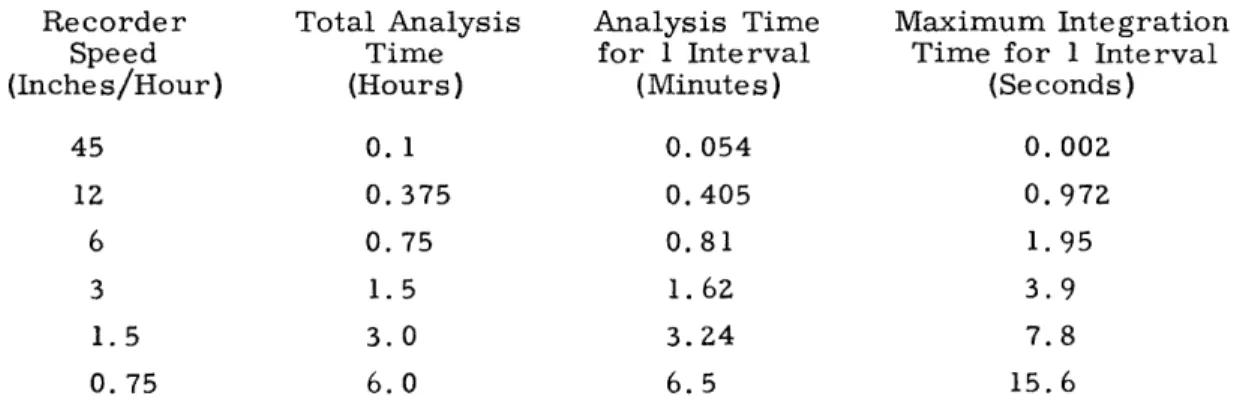
Table I. Analysis and Integration Times of Analog Probability Density Analyzer. Recorder Total Analysis Analysis Time Maximum Integration

Speed Time for 1 Interval Time for 1 Interval

(Inche s/Hour) (Hours) (Minutes) (Seconds)

45 0.1 0.054 0.002 1Z 0.375 0.405 0.972 6 0.75 0.81 1.95 3 1.5 1.62 3.9 1.5 3.0 3.24 7.8 0.75 6.0 6.5 15.6

Five scanning speeds are available by changing gears in the pen recorder. The scanning speed chosen for a given application will depend on the desired integration time for one of the amplitude intervals. The five recorder speeds are listed in Table I, together with the time required to scan one amplitude interval and the total time required to analyze the complete waveform. The duration of the scanning signal within one ampli-tude interval does not equal the allowable integration time for a particular recorder

speed. Since the voltage of the RC integrator must be able to change by large amounts between adjacent intervals, the time constant of the integrator must be short compared with the analysis time of one interval. The actual integration time of the signal is small

compared with the integrator time constant, and the integration time is, therefore, much shorter than the analysis time of the interval. If the integrator time constant is chosen as one-fifth of the analysis time of the interval, and the integration time is assumed to be one-fifth of the time constant, the maximum integration times for each recorder speed can be taken from column 4 of Table I.

As we have mentioned, the introduction of the scanning signal into the analyzer must

19

+30V B+

x(t)

PEN RECORDER) -100V FOLLOWER CATHODE

FOLLOWER

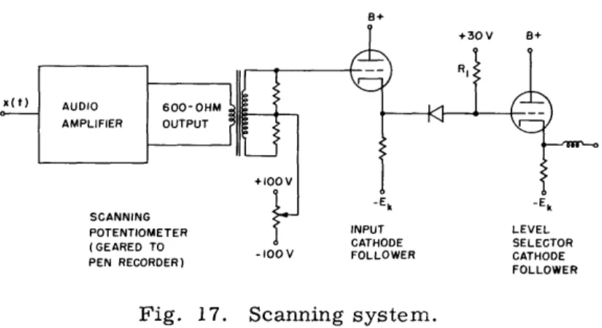
Fig. 17. Scanning system.

not interfere with the proper operation of the analyzer circuitry and must not allow cur-rent to flow in the scanning potentiometer. The choice of a method for connecting the scanning signal to the analyzer circuitry depends on whether an ac or a dc amplifier is used to amplify x(t).

When dc amplification is employed, the scanning signal can be easily introduced into the amplifier. Since differential amplifiers are ordinarily employed as dc amplifiers, the scanning signal and x(t) can be introduced into the separate inputs of a differential amplifier.

The analog probability density analyzer employs an ac coupled signal amplifier. This choice was made to eliminate drift in the signal-amplifier section of the analyzer so that the drift stability of the level selector and the integrator circuitry could be evalu-ated. The use of an ac coupled amplifier requires that the scanning signal be introduced at the output of the signal amplifier, and that the peak-to-peak values of x(t) and the saw-tooth scanning signal are of equal value.

The analyzer scanning circuit, shown in Fig. 17, includes a wide-range audio amplifier to amplify x(t). The 600-ohm output of the amplifier is connected to an input transformer which adds x(t) to the scanning signal in the secondary winding. In addition to providing dc isolation between the amplifier and the scanning voltage, the input trans-former raises the voltage level of x(t) to 200 volts peak-to-peak. The secondary of the transformer is terminated in a resistance to reflect the proper load to the amplifier.

The large variation in the sum of the scanning signal and the amplified x(t) does not allow direct connection to the level-selector cathode follower without introducing grid current. Since the same amplitude interval of the sum of x(t) and the scanning signal is always viewed by the level selector, distortion of other amplitudes is not important; and it is possible to clip large positive excursions of x(t) that would otherwise cause cathode-follower grid current. It is just as objectionable, however, to have clipper current flowing in the scanning potentiometer as grid current. An input cathode follower is therefore included to isolate the clipper current from the scanning source. A large value of cathode resistance and a high-gain triode are used for the input cathode fol-lower to allow large positive grid voltages without grid current. The oscillogram of

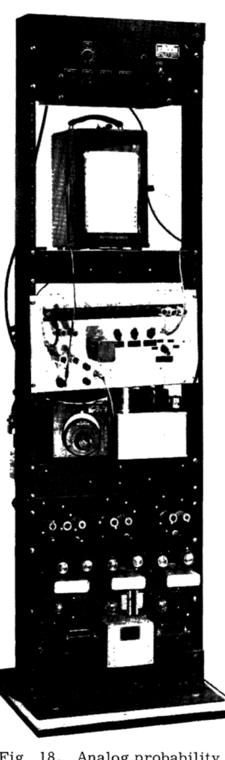
Fig. 18. Analog probability density analyzer.

Fig. 15a shows the waveform of a sine wave after clipping has eliminated cathode-follower

grid current. The chosen value of R1 for the

clipper load resistance is not sufficiently large to provide perfect clipping. Grid current is

eliminated by this value of R1 and response to

high frequencies is not affected.

Further inspection of Fig. 15a reveals that negative excursions of the sine wave are also

clipped. This clipping is a result of the cutoff of both cathode followers for grid voltages

lower than -(Ek+ Ecutoff). The cathode-follower

amplifiers are returned to -Ek to allow linear

amplification of x(t) around ground potential, but

there is no reason to make Ek sufficiently

nega-tive to avoid cutoff, because the level selector only analyzes amplitudes near ground potential. A further reason for clipping both positive and negative excursions of x(t) is to minimize the peak inverse-voltage requirement of the level-selector diodes.

Figure 18 is a photograph of the analog probability density analyzer. The equipment is arranged in the relay rack as follows. The top panel is a noise generator that was used as the signal source for the noise density functions. The upper shelf supports the recording

amme-ter which is directly above the panel contain-ing the level selector, the bandpass amplifier, and the detector and integrator circuits. The lower shelf supports the 60-minc oscillator and the audio amplifier, and the bottom panel con-tains regulated power supplies for the analyzer.

21

--j

IV. EXPERIMENTAL RESULTS

4. 1 EVALUATION OF ANALYZER OPERATION

The first experimental work with the analog probability density analyzer was devoted to evaluating the analyzer operation. The analyzer accuracy was initially checked by comparing the experimental probability density of a sine wave with calculated values.

Further testing was concerned with determining the frequency response and drift stabil-ity of the analyzer.

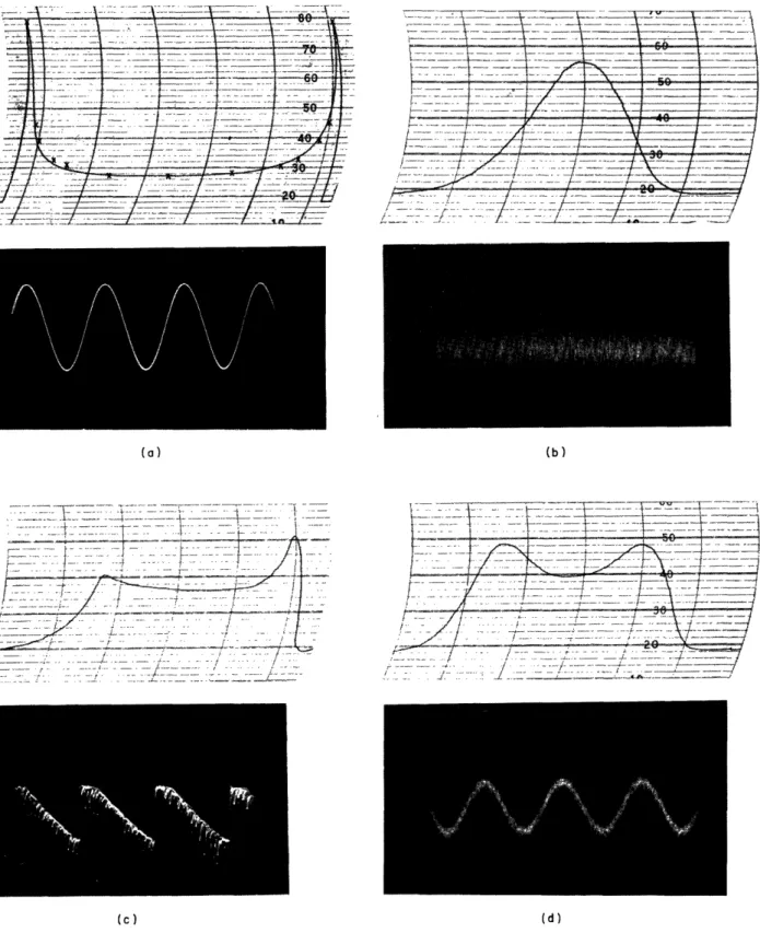
An experimental probability density function of a 1-kc sine wave analyzed by 50 amplitude intervals is shown in Fig. 19a. Calculated values of sinusoidal probability density for 50 intervals are indicated by crosses. Comparison of the experimental curve and the calculated values reveals that error is present in regions in which the slope of the probability density is large. Verification of the fact that this error is produced by the recorder was made by replacing the recorder with a voltmeter. Values of probabil-ity densprobabil-ity read from the voltmeter showed no deviation from the calculated values.

Reversing the sequence of scanning the amplitude intervals, scanning from negative to positive amplitudes rather than from positive to negative amplitudes, does not change

the recorded sine-wave density function. The analyzer output is therefore symmetrical, and the dissymmetry of the recorded curve is introduced by the recorder. Since this error is small, useful results have been obtained with this recorder; but it is well to know that the error is not inherent in the system.

The analyzer frequency response may be investigated either by comparing sine-wave density functions for a range of frequencies or by examining the shape of the pulses that

are averaged by the integrator to produce the probability density function. The pulses that are averaged during the analysis of center-amplitude intervals of l-kc, 2-kc, 10-kc,

and 20-kc sine waves are shown in Fig. 20. The time base of 2 Lsec/cm that was used

for the 1-kc and 2-kc pulses is changed to 0.2 sec/cm for the 10-kc and 20-kc pulses

to facilitate comparison of the pulse shape. Examination of Fig. 20 shows that the 1-kc and 10-kc pulses enclose almost equal areas, but that the 20-kc pulse encloses a larger area than the 2-kc pulse. The stretching of the 20-kc pulse is a result of rise-time

lim-itations of the diode level selector and pulse amplifier and results approximately in a

10 per cent positive error in the probability density for amplitudes near the axis of a 20-kc sine wave. Since the probability density function is minimum at the axis, a 10 per cent error in this region is 1 per cent of the maximum value of the sinusoidal den-sity function.

Another measure of the analyzer high-frequency response was obtained by comparing the density function of a 20-kc sine wave with the probability density of a l-kc sine wave. This comparison revealed no other error than the error caused by the stretching of the analyzer pulses for amplitudes near the axis of the 20-kc sine wave.

The lower bound of the analyzer frequency response is equal to the frequency response of the amplifier that was used to amplify the input signal, and is 30 cps for

1IIX-l- II-^^

_{IIIIIX --}

_··I.

-l_-X 11--

_{-I_.}

_{^. -- --}

_{_I--l-X-.}

--I^IXI l-CI. X^---X-XI-r----l~"l --- --- ~ --- ----

---L1.111_^.1.1- I__II-1.. I_XI- --1I_1 1.111 --- X^--. --- II, I -. ...1. ...._ .. ._ -. ---- ·--- --- ---'" i--- .- ....-.. xx. c. . --" -Y` --^""I" k--^- --- ---- -I" --`---- "" x^1 -I--- * ---- ---.-- ---

----: ----.-.I .1. .-1.- ..-·.. 1 II. -I-. .-I I-·- -· ---- ---- ··· --· --- · --- --- ·---- --r---·-- -·--- ---- ·---- --- --- --- --- ---- ·---- --- -- -- · ·· --· · -- ----j. ---- ·- lp-r-· --- ·--- ·--- -'---(a) (b) .... --- --' -S ;._.', .. . ... ... ..-._ -.. _ _ . i... . ._ 7_ - -- ... .. _.._

:a:

i

Fig. 19. Amplitude probability density functions. (a) Sine wave. (b) Gaussian noise. (c) Clipped saw tooth and envelope of gaussian noise. (d) Sine wave and gaussian noise.

23 ..- t^ ,--R --

~~~~~~~~~~~~~~~~~~~~~~~~~~~~·

~.

~I

(a) (b)

(c) (d)

Fig. 20. Analyzer pulse waveforms. (a) 1-kc sine wave. (b) 2-kc

sine wave. (c) 10-kc sine wave. (d) 20-kc sine wave.

(a) (b)

the analog probability density analyzer. This limit, however, could be extended to direct current if a stable dc amplifier were available, since the other parts of the analyzer have dc response.

Experimental determination of the analyzer drift stability is readily accomplished by comparing repeated probability density functions. This process is facilitated, since the analog analyzer employs a periodic scanning system which automatically repeats the probability density functions. Various functions have been repeated for periods of 6 and 8 hours with no deviations between the repeated curves greater than 2 per cent of the maximum value of the function. Since the analysis time for a density function can be varied from 6 minutes to 6 hours, no difficulty has been encountered with analyzer drift.

4. Z2 EXPERIMENTAL PROBABILITY DENSITY FUNCTIONS

A group of density functions is included with the sinusoidal probability density function to illustrate properties of the probability density function and the operation of

the analyzer. The signals that have been experimentally analyzed include periodic func-tions, random noise, combinations of periodic functions and noise, and speech. The probability density functions and the associated time functions are shown in Figs. 19, 21, and 22.

The probability density distribution of the envelope of gaussian noise, known as the "Rayleigh distribution," is shown in Fig. 22d. The associated time function was obtained by passing gaussian noise through a bandpass filter and then detecting the filter output.

The probability density of the sum of the clipped saw tooth and the noise envelope, Fig. 19c, is the convolution of the probability densities of the separate functions shown in Figs. 22a and 22d. Since the scale factors of the distributions are not the same, values of magnitude cannot be compared. The shape of the probability density of the

clipped saw tooth and the noise envelope, however, is seen to result from the convolution process.

The effect of a variation of the integrator time constant is illustrated by the two probability density distributions of gaussian noise, shown in Figs. 19b and Zla. The

scanning speed is the same for each distribution, and the RC product is 0. 03 second for Fig. 21a and 0. 66 second for Fig. 19b. The long time constant serves to smooth the resulting probability density function. The density function will not be distorted by long integrator time constants unless the scanning speed is greater than the speeds listed in Table I for the integrator time constant that is used.

The probability density of speech waves was obtained by analyzing a recorded description of the Electrical Engineering curriculum taken from the M. I. T. "General Catalogue." The analysis of speech required longer integration times than those used for the periodic and noise functions. The speech probability density function, shown in Fig. 21b, was obtained with a 17-second integrator time constant. The actual value of the integrator RC product was 8. 5 seconds, but the effective value of the time constant was doubled by playing back the recorded speech sample with the recording speed

25

[a) [~~~~~~~~~~~~b) ·

~~-

~ ~ ~ ~ ~ ~ ~ ~ ~

~..---...:

~ ~~~~~~~~~~~.

Fig. ZZ2. Probability density functions. (a) Clipped saw tooth. (b) Output of full-wave rectifier. (c) Saw tooth. (d) Envelope of gaussian noise. 11

-doubled. A one-minute sample of speech was continuously repeated to obtain the proba-bility density function. Since the length of the sample is considerably longer than the integration time, the probability density function should approximate the stationary

characteristics of the speech source.

4.3 DISCUSSION OF POSSIBLE ANALYZER MODIFICATIONS

The replacement of the pen recorder of the analog probability density analyzer by a more sensitive rectangular-coordinate recorder would improve the analyzer operation. Other modifications, including dc response and longer integration time, may be required for particular applications of the analyzer. A discussion of these modifications follows.

The addition of a rectangular-coordinate recorder would eliminate the distortion of the recorded density functions, thereby facilitating the analysis process. A more sensi-tive recorder would reduce the required amplifier gain following the level-selector

circuit. The recorder error discussed in section 4. 1 could be eliminated by a recorder feedback path between the pen position and the recorder input voltage.

The extension of the analyzer frequency response to direct current will require a dc amplifier to amplify x(t) before the level-selector circuit. The introduction of a dc

amplifier creates two problems: the first is the necessity of maintaining the analyzer drift stability, and the second, of providing another method of adding the scanning signal to x(t). Solution of the drift problem will require a chopper-stabilized amplifier.

Particular applications of the analyzer may require integration times that are diffi-cult to obtain with an RC time constant. A Miller integrator circuit could be used to obtain longer integration times, but, since the recorder speed must be very slow for long integration times, the total analysis time will be very long. One method of reducing the total analysis time for long integration periods would be to plot points of the density curve rather than a continuous curve. This could be accomplished by using a discrete scanning signal and discharging the integrator after analyzing each point on the proba-bility density function.

27

___

References

1. W. R. Bennett, Methods of solving noise problems, Proc. IRE 44, 609-638 (1956). 2. A. G. Bose, An analog probability density analyzer, Quarterly Progress Report,

Research Laboratory of Electronics, M. I. T., Oct. 15, 1955, p. 58.

3. W. B. Davenport, Jr., A study of speech probability distributions, Technical Report 148, Research Laboratory of Electronics, M. I. T., Aug. 25, 1950. 4. H. Davis and G. Cooper, Direct-reading probability distribution meter, Proc.

National Electronics Conference, Vol. 10, 1954, pp. 358-366.

5. P. Hontoy and W. Lesuisse, Caracteristiques statistiques d'un signal sinusoidal perturbe par du bruit, Revue H. F., Vol. III, No. 1, pp. 27-54 (1955).

6. B. Easter, An electronic amplitude probability distribution analyzer, S. M. Thesis, Department of Electrical Engineering, M. I. T., 1953.

7. K. L. Jordan, Jr., A digital probability density analyzer, S. M. Thesis, Depart-ment of Electrical Engineering, M. I. T., 1956.

8. A. King, An amplitude-distribution analyzer, Report 3890, Naval Research Labo-ratory, Washington, D. C., Dec. 1951.

9. N. H. Knudtzon, Experimental study of statistical characteristics of filtered ran-dom noise, Technical Report 115, Research Laboratory of Electronics, M. I. T., July 15, 1949.

10. E. Kretzmer, Statistics of television signals, Bell System Tech. J. 31, 751-763 (July 1952).

11. Y. W. Lee, Application of statistical methods to communication problems,

Technical Report 181, Research Laboratory of Electronics, M. I. T,, Sept. 1, 1950. 12. R. Nienburg and T. Rogers, A storage tube as an amplitude distribution analyzer,

paper presented at 1951 IRE National Convention; Proc. IRE 39, 293 (1951); (Abstract).

13. H. E. Singleton, A digital electronic correlator, Technical Report 152, Research Laboratory of Electronics, M. I. T., Feb. 21, 1950; Proc. IRE 38, 1422-1433 (1950). 14. N. Wiener, Extrapolation, Interpolation, and Smoothing of Stationary Time Series

(John Wiley and Sons, Inc., New York, 1950).

15. D. Winter, Investigation of electro-encephalic components between 200 and 14, 000 cps, S. M. Thesis, Department of Electrical Engineering, M. I. T., 1948.

16. J. W. Graham, Research Laboratory of Electronics, M. I. T., private communi-cation, February 1957.

Acknowledgment

The author gratefully acknowledges the many helpful suggestions and the encourage-ment given by Professor Y. W. Lee who supervised the project. He also wishes to express his appreciation to Professor A. G. Bose for his part in discussions related to the project, and to Mr. J. F. Konopacki for his assistance in the construction of equip-ment.