Decadal monitoring of the Niger Inner Delta flood dynamics using MODIS optical data

HAL Id: hal-01196991

https://hal.archives-ouvertes.fr/hal-01196991

Submitted on 15 Jun 2018

HAL is a multi-disciplinary open access

archive for the deposit and dissemination of

sci-entific research documents, whether they are

pub-lished or not. The documents may come from

teaching and research institutions in France or

abroad, or from public or private research centers.

L’archive ouverte pluridisciplinaire HAL, est

destinée au dépôt et à la diffusion de documents

scientifiques de niveau recherche, publiés ou non,

émanant des établissements d’enseignement et de

recherche français ou étrangers, des laboratoires

publics ou privés.

Decadal monitoring of the Niger Inner Delta flood

dynamics using MODIS optical data

Andrew Ogilvie, Gilles Belaud, Carole Delenne, Jean-Stéphane Bailly,

Jean-Claude Bader, Aurélie Oleksiak, Luc Ferry, Didier Martin

To cite this version:

Andrew Ogilvie, Gilles Belaud, Carole Delenne, Jean-Stéphane Bailly, Jean-Claude Bader, et al..

Decadal monitoring of the Niger Inner Delta flood dynamics using MODIS optical data. Journal of

Hydrology, Elsevier, 2015, 523, pp.368-383. �10.1016/j.jhydrol.2015.01.036�. �hal-01196991�

Decadal monitoring of the Niger Inner Delta flood dynamics using

MODIS optical data

Andrew Ogilvie

a,e,⇑

, Gilles Belaud

b

, Carole Delenne

c

, Jean-Stéphane Bailly

d

, Jean-Claude Bader

a

,

Aurélie Oleksiak

a

, Luc Ferry

a

, Didier Martin

a

a

Institut de Recherche pour le Développement, UMR G-eau, Montpellier, France

b

Montpellier SupAgro, UMR G-eau, Montpellier, France

c

Univ. Montpellier 2, UMR HydroSciences Montpellier, France

d

AgroParisTech, UMR Tetis-Lisah, Montpellier, France

e

King’s College London, Geography Department, United Kingdom

Corresponding author at: 361 rue Jean-François Breton, BP 5095, 34196 Montpellier Cedex, France. Tel.: +33 (0)4 67 16 64 74.

1. Introduction

In semi-arid regions, the annual flooding of large alluvial plains provides a vital resource to many ecosystem services, including agriculture, livestock, groundwater recharge and biodiversity. The extent, heterogeneity and flat topography of these wetlands how- ever prevent field surveys and hydrological monitoring networks from providing a detailed representation of the propagation and characteristics of the flood across the floodplain. Remote sensing provides a useful tool to observe and understand the spatial and

temporal dynamic of floods. Synthetic Aperture Radar (SAR) and optical images have been applied with varying precision in the study of several floodplains (Prigent et al., 2001), such as the Okav- ango delta (Gumbricht et al., 2004; Wolski and Murray-Hudson, 2008), the Mekong (Sakamoto et al., 2007), the Tana (Leauthaud et al., 2013) and the Niger Inner Delta (Aires et al., 2014; Crétaux et al., 2011; Mariko, 2003; Pedinotti et al., 2012; Seiler et al., 2009; Zwarts et al., 2005), as well as on large lakes and river courses (Alsdorf et al., 2007; Qi et al., 2009; Yésou et al., 2009), and smaller water bodies (Coste, 1998; Gardelle et al., 2010; Haas et al., 2009; Lacaux et al., 2007; Liebe et al., 2005; Soti et al., 2010). Though SAR images are not disturbed by cloud cover, they remain very sensitive to water surface effects resulting from wind and currents, which impede water discrimination.

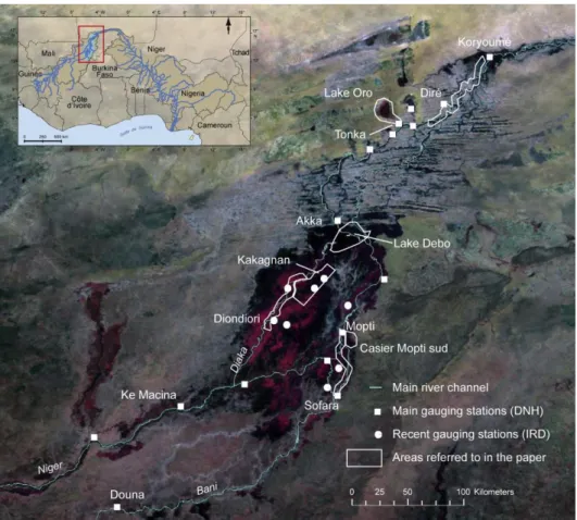
Fig. 1. Full colour composite MODIS image of the Niger Inner Delta with the principal sites mentioned in the paper.

Conversely, optical images are highly affected by cloud presence but are less sensitive to surface properties and are therefore suited to delineating water bodies in semi-arid areas with low annual cloud cover. However, opportunities provided by continued improvements in the spatial and temporal resolution of remote sensors and in image treatment and analysis must be further assessed and validated against field data.

The Inner Delta of the Niger River situated in central Mali, West Africa, is a large floodplain covering four million hectares and supporting over one million herders, fishermen and farmers (De Noray, 2003). Despite available global digital elevation mod- els (Shuttle Radar Topography Mission, Advanced Spaceborne Thermal Emission and Reflection Radiometer), and extensive field surveys carried out in the early 1980s, the knowledge about the floodplain topography remains insufficient to correctly model the propagation of the flood (Kuper et al., 2003; Neal et al., 2012). Detailed information on the spatial and temporal dynamic of the annual flood is of notable interest to stakeholders, consid- ering the established correlations between the flood levels and the associated ecosystem services, including fish, fodder and crop production (Liersch et al., 2013; Morand et al., 2012; Zwarts et al., 2005). Early attempts by Olivry (1995) estimated the vari- ations in the flooded surface areas through a water balance, exploiting the proportionality between flooded areas and total evaporation losses, but focussed on the Niger Inner Delta (NID)

as a single entity. Similarly, a Mike Basin model of the Niger River was developed by DHI but considered the delta as a single reservoir. Kuper et al. (2003) modelled the flood based upon 109 hydrological entities, using a simplified topography of the floodplain and river channels. The objective was to develop an integrated model of the wetland ecosystem services and explore management options with stakeholders but did not seek a physical representation of flood processes. To develop a finer and spatially explicit model of the delta, attempts have relied on agro-ecological models or remote sensing. Similarly to Cissé and Gosseye (1990), Marie (2000) attempted to use the fine knowledge of the vegetation dynamics in the southern part of the Inner Delta to develop a statistical relationship between the stage at Mopti and the types of vegetation flooded. Knowing the extent of each species over 22 000 km2 and which vegetation classes are flooded for each stage height, he estimated the corresponding flooded surface area. It could not take topographic effects into account, nor the delay between the flood in the upstream and downstream parts of the NID but provided an estimate of flooded surface areas as well as information on associated ecosystem dynamics. The Carima 1D model with flood storage cells (SOGREAH, 1985) represented flow down the main river channel and overflow into longitudinal plots, but lacked data to validate flood dynamics in the floodplain and operated at a low spatial resolution (20 km).

Recent studies using optical remote sensing on the NID pro- vided essential information on the scale of the flood but were lim- ited in the number of images used during the flood rise or decrease, notably due to image availability, cost and cloud cover. Zwarts et al. (2005) used Landsat images of 30 m resolution and an algo- rithm based on mid infrared reflectance to detect flooded areas. The method was developed on 24 images spanning 8 years of the late 1980s and the early 2000 to provide a spatially explicit model of the flooded areas for the varying dates and stage heights. Mariko (2003) used 1 km National Oceanic and Atmospheric Administra- tion Advanced Very High Resolution Radiometer (NOAA AVHRR) satellite images over 1990–2000 and employed a Full Colour Com- posite of Normalised Difference Vegetation Index (NDVI), brilliance index and a personal index based on near infrared to detect flooded areas. Seiler et al. (2009) later used the Gray Level Dependence Method (GLDM) on ENVISAT Advanced Synthetic Aperture Radar (ASAR) 30 m images combined with Normalised Difference Water Index (NDWI) on Advanced Spaceborne Thermal Emission and Reflection Radiometer (ASTER) images to study the flood over two dates.

Moderate Resolution Imaging Spectroradiometer (MODIS)

sensors, which gather daily images at 500 m resolution, open exciting prospects to follow the variations of the flood in wetlands with increased detail (Aires et al., 2014; Crétaux et al., 2011). However, are the quality, accuracy and resolution of remotely estimated flooded areas sufficient to correctly represent flood dynamics? At what temporal and spatial scales? How can the insights provided by this wealth of freely available spatial information be used in hydrology? The objective of this paper was to focus on these questions by developing a semi-automated method to monitor the progress of the flood in a large wetland exploiting large amounts of MODIS satellite images. The method was applied over a 11-year period in the Niger Inner Delta and confronted against extensive hydrological field data. Results are used to highlight how the increased temporal and spatial resolu- tion can improve the information available to stakeholders on the dynamics of the flood across the whole delta and in selected finer hydrological features. This knowledge is applied to refine the understanding of essential hydrological processes in the delta, notably evaporation and infiltration estimates and to provide 2D information on flood processes on which to build and calibrate future hydraulic models.

2. Study area and data 2.1. The Niger Inner Delta

The Niger River is the third longest watercourse in Africa after the Nile and Congo rivers. It is 4200 km long and flows northeast from the mountains in Guinea and Sierra Leone towards the vast floodplain of the Inner Delta and the Sahara, before heading South East towards Nigeria and the Gulf of Guinea in the Atlantic Ocean. Situated in Mali in West Africa (Fig. 1), the Niger Inner Delta, also known as the Inner Niger Delta or the Niger Inland Delta, is a 40 000 km2 _{floodplain, roughly 100 km wide and 400 km long.}

The NID is extremely flat, and the altitude of the river bed decreases by less than 10 m over the 400 km which separate the entry and exit of the delta. It is composed of a multitude of lakes, streams and marshes of varying morphology and two main parts can be distinguished: (1) the upstream delta from Ke Macina to Lake Debo, characterised by large independent channels in the dry season, which become totally flooded during the wet season and (2) the downstream delta from Lake Debo to Koryoumé com- posed of multiple small lakes and ponds separated by East–West oriented sand dunes (Brunet-Moret et al., 1986). Due to its

significant biodiversity, the Inner Delta is a wetland designated under the 1971 Ramsar Convention.

The Niger Inner Delta is situated in a semi-arid region where mean annual rainfall varies locally between 350 mm in the North and 700 mm in the South (Mahé et al., 2009), though this is subject to strong interannual variations. The River is therefore vital to the livelihoods of the riparian population, whose extensive agricultural practices evolved to harness the benefits of the flood. These consist primarily of fishing, floating rice (Oryza glaberrima), rainfed millet on the fringes of the flooded areas, as well as bourgou (Echinochloa stagnina) and other fodder for which livestock herders undertake large seasonal migrations (Ogilvie et al., 2010). Their production depends on the characteristics (timing, duration, depth, extent) of the annual flood highlighting the importance of assessing spatia- lised intra-annual and inter-annual variations in the flood dynamic. Hydrological extremes such as those caused by the drought in the 1980s notably led many perennial and temporary lakes to dry out, resulting in famine amongst riparian populations. The development of several dams and weirs upstream of the delta including Markala (in 1947), Sélingué (in 1981), Talo (in 2007), and potentially Djenné and Fomi, also affects the natural flow regime and reduces the amplitude of the annual flood (Marie, 2000; Zwarts et al., 2005).

The hydrological year for the Niger River and the Inner Delta is defined according to the regional unimodal rainfall pattern and runs from May to the following April. The rainy season peaks between the months of June and September, but because the flood is generated by rainfall 500 km upstream rather than locally, peak flow values occur between the months of September and Decem- ber due to propagation lag times.

2.2. Remote-sensing optical data

MODIS sensors, aboard the NASA Aqua and Terra satellites, pro- vide multispectral medium-resolution satellite imagery, suitable for studying large hydrological systems superior to 10 000 km2

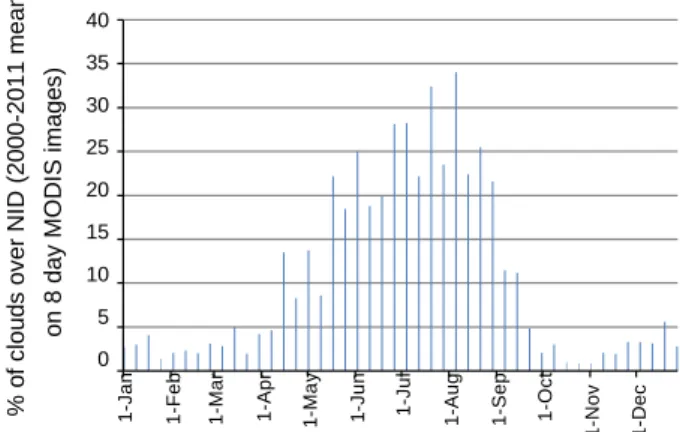
(Sakamoto et al., 2007). As moderate resolution sensors, they ben- efit from a large swath and shorter recurrence periods, allowing them to capture daily images. This temporal resolution is relevant for monitoring floods that have slow dynamics, such as the annual flooding controlled by the monsoon of the floodplain of the central Niger River and the lower Mekong River. Images are available since 2000 from the Terra satellite, while image acquisition for the Aqua satellite began two years later. The sensor acquires data at 500 m or higher spatial resolution from seven spectral bands (out of the 36 bands it detects) from the visible to the midinfrared spectrum, allowing the use of many classical composite band ratio indices. Though optical remote sensing is strongly affected by clouds and other atmospheric disturbances, which interfere with reflectance values, MODIS images can be used in the NID because most of the flood occurs when cloud cover is low. Indeed the flood is mainly caused by precipitation in the upper catchment and the flood peaks a few weeks after the rainy season.

The fifth version of the ‘‘MOD09A1’’ surface reflectance data set with an 8-day temporal resolution and a spatial resolution of approximately 500 m were used in this study. These 8-day com- posite images provided by NASA compile in one image the best sig- nal observed for each pixel over the following 8-day period and help reduce errors due to clouds, aerosols or viewing angle. The images provided include radiometric corrections notably against diffusion and absorption by atmospheric gases and aerosols and geometric corrections. These images limit the risk of prolonged periods without a suitable image for the whole area. On the down- side, the lag between two pixels can be anywhere between 1 and 15 days. MODIS images are freely distributed and rapidly available,

% o f c lou d s o v e r N ID (2000 -2 0 1 1 mea n o n 8 d a y MOD IS im a g e s ) 1 -Jan 1

-Feb ₁-Mar ₁-Apr

1

-M

a

y

1

-Jun 1-Jul ₁-Aug ₁-Sep ₁-Oct

1

-Nov

1

-Dec

and a single image covers the entire Inner Delta, avoiding the need for mosaicking pre-treatments.

Images were ordered via the Reverb interface from the Land Processes Distributed Active Archive Center (LP DAAC), which is a part of NASA’s Earth Observing System (EOS). A total of 526 images covering the period between July 2000 and December 2011 were downloaded and treated. The method was developed on images for the hydrologic year running from May 2001 to April 2002, and from May 2008 to April 2009. Subsets of about 800 km in longitude by 480 km in latitude centred on the NID were extracted in GeoTIFF file format from the MODIS HDR files and projected to the Universal Transverse Mercator (UTM) 30 North coordinate system using the MODIS Reprojection Tool Batch programme (Dwyer and Schmidt, 2006).

Four sets of images provided by the Enhanced Thematic Map- per+ sensor of the Landsat 7 satellite were also acquired for differ- ent phases of the 2001–2002 and 2008–2009 flood to calibrate and evaluate the method. These images possess a spatial resolution of 30 m and data from six spectral bands from the visible to the mid- infrared spectrum. Care was taken to select images with low cloud cover. Due to the higher spatial resolution, the coverage is lower, and two images were needed and mosaicked to cover the Inner Delta.

2.3. Hydro-meteorological data

The Niger River due to its regional and transboundary impor- tance benefits from a significant hydrological observation network, managed by Mali’s Direction Nationale de l’Hydraulique. There are 43 flow gauging stations in the Inner Delta with data ranging back to 1923, though time series are incomplete. As historical stations are principally located on the main stream channels, we installed in 2008 eight additional gauging stations (automatic pressure transducers and manually read vertical staff gauges) in the upstream part of the Inner Delta to record water stage on the Diaka tributary and in the floodplain. Stage data from irrigated rice plots around Mopti were also acquired from the Office du Riz Mopti (ORM). Furthermore, daily rainfall data from 5 gauges in the DIN over the period 2000–2009 were acquired through Mali’s Direction Nationale de la Météorologie. Field data were preferred over remo- tely acquired datasets such as Tropical Rainfall Measuring Mission (TRMM) considering their greater accuracy at this temporal and spatial scale. Nicholson et al. (2003) showed that the correlation between TRMM rainfall data and field data in West Africa was excellent at the seasonal scale for pixels of 2.5 spatial resolution. At the monthly, 1 scale needed for this study considering the spa- tial rainfall variability, the error was greater than 2 mm/day in August over half the grid cells tested, which corresponds to 40% of the mean August rainfall over 2000–2009. Monthly potential evapotranspiration (PET) values for 2008–2009 extracted from Cli- mate Research Unit (CRU) 0.5 spatial resolution products (Harris et al., 2014) as we only disposed of field data from two stations

(Mopti and Tombouctou). Satellite derived PET datasets

(Bastiaanssen et al., 1998; Weedon et al., 2011) were not used as they typically require additional meteorological data and provide greater benefits when studying actual evaporation over different land surfaces. The CRU PET values are calculated from half-degree values of mean temperature, maximum and minimum tempera- ture, vapour pressure and cloud cover and mean monthly wind val- ues. The FAO grass reference evapotranspiration equation (Ekström et al., 2007), a variant of the Penman Monteith formula is used. Associated uncertainties stem from the station data, the interpola- tion technique and the model used. When compared to available station data for Mopti and Tombouctou over 2008–2009, we found CRU PET values to be 12% lower in both cases.

40 35 30 25 20 15 10 5 0

Fig. 2. Mean cloud interference over the Niger Inner Delta on MODIS 8 day images over 2000–2011.

3. Method

The method relied on the assessment of flooded areas using a composite MNDWI and NDMI index on MODIS images, shown below to provide the best results out of 6 indices. Their perfor- mance and the optimal thresholds were assessed using confusion matrices against k-means classified Landsat images. An IDL pro- gramme combined areas detected by both indices for the 526 images over the period 2001–2011 and provided spatial and quan- titative assessments of the flooded areas for each 8 day MODIS image. Based on the analysis of cloud interference on MODIS images notably during the flood rise, time series of the flooded areas were smoothed. Results assessed the coherence of the remo- tely sensed flood dynamics across the wetland and within selected hydrological features such as lakes and floodplains, based on field instrumentation. Results were compared with previous studies and known correlations between Mopti stage data and flooded areas were refined to account for the varying amplitude of the flood and the hysteresis observed during the flood decline. Finally, wider applications in agricultural water management and hydrology namely to refine the water balance of the wetland were discussed and illustrated.

3.1. Detection of cloud interference

Though MODIS 8 day composite images (MOD09A1) seek to use the clearest pixel over an 8-day period, vapour clouds remained present in the downloaded images. As clouds reflect and absorb energy, their presence introduces errors in the reflectance values observed by satellite sensors, which can lead to difficulties and notably overestimation of flooded areas. Cloud information is con- tained in the Quality Assurance (QA) bits of MODIS scientific data sets (SDS). These SDS files are enclosed within the MODIS HDF files provided by NASA. A batch process of the MODIS Reprojection Tool (MRT) was used to first extract SDS files from the 526 HDF MODIS files, crop and reproject them to WGS 84 Universal Transverse Mercator 30 N. A second tool (Roy et al., 2002) provided by the Land Data Operational Products Evaluation (LDOPE) facility responsible for Quality Assurance issues relating to MODIS images, was used to extract and display the QA bits from MODIS scientific data sets (SDS), and allow detection and quantification of cloud presence. An IDL programme then computed for each image the percentage of cloudy and mixed (i.e. non-clear) pixels over the NID area and generated a corresponding Geotiff file locating the clouds.

The Geotiff images and statistical results on the percentage of cloudy pixels per image showed that clouds covered on average 10% of the NID area in the 2000–2011 MODIS images. Between

commission omission

C om m is s ion ra te C om m is s ion ra te C om m is s ion ra te Om is s ion ra te Om is s ion ra te Om is s ion ra te C om m is s ion ra te C om m is s ion ra te C om m is s ion ra te Om is s ion ra te Om is s ion ra te Om is s ion ra te 1.2 0 1.2 0 1 0.5 1 0.5 0.8 1 0.8 1 0.6 1.5 0.6 1.5 0.4 2 0.4 2 0.2 2.5 0.2 2.5 0 3 -1.0 -0.5 0.0 0.5 1.0 MDNWI value 0 3 -1.0 -0.5 0.0 0.5 1.0 NDMI value 1.2 1 0.8 0.6 0.4 0.2 0 0.5 1 1.5 2 2.5 1.2 1 0.8 0.6 0.4 0.2 0 0.5 1 1.5 2 2.5 0 -1.0 -0.5 0.0 0.5 1.0 3 0 -1.0 -0.5 0.0 0.5 1.0 3

NDVI value NDTI value

1.2 0 1.2 0 1 0.5 1 0.5 0.8 1 0.8 1 0.6 1.5 0.6 1.5 0.4 2 0.4 2 0.2 2.5 0.2 2.5 0 -1.0 -0.5 0.0 0.5 1.0 3 0 -1.0 -0.5 0.0 0.5 1.0 3

NDWI value NDPI value

Fig. 3. Confusion matrices between Landsat k-means classified images and 6 band ratio indices for varying threshold values.

26 and 35 images out of 46 images per year contained less than 10% clouds. Between September and April, cloud presence remained low (3.9% on average) but during the months of May– August (Fig. 2), the cloud presence rose considerably to 23% of the NID area, disturbing most years the monitoring of the rise of the flood. Excluding images with more than 10% or 15% clouds was seen to improve the coherence of the flood time series; however, to maintain sufficient images to follow the flood through all phases whilst reducing errors due to clouds, time ser- ies of flooded areas were smoothed using exploratory data

analysis methods (Tukey, 1977). Shown to be efficient in remov- ing outliers, these methods assume that time series vary smoothly over time and seek to remove the rough component, using repeated applications of a combination of running median smoothers on short subsequences and full sequences, and Han- ning linear smoothers. As a result of regular cloud presence dur- ing the flood rise, remotely sensed flooded areas for this phase may be overestimated. In 2001–2002 and 2008–2009 the reduced cloud presence allowed a more accurate detection of the flood rise.

þ

þ

þ

þ

þ 3.2. Discrimination of flooded areas in MODIS optical images

3.2.1. Remote sensing principles

The band ratio indices referred to in this paper are defined with MODIS spectral bands as

B2 B1 Remote sensing of water bodies relies on the principle that land

surfaces reflect energy differently according to their physical prop-

NDVI ¼

B2 B1 ð1Þ

erties. In optical remote sensing, the reflectance of water is com-

B4 B2 posed of its surface reflectance, volume reflectance and bottom

reflectance, though surface reflectance is the most significant

NDWI ¼

B4 B2 ð2Þ

(Mather, 1999) whatever the wavelength (Mobley, 1994). Shorter _{B4 B6}

wavelengths in the visible part of the electro-magnetic spectrum are highly reflected by the surface of water bodies, while longer

MNDWI ¼

B4 B6 ð3Þ

wavelengths, notably in the infrared are strongly absorbed. By con- _{B6 B4}

trast, soil and healthy vegetation strongly reflect energy in the near infrared (NIR) spectrum and vegetation has a low reflectance in the

NDPI ¼

B6 B4 ð4Þ

red spectrum. In addition reflectance in midinfrared (MIR) wave- _{B1 B4}

lengths is known to be sensitive to vegetation water content. As a result of these properties, reflectance values in the red, NIR and

NDTI ¼

B1 B4 ð5Þ

MIR spectra are particularly suited to distinguishing water bodies _{B2 B6}

from vegetation and bare soils (Annor et al., 2009; Liebe et al., 2005; Toya et al., 2002). Longer wavelengths (bands 5, 6 and 7 in

NDMI ¼

B2 B6 ð6Þ

MODIS) are also less perturbed by the reflectance generated by sed- iments and bottom reflectance in shallow waters (Li et al., 2003).

Variations in the reflectance values observed in specific spectral bands can therefore be used to distinguish types of land cover by thresholding reflectance values on a single band (here red, NIR or MIR) (Frazier and Page, 2000; Mialhe et al., 2008). A classical way to identify and delineate water bodies on multispectral satel- lite images is to define normalised band ratio indices using at least two bands. These improve detection accuracy as reflectance values are normalised across the image, reducing the influence of local- ised distortion effects. Likewise, normalised indices also reduce the effect of distorsions over consecutive images and allow the same threshold to be applied at several dates thereby facilitating automation of the procedure. Finally they are better than single bands at taking into account turbid water or submerged vegeta- tion, for which the reflectance profiles are less characteristic. A widely used index is the NDVI (cf. Eq. (1)) computed from the near infrared and red bands and proposed by Rouse et al. (1973) to detect vegetation in images. This index can be used to detect water pixels (Mohamed et al., 2004), where it takes on negative values. Several other indices exploiting the sharp contrast between the reflectance of water in the visible and infrared spectra have been proposed to detect water, notably the Normalised Difference Water Index (NDWI, cf. Eq. (2)), proposed by McFeeters (1996) and calcu- lated from the green and near infrared bands. To enhance the capacity of the NDWI to distinguish water pixels, Xu (2006) pro- posed the use of midinfrared instead of near infrared and called this new index the Modified Normalised Difference Water Index (MNDWI, cf. Eq. (3)). Lacaux et al. (2007) used the opposite of this index to identify temporal ponds in Senegal, and referred to it as the Normalised Difference Pond Index (NDPI, cf. Eq. (4)). These authors also used the Normalised Difference Turbidity Index (NDTI, cf. Eq. (5)) computed from the red and green bands, to measure the water turbidity in ponds in accordance with the Beer–Lambert law (Mobley, 1994). Another index using the near and mid-infrared spectral bands was proposed initially by Hardisky et al. (1983) under the name of Normalised Difference Infrared Index. It was

subsequently proposed by Xiao et al. (2005) under the name of Land Surface Water Index (LSWI) and confusingly by Gao (1996) under the name of NDWI and finally by Xu (2006) as the Norma- lised Difference Moisture Index (NDMI, cf. Eq. (6)). It was initially developed to detect the vegetation water content and by extension can be applied to detect partially submerged vegetation (Xiao et al., 2005). In order to discriminate all forms of water (open water, shallow waters, submerged vegetation), the strengths of each band and index can be combined (Crétaux et al., 2011).

þ where B1 contains reflectances from 620 nm to 670 nm (red), B2

from 841 nm to 876 nm (near infrared), B4 from 545 nm to 565 nm (green), and B6 from 1628 nm to 1652 nm (midinfrared). 3.2.2. Comparing and calibrating band ratio indices to detect flooded areas

An unsupervised classification in 15 classes was first performed on the six spectral bands of four Landsat images (October 2001, April 2002, October 2008 and April 2009) using the K-means clus- tering method. This iterative algorithm seeks to classify pixels into clusters and minimise the sum of the squared distance in the spec- tral space between each pixel and the assigned cluster centre. The 15 clusters were reduced to 4 classes (open water, submerged veg- etation, dry soils and dry vegetation) based on existing land use maps, knowledge of the area, and the spectral profiles of each clus- ter. Open water and submerged vegetation classes were then aggregated to ‘‘flooded areas’’, and dry soils and dry vegetation were grouped into ‘‘non-flooded areas’’ to produce a binary image. The unsupervised clustering approach, which provides excellent results (Jain, 2010), could be carried out on the four Landsat images but as it is nonparametric and image dependent, we required a fast, repeatable method based on objective parameters such as band ratio thresholds for the 526 MODIS images.

The six band ratio indices discussed in Section 3.2.1 (NDVI, NDWI, MNDWI, NDTI, NDMI, NDPI) were computed on MODIS images to compare their ability against concurrent classified Land- sat images to discriminate flooded areas when water levels were high (October) and low (April). A programme in the R language was used to calibrate the thresholds of the 6 band ratio indices by producing confusion matrices between each band ratio com- puted on MODIS images and two classified Landsat images for varying threshold values. The indices and associated thresholds which resulted in the lowest errors of omission and errors of com- mission were determined accordingly. The method’s consistency was assessed with confusion matrices against two additional clas- sified Landsat images.

3.2.3. Automated flood detection

A programme was written in the IDL _{language to automate the}

detection of flooded areas on the 526 MODIS images, chosen to monitor the annual and interannual variations of the flood. The IDL routine automatically computed the chosen composite MNDWI-NDMI index for each image and applied the thresholds previously determined to identify the flooded pixels. The IDL pro- gramme created GeoTIFF files of the flooded area for each image and compiled within a table the percentage of flooded pixels for

N ID e s ti mat e d f loo d e d a re a ( k m 2) N ID -MOD IS e s ti mat e d f loo d e d a re a ( k m 2) May -01 Nov -01 May -02 Nov -02 May -03 Nov -03 May -04 Nov -04 May -05 Nov -05 May -06 Nov -06 May -07 Nov -07 May -08 Nov -08 May -09 Nov -09 May -10 Nov -10 May -11 Nov -11 Mop ti s ta g e ( m a .s .l .)

Flooded area Flooded area (smooth) Stage

268 20000 267 16000 266 265 12000 264 8000 263 4000 262 261 0 260

Fig. 4. Flooded surface area in the Niger Inner Delta and Mopti stage values over the period 2000–2011.

25,000 23,000 21,000 19,000 17,000 15,000 13,000 11,000 9,000 7,000 5,000

MODIS 2000-2011 (this study) NOAA 1990-2000 (Mariko, 2003) Landsat 2000-2003 (Zwarts et al., 2005) MODIS 2000-2010 (Aires et al., 2014)

R2 = 0.93

around 1000 pixels (i.e. around 200 km2_{) were delineated centred}

on hydrological features (Fig. 1). The programme accepted cells issued from a meshing software (such as SMS ems-i) or in shape- file format, and calculated the number of flooded pixels over time in each hydrological feature. Correlations between remotely sensed flooded areas and corresponding field data were then stud- ied to confirm the coherence of remotely sensed flood dynamics within hydrological units. These focussed on 2008–2009, when the largest sets of hydrological and remote sensing data were avail- able. Gauging stations were available at the upstream and down- stream end of selected features but as the flood dynamic was homogeneous across each hydrological unit, the gauge with the most complete time series was used in the analysis.

1500 1700 1900 2100 2300 2500 2700 2900 Mopti - October mean monthly flow (m3/s)

Fig. 5. Relationship between Mopti maximum monthly flows (October) and peak flooded areas.

each 8 day period. A mask was applied to exclude pixels which are not part of the NID, in order to increase processing speed. 3.3. Comparing remotely sensed flood dynamics with hydrological field data

Remotely sensed areas for the whole wetland over an 11 year period were compared with previous estimates and with existing correlations with field stage data (Aires et al., 2014; Mahé et al., 2011; Zwarts et al., 2005). Interannual variations in the timing, magnitude and duration of the flood and their consistency with hydrological observations were then explored.

A grid based on the hydrological features present in the NID developed for a previous model of the wetland (SOGREAH, 1985) was also adapted to study flood dynamics in selected hydrological units. Units were chosen to highlight the heterogeneous flood pro- cesses across the range of hydrological features present in the wet- land, i.e. river channel, floodplain, lake and irrigated area, and according to the location of installed hydrological field equipment.

To smooth out individual spurious pixels resulting from incorrectly classified binary pixels, large cells aggregating information from

3.4. Water balance of the wetland

500 m resolution assessments of the flooded surface area at an 8-day timestep provided by MODIS images were used to assess rainfall and evaporation over the wetland, and refine its water bal- ance. Daily time series from Ke Macina situated upstream on the Niger river were combined with those from Douna gauging station on the Bani tributary to assess inflows into the wetland. Due to the construction of the Talo dam on the Bani river in 2005, subsequent time series at Douna were interpolated from downstream and upstream data. Outflow from the wetland was estimated at the Koryoumé gauging station downstream. Climatic variables (monthly 0.5 PET and daily rainfall values) were interpolated spa- tially over the wetland using Thiessen polygons and converted to the MODIS 8-day timestep. These values were multiplied by the corresponding MODIS estimated flooded area to assess actual evaporation from the wetland and direct precipitation into the wetland. The water budget residual term was then the difference between infiltration from the flooded areas and effective precipita- tion over nonflooded areas.

For 2008–2009, daily rainfall values were first interpolated over three subsections (based on isohyets) and monthly spatially expli- cit PET values for 140 cells (Fig. 15) were used. These results were compared with results obtained using daily P and monthly PET val- ues interpolated across the whole wetland, which showed that total P and PET from the wetland varied by less than 10%. As a result, calculations for the 11 year period used values of P and

N ID M OD IS e s ti mat e d f loo d e d a re a ( k m 2) 20,000 18,000 16,000 14,000 12,000 10,000 8,000 6,000 4,000 2,000 2001-02 decline 2004-05 decline 2005-06 decline 2008-09 decline 2001-02 rise 2004-05 rise 2005-06 rise 2008-09 rise 261 262 263 264 265 266 267 268

Mopti - stage (m a.s.l.)

Fig. 6. Relationship between the 8 day stage value at Mopti and corresponding flooded area across the NID as the flood rises and recedes for 4 floods of varying amplitude.

PET interpolated across the whole wetland. Sensitivity of the water balance to uncertainties was estimated.

4. Results and discussion

4.1. Ability of band ratio indices to discriminate flooded areas Confusion matrices were used to compute pixel classification accuracy between the thresholded band ratio MODIS images and the k-means classified Landsat images. The lowest errors of omis- sion and errors of commission were obtained using the MNDWI, NDMI and NDVI indices (Fig. 3). MODIS classified images showed that the NDVI detected vegetation correctly in the NID but was less suited to distinguish between soils and pure water and between dry and flooded vegetation. The MNDWI was most suited to the detection of all types of water. It identified the water bodies and certain parts of flooded vegetation and could be used alone during periods of deep water. However, as the flood recedes and the areas of flooded vegetation become proportionally more important, the vegetation growth led to difficulties in water detection, and the MNDWI systematically under-estimated water surfaces. The Inner Delta notably supports large areas of Bourgou (Echinochloa stagnin- a) which thrives in water depths up to 4 m and can be submerged during 6 months. The NDMI, which was capable of identifying sub- merged vegetation but failed to reliably detect pure water was therefore chosen to complement the MNDWI. NDTI identified flooded vegetation correctly but was less discriminant between clear water and bare soils. NDWI was proficient in identifying pure water and parts of the flooded vegetation. Values for these land uses were also respectively high and very low, hence no single threshold could be used.

For the MDNWI, classifying pixels above the threshold of 0.34 as flooded areas produced the nearest match with the classified Landsat image during high floods (October 2001, 86% of well clas- sified pixels) and during low floods (April 2002, 88% of well classi- fied pixels). Incorrectly classified pixels can be explained by the inherent uncertainties (atmospheric, radiometric) in the measure- ment of spectral reflectances and in the classification of flooded vegetation and shallow waters. The variation in the flooded surface area detected by using a threshold of 0.3 and 0.4 was significa- tive: during the flood, the difference was about 4% but in the dry

period it reached 23%. The second decimal in the threshold thus needed to be taken into account, contrarily to what was done in Sakamoto et al. (2007). For the NDMI, pixels above the threshold value of 0.15 were considered. The areas detected by the two thres- holded indices were then added, i.e. an area that met either condi- tion was identified as flooded, effectively creating a composite index.

Confusion matrices between MODIS images and two additional Landsat k-means classified images (October 2008 and April 2009) showed that 85% of pixels were correctly classified. The result, comparable to 87% of correctly classified pixels on the 2001– 2002 images, confirmed the method’s consistency in detecting flooded areas, compared to Landsat classifications.

4.2. Flood monitoring at the Inner Delta level

4.2.1. Annual and interannual flood dynamics (2000–2011)

This method, which allows the automated treatment of vast quantity of images, was applied to 526 MODIS images of the NID covering the period between July 2000 and December 2011. Over the 11 hydrological years studied, the peak flooded surface area varied between a maximum flood of 20 000 km2 _{in autumn 2008}

and a minimum of 10 300 km2 _{in autumn 2011. The 2000–2011}

mean of the maximum flooded surface area was 16 000 km2 _and

the standard deviation 3400 km2_{, providing insight into the signif-}

icant interannual variability in the extent of the flood.

During the dry season, the flooded surface area receded pro- gressively to a minimum of 3800 km2 _{(2000–2011 interannual}

mean) the following April before increasing during the month of June and rising rapidly in August. Minimum values, measured between mid March and mid April using images with less than 10% clouds, varied between 3000 km2 _{and 4000 km}2_{. Images for}

the later months were heavily influenced by cloud presence and could not be reliably used. Furthermore, when water levels are low and vegetation becomes important, the signal and therefore boundaries of water, soil and vegetation are noticeably hard to dif- ferentiate (Mialhe et al., 2008). No correlation between the peak and minimum flooded areas over a hydrological year was found, despite the former influencing the amount of water trapped in lakes and depressions, partly due to difficulties in estimating

20000 2001-02 2002-03 2004-05 2005-06 2008-09 Peak flood (2000-2010) 2001-02 2002-03 2004-05 2005-06 2008-09 Peak flood (2000-2010) 15000 N ID - M OD IS e s ti m a te d f loo d e d area ( k m 2) 25000 10000 5000 0 260 261 262 263 264 265 266 267 268 Mopti - stage (m a.s.l.)

Fig. 7. Relationship between 8 day stage values at Mopti and total flooded areas as the flood declines according to the amplitude of the flood peak in October. 5 floods of varying amplitude are represented.

flooded areas during the dry season, and exceptional rainfall in March–April.

The Mopti gauging station is regularly used to model the annual floods in the Delta (Mahé et al., 2011; Zwarts et al., 2005), due to its central location where it perceives flow variations in the Niger river and indirectly the Bani river, a major tributary. Fluctuations in the total flooded area are indeed known to be driven by changes in rainfall of the Niger and Bani upper catchments (Mahé et al., 2009). The annual flood dynamic observed through remote sensing appeared coherent with Mopti flow regime (Fig. 4), providing con- firmation of the method’s ability to correctly represent the phase of the flood. Interannual variations in the peak flooded areas were also strongly correlated (R2 = 0.93) with the peak monthly flows in October at Mopti confirming the method’s capacity to represent the variations in the peak amplitude of the flood (Fig. 5). Peak val- ues were obtained using the maximum value for images between 8 October and 9 November, and manually excluding inconsistent peak values. This appeared legitimate, considering the prolonged peak flood. The range of values obtained and their variation accord- ing to peak flow in October (Fig. 5) were consistent with previous remotely sensed estimates (Aires et al., 2014; Mariko, 2003; Zwarts et al., 2005), though values were moderately superior. The differ- ence in absolute values reveals the difficulty in assessing flooded surface areas accurately and may be due to better detection of flooded vegetation areas, with the NDMI, as well as differences in the delimitation of the wetland boundaries. Furthermore Zwarts et al. (2005) could not monitor directly the flood progress over a year, but instead relied on a correlation between 24 Landsat images spread over several years to derive a correlation between flooded areas and the Akka stage level. Mariko (2003), who used NOAA AVHRR products, was limited by the number of suitable images, due to the presence of clouds and geometric distorsions. 4.2.2. Stage–surface area correlations accounting for hysteresis and amplitude

The relationship between stage values at Mopti and the concur- rent flooded surface area across the whole NID was also explored for each image over the 11 years. To account for the fact that MOD09A1 images are a composition of pixels over the following 8 days, the corresponding average 8 day stage at Mopti was used. The flood rise (August–October) and decline (November–April) were differentiated in order to isolate the hysteresis behaviour described in Section 4.2.3, which causes flooded areas to recede

much more gradually than they increase during the flood rise. The difference in the stage–surface area for both phases of the flood is shown in Fig. 6, which also illustrated how the relationship varies according to the amplitude of the flood. As the flood recedes, the flooded surface area is indeed determined by the amount of outerlying disconnected areas which were flooded during the flood peak. Accordingly, the hysteresis seen in Fig. 6 was most significant for the largest floods. Previous research suggested this (Mahé et al., 2011; Zwarts et al., 2005), but could not examine this due to an insufficient amount of images per year. During the flood rise (Fig. 6) the stage–surface area relationship is also indirectly deter- mined by the amplitude of the peak flood. Indeed depending on the amplitude, when stage reaches a certain value at Mopti, a larger flood wave will have flooded larger areas upstream of Mopti in a stronger year. Analysis was however limited by the cloud interfer- ence during the flood rise which may have overestimated flooded areas.

Due to the regional importance of the flood in the Inner Delta, these relations are of interest to stakeholders, and have in the past been linked through simple regression models to variations in upstream river levels (Mahé et al., 2011; Zwarts et al., 2005). Zwarts (2010) notably estimated from August flow data, the November stage levels at Mopti and Akka and the corresponding estimated flooded area. Our correlations improve upon former sta- tistical relationships by distinguishing the amplitude of the peak flood and increasing the accuracy of estimated surface areas. Fig. 7 can be used to provide from the peak flow value in October an estimate of the peak flooded area across the whole wetland and an estimation of the flooded areas as it recedes. Care must be taken when extrapolating this relationship for floods beyond the range studied here, i.e. peak floods between 10 000 km2 _and

20 000 km2_{. Furthermore, simulations of past or future floods must}

also account for possible changes in the NID hydraulic pathways due to dams or land use changes.

4.2.3. Spatial heterogeneity of the annual flood

The treated MODIS images allowed the representation and spa- tial analysis of the annual flood’s progress through the NID (Fig. 8) at high spatial (500 m) and temporal (8 days) resolutions. The sig- nificant presence of clouds between May and August (Fig. 2) pre- vented an accurate monitoring of the arrival of the flood, except in 2008 as a result of limited cloud cover. The flood peak and sub- sequent decrease were consistently detected every year. These

Fig. 8. Monthly progression of the flood in the Niger Inner Delta over the 2008–2009 hydrological year.

images were then aggregated to compute a map of the duration each pixel remains flooded between August and the following April (Fig. 9). Combined with numerical estimates of flooded areas in selected hydrological units (Fig. 10), these maps revealed signifi- cant spatial specificities in the flood dynamic. These occur as a result of the time needed for the flood wave to travel downstream and of the geomorphological differences encountered as the flood extends laterally. The hysteresis like behaviour which occurs when water remains trapped in lakes and agricultural plots, naturally by the riverbanks or intentionally through a system of manually oper- ated gates, leads to significantly delayed and prolonged floods. The greater presence of lakes and depressions in the North of the wet- land explains the longer flooding in this area (Mahé et al., 2009), which in 2008–2009 lasted principally between September and January, with a peak delayed until late November. In the South the flood receded much faster lasting between the months of August and November, with a peak flood occurring in early Octo- ber. This marked delay is in line with former observations (Brunet-Moret et al., 1986) and concurs with available flow data in the main river channels.

Fig. 8 showed that the flood in the South had in fact nearly sub- sided from evaporation and flow downstream, when the North

became flooded. Conversely, Lake Oro in the North was still emp- tying when the upstream part begun to flood again (Fig. 10a and d). These spatial differences in the timing and duration of the flood must be accounted for when modelling the propagation of the flood within the delta, and the NID cannot be represented as a sin- gle unit or reservoir with a homogenous and gradual flood dynamic. Visualising the parts of the wetland flooded during the high flood in 2008–2009 (Fig. 9) could also lead to defining the contours of a suitable modelling grid, though a margin for the expanse of the flood in exceptional years must be included. The spatial heterogeneity observed in the flood duration and timing could also be used to derive a typology of flood dynamics and help define how cells can be aggregated and the corresponding optimal spatial resolution of the model.

4.3. Flood monitoring at the hydrological unit level

The percentage of flooded pixels calculated for each MODIS image in selected hydrological features (Fig. 1) was compared with corresponding available stage data. In cells along the main riverbed such as Mopti, Ke Macina and Diré (Fig. 10a), the flooded areas rose and receded in accordance with the relatively sharp and short flood

D iré ri v e r c ha nnel M O D IS e s ti m at e d flood ed area ( k m 2) M op ti-Su d T ib o ric e pl ot s tage (m a .s .l .) May -08 6 -Aug 20 -Aug Aug -08 3 -Sep Nov -08 17 -Sep Feb -09 1 -Oct May -09 15 -Oct 29 -Oct Aug -09 12 -Nov Nov -09 26 -Nov Feb -10 10 -Dec 24 -Dec May -10 7 -Jan D iré s tage (m a. s .l) Lak e O ro M O D IS e s ti m a ted f lood e d ar ea (k m 2) D ion diori f lo odpl ain M O D IS e s ti m a ted flood ed area (k m 2) May -08 May -08 Aug -08 Aug -08 Nov -08 Nov -08 Feb -09 Feb -09 May -09 May -09 Aug -09 Aug -09 Nov -09 Nov -09 Feb -10 Feb -10 May -10 May -10 D ion ddior i s tage ( c m ) T on k a s tage ( m a. s .l)

Fig. 9. Duration of the flood in the Niger Inner Delta between August 2008 and April 2009.

(a) (b) 500 450 400 350 300 250 200 150 100 50 0 (MODIS) Stage 262 261 260 259 258 257 256 350 300 250 200 150 100 50 0 Flooded area (MODIS) Stage 500 450 400 350 300 250 200 150 100 50 0 (c) (d) 267 266 265 264 263

MODIS estimated stage Diaby stage 250 200 150 100 50 0 Flooded area (MODIS) Stage 263 262 261 260 259 258 257 256

Fig. 10. Comparison between stage levels measured in situ and remotely sensed flooded surface areas for (clockwise from top left): (a) Diré, main river channel, (b) Diondiori, floodplain, (c) Mopti irrigated rice plot (Casier Mopti Sud Tibo) and (d) Lake Oro, situated on Fig. 1.

250 _{highlighted in Fig. 11b led to a greater surface area during flood} decline than flood rise for the same stage level at Diondiori. In Lake

Flood decline _{Oro (Fig. 10d), the flooded area also only begins to rise when river}

150 stage values reach a certain level (Batti, 2001). The connection

between the river, where the Tonka gauging station is situated,

100 _{and Lake Oro is however also influenced by a flood gate opened}

between October and February. Once river levels have risen suffi- 50

ciently and the gate is opened, flooded areas increase rapidly. In 0

0 100 200 300 400 500 600

February, when the lake has filled up, stage value has reduced and the gate has been closed, the lake becomes disconnected again

Diondior i stage (cm) from the river and water levels in the lake reduce from evapora-

Mop ti ri v e r c h a n n e l - MOD IS e s tim a te d floo d e d a re a ( k m 2) N ID a rea f loode d (k m 2) for x day s D ion d ior i floo d p lain MOD IS e s tim a te d floo d e d a re a ( k m 2) N ID a rea f loode d (k m 2) for at leas t x da y s 350 300 250 200 150 100 50 0

(a)

R2 = 0.91

hydrographs for nearby gauging stations. The high level of correla- tion is coherent with a geometrical stage–surface relationship, and provided partial confirmation of the ability to use MODIS images to study flood dynamics locally. Where correlations were good, the equations derived from these relations may be used to monitor water depths using daily or weekly MODIS images. Fig. 11a shows that the correlation remained stable over the 11 years, implying that these relations could assist in filling gaps in data series or extrapolating to years before equipment was in place. Conversely, past and future stage time series could be used to estimate the flooded surface area in these cells.

In floodplains (Fig. 10b), the flood dynamic observed remotely was slightly different to nearby stage measurements, but coherent 260 262 264 266 268

Mopti stage (m a.s.l.)

350

(b)

300

Flood rise

with geomorphological considerations. The flood rise was delayed due to the lag before the water in the riverbed overflows its bank and enters the floodplain. Likewise, as the flood recedes, a hyster- esis phenomenon leads to a slower decrease in flooded areas than stage, due to water remaining trapped in outer lying floodplains, which gradually dry out through evaporation, infiltration and water use. This different behaviour as the flood rises and recedes

200

Fig. 11. Correlations between stage levels measured in situ and remotely sensed flooded surface area for (a) Mopti, main river channel over 2000–2010 and (b) Diondiori, floodplain 2008–2009.

tion, infiltration and water use. Flood gates are reopened the fol- lowing October.

In irrigated rice plots topographic information enabled the pro- duction of a surface–stage relationship to convert MODIS esti- mated surface areas to estimated stage values. These showed a

3000 2500 2000 1500 1000 500 Area flooded x days Area flooded at least x days 35000 30000 25000 20000 15000 10000 5000

very similar trend to stage measurements available at the entrance of the canal at Diaby (upstream of the casier Mopti Sud), confirm- ing the accuracy of this method. Estimated stage values for the plots remained marginally lower which is coherent with the con- figuration, considering the natural slope present to convey water to the plots. Fig. 10c shows the plots filling in October and the gradual decrease from evapotranspiration and infiltration during rice growth until the end of November, when the sluice gates are opened. Results also reveal the rapid decrease in flooded area after

0 0 5 35 65 95 125 155 185 215 245 275

Number of days

Fig. 12. Surface area flooded according to the number of days in 2008–2009.

ceased. These examples illustrated insights which cannot always be inferred from nearby stage measurements and the ability of MODIS images to be used for relatively small areas (60 km2_{) and}

2001-2002 2002-2003-2004 2004-2005-2006 2006-2007-2008 2008-2009-2010 2010-2011-2012 K a k a g n a n f loo d p lain f loo d e d a re a ( k m 2) 500 450 2003 400 2005 350 2007 300 250 2009 200 2011 150 100 50 0 0 50 100 150 200 250 Number of days

Fig. 14. Flood duration curves for 2001–2011 in the Kakagnan floodplain of the Niger Inner Delta.

Fig. 15. Potential evapotranspiration and actual evaporation values from NID flooded areas in 2008–2009.

4.4. Understanding local flood dynamics in agricultural water management

The differences observed in local flood dynamics also have strong applications in agricultural water management, where understanding the timing and duration of the flood can help target and time irrigation practices (Fig. 9). In Lake Oro, for instance, the maximum surface area was reached in January, over one month later than in the nearby river channel, and remained flooded until the following September, providing a valuable resource during the dry season (Fig. 10d). To identify the total surface area in the NID available to support certain ecosystem services or crop cycles, based on the length of their irrigation requirements, flood duration curves at the NID scale were extracted from the spatial informa- tion. Fig. 12 shows that in 2008–2009 around 20 000 km2 were

flooded for at least 90 days, defining the areas where plots (with one to two metres water depth) are suitable for floating rice pro- duction (Liersch et al., 2013). Around 500 km2 _{remained flooded}

throughout the flood, mostly the main river channel and certain lakes, while the majority of the DIN remained flooded between 11 and 15 weeks. Large areas were flooded very briefly, notably the banks of rivers and lakes, as well as minor depressions filled by rainfall or the flood. The total (non synchroneous) flooded area during the August 2008 – April 2009 flood reached 32 550 km2_{, i.e.}

a total of 32 550 km2 _{were flooded at some time in the year, but}

only 20 000 km2 _{were flooded at the same time.}

Reduced floods, observed in 2002, 2004, 2005 and 2011, are known to have devastating consequences on the ecosystem ser- vices dependant on the flood, notably reduced rice production and fish production (Morand et al., 2012). Fig. 13 highlights how

N ID D a ily E ( k m 3) N ID A n n u a l flu x e s ( k m 3) M a y -0 8 Ju l-08 S e p -0 8 Nov -08 Ja n -09 M a r-09 M a y -0 9 N ID C u mula ti v e E (k m 3) 0.12 0.10 0.08 0.06 0.04 0.02 0.00 25 20 15 10 5 0

Fig. 16. Evaporation over the NID wetland in 2008–2009.

of evaporation losses across the NID (Fig. 15). PET values range from north to south between 2120 mm and 1650 mm, and mean PET across the NID is estimated at 1970 mm. This is marginally lower than previous estimates by Olivry (1995) of 2300 mm, and can be explained by the 12% lower CRU PET values compared to Mopti and Tombouctou station data as well as minor interannual differences.

Actual evaporation rates from the wetland varied between 4 mm/day and 7 mm/day over the year 2008–2009, which com- pare well with values between 3 mm/day and 7 mm/day in Dadson et al., (2010). In 2008–2009, cumulative evaporation losses from the whole wetland reached approximately 20 km3 _{(Fig. 16).}

This equates to 440 mm from the wetland or 1.2 mm/day, which is within the range of values modelled by recent studies over the same period, notably 1.1 mm/day (Dadson et al., 2010) and 1.8 mm/day (Pedinotti et al., 2012). In this study, evapotranspira- tion from non-flooded areas of the wetland (soil moisture, vegeta- tion) was not assessed, which would increase overall evaporation

Evaporation Inflow - Outflow Residual losses. However, evaporation from flooded areas may have been

overestimated slightly, as evaporation rates from wetlands (i.e.

Evaporation 30 25 20 15 10 5 0

Inflow - Outflow Residual

R2 = 0.91

R2= 0.94

R2 = 0.68

water bodies covered by vegetation) can be inferior to those of open water (McMahon et al., 2013). Uncertainties on remotely sensed flooded areas are however expected to be more determinant.

Though evaporation per flooded area was highest during the months of the dry season, total evaporation from the NID was superior during the months of October and November, due to the large surface area flooded. Likewise, spatial variations in actual evaporation (Fig. 15) were significant due to higher PET values in the Northern parts and the longer flood durations along river stretches and lakes. Over 2001–2011, annual evaporation varied between 12 km3 _{and 21 km}3 _{(Fig. 17) with a mean value of} 10000 12000 14000 16000 18000 20000

-5

22000 _{17.2 km}3_.

NID - flooded area (km2₎

Fig. 17. Correlation between water balance terms and the annual peak flooded area over 2001–2010.

the hydrological response in specific areas was more or less affected by the variations in the amplitude of the flood, due to the morphology of the different sections, with more shallow areas of the delta flooding more easily. Fig. 14 displays flood duration curves created from flood hydrographs for a floodplain. The flood across the hydrological unit was considered synchrone, consider- ing that these were delimitated on the basis of their homogeneous flood behaviour, i.e. areas where the timing, amplitude and dura- tion of the flood are similar. In 2004, when the peak flooded area in the NID was 45% lower than in 2008, the peak flooded area in this Kakagnan floodplain reduced by only 22% compared to 2008 (Fig. 14). Fish catch, directly correlated to the peak flooded area, also decreased by around 22% or 520 tonnes, based on a fish catch of 55 kg/ha (Morand et al., 2012). Areas flooded more than 90 days potentially suited to floating rice production however reduced by 33%, and possibly more as the crop requires a minimal water depth of one metre. The remote assessment of the flood dynamic within individual lakes and floodplains of the wetland thus provides increased opportunities for stakeholders to observe the impact of hydrological changes on dependent agricultural practices. 4.5. Improving the water balance of the NID

4.5.1. Spatial and interannual evaporation variations

Evaporation losses for 2008–2009 were calculated from MODIS estimated flooded areas and CRU PET data for 140 grid cells adapted from an existing grid (SOGREAH, 1985) providing a map

4.5.2. Accounting for rainfall and estimating infiltration

The difference between inflows to the wetland calculated from gauging stations on the Niger and Bani rivers and outflows at Kor- youmé ranged between 9.5 km3_{/year and 19 km}3_{/year over 2001–}

2010. This corresponds to a reduction ranging between 33% and 40% of annual inflows as water flows through the delta in line with previous findings (Mahé et al., 2009). The annual losses were strongly correlated with peak flooded areas (Fig. 17), confirming the hypothesis used in previous works to assess flooded areas from downstream losses (Mahé et al., 2009; Olivry, 1995).

Evaporation losses (Fig. 17) calculated using MODIS remotely sensed flooded areas were superior to the difference between inflow and outflow, highlighting the other fluxes which must be accounted for, notably the nonnegligible contribution of rainfall into the NID. Rainfall interpolated over the NID varied between 280 mm/year and 560 mm/year over 2001–2010, i.e. 33–66 km3_{/year over the total NID area. However, in the water balance,}

only effective precipitation must be accounted for. This is composed of direct rainfall falling on flooded areas (where the runoff coefficient is 1) and effective precipitation over nonflooded areas. Direct precipitation over the wetland calculated from interpolated rainfall over the MODIS flooded areas varied between 2.6 km3_{/year and 8.5 km}3_/year.

The water budget residual term is then the difference between infiltration over the wetland and runoff generated by rainfall fall- ing upon nonflooded areas of the NID. Interannual storage changes and flows from groundwater were neglected in line with previous studies (Mahé et al., 2002, 2009; Olivry, 1995), considering their minimal contribution. The calculated residual term of the water budget varied between 0.7 and 5 km3_{/year. Fig. 17 shows how}

for larger floods the residual is positive implying infiltration is superior to effective precipitation over nonflooded areas. This is