Nightside studies of coherent HF Radar spectral width behaviour

HAL Id: hal-00317140

https://hal.archives-ouvertes.fr/hal-00317140

Submitted on 1 Jan 2002

HAL is a multi-disciplinary open access

archive for the deposit and dissemination of

sci-entific research documents, whether they are

pub-lished or not. The documents may come from

teaching and research institutions in France or

abroad, or from public or private research centers.

L’archive ouverte pluridisciplinaire HAL, est

destinée au dépôt et à la diffusion de documents

scientifiques de niveau recherche, publiés ou non,

émanant des établissements d’enseignement et de

recherche français ou étrangers, des laboratoires

publics ou privés.

behaviour

E. E. Woodfield, J. A. Davies, M. Lester, T. K. Yeoman, P. Eglitis, M.

Lockwood

To cite this version:

E. E. Woodfield, J. A. Davies, M. Lester, T. K. Yeoman, P. Eglitis, et al.. Nightside studies of coherent

HF Radar spectral width behaviour. Annales Geophysicae, European Geosciences Union, 2002, 20

(9), pp.1399-1413. �hal-00317140�

Annales

Geophysicae

Nightside studies of coherent HF Radar spectral width behaviour

1_{Department of Physics and Astronomy, University of Leicester, UK}

2_{Formerly at Swedish Institute of Space Physics, Uppsala, Sweden and the Finnish Meteorological Institute, Helsinki, Finland} 3_{Rutherford Appleton Laboratory, UK}

4_{now at: Rhea System S.A., New Tech Center, Belgium}

5_{also at: Department of Physics and Astronomy, University of Southampton, UK}

Received: 17 October 2001 – Revised: 30 April 2002 – Accepted: 15 May 2002

Abstract. A previous case study found a relationship be-tween high spectral width measured by the CUTLASS Fin-land HF radar and elevated electron temperatures observed by the EISCAT and ESR incoherent scatter radars in the post-midnight sector of magnetic local time. This paper expands that work by briefly re-examining that interval and looking in depth at two further case studies. In all three cases a re-gion of high HF spectral width (> 200 ms−1) exists poleward of a region of low HF spectral width (< 200 ms−1). Each case, however, occurs under quite different geomagnetic con-ditions. The original case study occurred during an interval with no observed electrojet activity, the second study dur-ing a transition from quiet to active conditions with a clear band of ion frictional heating indicating the location of the flow reversal boundary, and the third during an isolated sub-storm. These case studies indicate that the relationship be-tween elevated electron temperature and high HF radar spec-tral width appears on closed field lines after 03:00 magnetic local time (MLT) on the nightside. It is not clear whether the same relationship would hold on open field lines, since our analysis of this relationship is restricted in latitude. We find two important properties of high spectral width data on the nightside. Firstly the high spectral width values occur on both open and closed field lines, and secondly that the power spectra which exhibit high widths are both single-peak and multiple-peak. In general the regions of high spectral width (> 200 ms−1) have more multiple-peak spectra than the re-gions of low spectral widths whilst still maintaining a ma-jority of single-peak spectra. We also find that the region of ion frictional heating is collocated with many multiple-peak HF spectra. Several mechanisms for the generation of high spectral width have been proposed which would pro-duce multiple-peak spectra, these are discussed in relation to the data presented here. Since the regions of high spectral width are observed both on closed and open field lines the use of the boundary between low and high spectral width as

Correspondence to: E. E. Woodfield

(Emma.Woodfield@ion.le.ac.uk)

an ionospheric proxy for the open/closed field line boundary is not a simple matter, if indeed it is possible at all.

Key words. Ionosphere (auroral ionosphere; ionospheric ir-regularities)

1 Introduction

The Doppler spectral width parameter observed by coher-ent HF radars is associated with the turbulcoher-ent characteristics of the plasma irregularities being illuminated by the radar. If one thinks of the spectral width (defined here as the full width at half maximum) in terms of the power spectrum it describes, then it is essentially a measure of how variable the Doppler line-of-sight velocity has been during the integra-tion period and within the spatial range of the radar obser-vation cell. However, the power spectra returned from the radar sometimes contain two or more separate and well de-fined peaks at different velocities. Under these circumstances the standard spectral width parameter does not tell the whole story and the spectra themselves require inspection. For some time now, the spectral width parameter observed by the Super Dual Auroral Radar Network (SuperDARN) coherent HF radars (Greenwald et al., 1995), has been used as an iono-spheric proxy for the position of the low-altitude cusp on the dayside. It is thought that within the cusp region the spectral width is high (> 150 ms−1_{) and variable (Baker et al., 1990,}

1995; Pinnock et al., 1995, Andr´e et al., 1999, 2000a; Mi-lan et al., 1999; Moen et al., 2001; Rodger, 2000; MiMi-lan and Lester, 2001; Pinnock and Rodger, 2001), although this is not always the case (Rodger et al., 1995). This feature is believed to be the result of the problems that the standard parame-ter fitting software (FITACF) (Villain et al., 1987) has fitting auto-correlation functions (ACFs) which lead to power spec-tra that have several large peaks. Hence the specspec-tral width and line-of-sight velocity are both more variable where the spectra have multiple-peaks, and the errors associated with the fitting of these parameters are increased (e.g. Andr´e et

al., 2000a). The low-latitude boundary layer (LLBL) has been associated with double-peak spectra from the Super-DARN radars (Schiffler et al., 1997; Huber and Sofko, 2000) and multiple-peak spectra (Baker et al., 1995). Regions of ionospheric backscatter with similar spectral width features to those seen in the cusp are also found frequently on the nightside (Lewis et al., 1997; Dudeney et al., 1998; Lester et al., 2001; Woodfield et al., 2002).

Several suggestions for mechanisms responsible for these multiple-peak spectra have been made. Looking at the cusp spectra, Andr´e et al. (1999, 2000a), have simulated high spectral widths in the radar data by the use of a time-varying electric field with a frequency in the Pc1/Pc2 band (0.1 to 5 Hz). The occurrence of such waves is observed to increase in a step-like manner when low-altitude satellites enter the cusp region (e.g. Maynard et al., 1991; Matsuoka et al., 1993). Work by Schiffler et al. (1997), and following on from this, by Huber and Sofko (2000), on the double-peak spectra which these authors associated with the LLBL, has ruled out (i) oppositely moving plasma waves, (ii) a steady or step-like change in the velocity within the radar range cell within the integration time and (iii) factors relating to the propaga-tion of the radar beams (both vertical propagapropaga-tion and side lobe effects). Their preferred mechanism is the presence of small scale (< 26 km) and shortlived (< 4 s) vortices within the radar field of view. They suggested these vortices could be formed either by the presence of the Kelvin-Helmholtz instability or from the radial electric field produced around a core of filamentary electron precipitation away from which ions spread radially (Davidson, 1965). Simulations by Andr´e et al. (2000b) suggest that several plasma vortices within a range cell could produce a multiple-peak spectrum.

Thus far, work on the mechanisms responsible for this fea-ture of the spectral width has concentrated in and around the cusp area on the dayside. The mechanisms proposed for this feature on the dayside could also be responsible for the high and variable spectral width observed on the nightside. Cer-tainly within the auroral oval there are likely to be filamen-tary field aligned currents that could generate vortical turbu-lence. Also the velocity shear at the flow reversal boundary (FRB) could be a source for the Kelvin-Helmholtz instability that in turn could generate small vortices in the ionospheric plasma. Satellites have also detected the presence of electric field variations of the appropriate frequency in the region of the auroral oval (Gurnett et al., 1984; Gurnett, 1991). There-fore, all mechanisms proposed for the cusp/LLBL are also possible on the nightside.

Another feature frequently observed on the nightside is a sharp gradient between the areas of low (< 200 ms−1) and high (> 200 ms−1) spectral width (Lewis et al., 1997; Du-deney et al., 1998; Lester et al., 2001; Woodfield et al., 2002) which, in general, is not associated with a gradient in the backscatter power, unlike cusp data (Milan and Lester, 2001). This well-defined nightside gradient in spectral width has been given two different interpretations. Lester et al. (2001) suggested that the gradient is the radar representation of the open/closed field line boundary (OCFLB), at least for part of

the interval discussed. Alternatively the gradient could be re-lated to the central plasma sheet (CPS)/plasma sheet bound-ary layer (PSBL) boundbound-ary (Lewis et al., 1997; Dudeney et al., 1998). In the first interpretation all high spectral width would occur on open field lines. In the second, the high spec-tral width would be on both open and closed field lines. Since the spectral width boundary is frequently observable by the SuperDARN radars it would make a good ionospheric proxy for a magnetospheric boundary. However, the veracity of the proposals must first be investigated thoroughly and this paper aims to further test them.

The presence of the EISCAT (European Incoherent SCAT-ter) and ESR (EISCAT Svalbard Radar) radars within the field-of-view of the CUTLASS radars (Co-operative UK Twin Located Auroral Sounding System) provides an ideal opportunity for more detailed observations of the plasma conditions where large spectral widths are found. The inher-ent differences in the techniques of incoherinher-ent and coherinher-ent scatter supply more information on which to base conclu-sions. The CUTLASS radars cover a large area with data being taken continuously providing the basic parameters of returned power, line of sight velocity and spectral width. The EISCAT and ESR radars have a more restricted viewing area and operate for only part of the time, but provide more details about the temperature and structure of the plasma as well as the ion velocity and other parameters. Thus the two datasets compliment each other very well. Elevated electron tem-perature can be an indicator of precipitation (e.g. Kofman and Wickwar, 1984) and could therefore be linked to small plasma vortices. Similarly, ion frictional heating signatures are an indication of changing conditions in the plasma, where the difference in the relative velocities of the ions and neu-trals is significant (e.g. Rees and Walker, 1968; St-Maurice and Hanson, 1982; Davies et al., 1999). Such a region of differing velocities could lead to the Kelvin Helmholtz in-stability and general turbulence, which would in turn affect the spectral width observed by coherent radars. Woodfield et al. (2002) found in one case that high spectral width (as seen by the HF radar) was associated with elevated electron temperature (as measured by incoherent scatter radars), but that high electron temperature was not necessarily associated with wide HF spectra. The analysis conducted in this case demonstrated that high spectral width can occur on closed as well as open field lines, thus casting doubt on the pro-posal that the spectral width gradient is an identifier for the OCFLB. This paper extends the work by Woodfield et al. (2002), briefly revisiting the first case study, and then intro-ducing two further case studies and looking in more detail at the power spectra from the received backscatter.

2 Experimental overview

Three case studies are presented in this paper all of which make use of both coherent HF radar data from the Finland radar of the CUTLASS, and low elevation incoherent radar data from the EISCAT mainland VHF system. Two of the

7 9 60 N 70 N 70 N 0 E 15 E 30 E 45 E Hankasalmi Tromso Longyearbyen Beam 1 Beam 2 Geographic ESR

EISCAT mainland VHF in split beam mode, Tromso EISCAT Svalbard Radar (ESR), Longyearbyen

Fig. 1. Map showing the relative locations of the CUTLASS

Fin-land field of view, including beams 7 and 9, and the beams of the EISCAT and ESR radars used in the following case studies.

studies also use low-elevation data from the EISCAT Sval-bard Radar (ESR).

The CUTLASS radars form the easternmost pair of the Su-perDARN network (Greenwald et al., 1995). The two CUT-LASS radars are located at Pykkvibær, Iceland (64.5◦_N, 68.5◦_{E geomagnetic coordinates), (Altitude Adjusted} Cor-rected Geomagnetic (AACGM) co-ordinates based on the work of Baker and Wing (1989) will be employed throughout this paper) and at Hankasalmi, Finland (58.6◦N, 104.9◦E). Only Hankasalmi data will be presented in this paper, and the locations of the field-of-view and beams 7 and 9 are shown in Fig. 1. In common mode both CUTLASS radars scan through 16 azimuthal beams (numbered 0 to 15) arranged symmetrically about the radar bore site with a beam width of ∼3.25◦. Each beam is separated into 75 range gates (num-bered 0 to 74, 0 closest to the radar). In standard common mode these range gates are 45 km in length with a distance to the first gate of 180 km. The radars can operate at fre-quencies between 8 and 20 MHz. The operating modes used in the three case studies were different in terms of time res-olution on the beams in each case, the spatial extent of the range gates was as described above. On 20 December 1998 from 01:00 UT to 05:00 UT, the dwell time was 7 s on each beam, while the beams were not scanned successively as in the common mode, but in the order 15, 5, 14, 5, 13, 5, 12 etc. This gives a time resolution of 14 s on beam 5 and 224 s for a full scan. Then at 05:00 UT the scan order re-turned to consecutive beams and the temporal resolution for beam 9 from 05:00 UT to 06:00 UT was therefore reduced from 224 s to 120 s. On 22–23 November 1999, the radar

was running common mode, which has a dwell time of 7 s on each beam and the scans are synchronised to start at beam 15 (for Finland) every two minutes. On 21–22 August 1998, beam 9 was run in high time resolution mode to coincide with the ESR beam. The dwell time was 2 s with the beams scanned in the following order: 15, 9, 14, 9, 13, 9, 12, etc, thus the temporal resolution of beam 9 was 4 s and for the whole scan 64 s.

All three of the case studies presented herein utilise the EISCAT mainland VHF radar (Rishbeth and Williams, 1985) in CP4 mode. This consists of two low-elevation beams from the VHF radar (which operates at a frequency of 224 MHz). Beam one has an azimuth to geographic north of 345◦ and beam two has an azimuth of 359◦. The elevation of both beams is 30◦. Only long pulse data has been included in these studies, which for the elevation of the beam used covers altitudes from approximately 280 km to 1050 km in 20 gates. The ESR (Wannberg et al., 1997), which was running for 2 of the events studied, was directed at an azimuth of 161.6◦_with an elevation of 30◦on 20 December 1998 and 31◦on 21 to 22 August 1998. The long pulse code from the ESR for this scan covers altitudes from approximately 90 km to 470 km in 27 gates.

3 Results

3.1 20 December 1998

This case study has been looked at previously by Woodfield et al. (2002) and consists of a clear example of a steep gradi-ent between low (<200 ms−1_{) and high (>200 ms}−1₎

spec-tral width in the post-midnight sector. This interval is briefly revisited here. The IMF and solar wind parameters are pre-sented in detail in Woodfield et al. (2002), but a brief descrip-tion follows here. The IMF condidescrip-tions were variable during this interval, with periods of southward Bz(in GSM coordi-nates). The IMF Bycomponent also underwent many rever-sals between positive and negative. The solar wind speed gradually increased from ∼350 kms−1 at 00:10 UT (a de-lay time of 10 min was estimated and has been added to the times given here) to ∼420 kms−1 at 03:40 UT where it re-mained until decreasing to 400 kms−1at 05:30 UT. The solar wind density varied around 11 cm−3 for the most part, ex-cept for two sudden excursions to 7 cm−3_{between 01:30 UT}

and 02:30 UT and then 05:30 UT to the end of the interval at 06:00 UT.

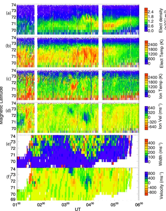
Observations of electron density, electron temperature, ion temperature and line-of-sight ion velocity from the ESR are presented in Fig. 2, panels (a) to (d), respectively. The spec-tral width and line-of-sight velocity data from the Finland CUTLASS radar are shown in panels (e) and (f) (the latitude range has been restricted to correspond to the ESR data in the other four panels). Negative (positive) velocities repre-sent flow directed away from (towards) the Finland radar for both the CUTLASS and ESR data. An approximate conver-sion for UT to MLT for the CUTLASS Finland and EISCAT

70 71 72 73 74 70 71 72 73 74 70 71 72 73 74 70 71 72 73 74 70 71 72 73 74 70 71 72 73 74 70 71 72 73 74 70 71 72 73 74 70 71 72 73 74 70 71 72 73 74 0100 ₀₂00 ₀₃00 ₀₄00 ₀₅00 ₀₆00 UT 69 70 71 72 73 74 0100 ₀₂00 ₀₃00 ₀₄00 ₀₅00 ₀₆00 UT 69 70 71 72 73 74 0.0 0.6 1.2 1.8 2.4 0 600 1200 1800 2400 0 600 1200 1800 2400 -640 -320 0 320 640 0 100 200 300 400 -800 -400 0 400 800 V el oc ity ( m s -1) W id th ( m s -1) Io n V el ( m s -1) Io n T em p (K ) E le ct T em p (K ) E le ct d en si ty (x 10 11 m -3) M ag ne tic L at itu de (a) (b) (c) (d) (e) (f)

Fig. 2. Data from 20 December 1998, 01:00 UT to 06:00 UT. Panels (a) to (d) are observations from the ESR radar, electron density, electron

temperature, ion temperature and ion line-of-sight velocity (negative values are towards the radar) respectively. Panel (e) shows CUTLASS Finland, beam 9, spectral width data and panel (f) shows the beam 9 line-of-sight velocity (negative values are away from the radar).

fields-of-view is achieved by adding ∼2.5 h to the UT (the di-rect conversion is given by: (MLT in hours) = (UT in hours) −4.73 + (magnetic longitude in degrees)/15). There were two regions of high and variable spectral width in the CUT-LASS Finland data within this latitude and time range. The first started at 01:30 UT and moved poleward out of the lati-tude range shown at 02:30 UT. The second started where the equatorward edge of the high spectral width moved back to below 74◦N at 03:00 UT and finished with the equatorward edge moving poleward beyond 74◦N at 04:45 UT. These re-gions of high width roughly coincide with rere-gions of elevated and structured electron temperature, more noticeably in the second interval.

An analysis of the data between 71◦N and 72◦N has been conducted to determine the relationship between spatially and temporally coincident measurements of electron and ion temperature from the EISCAT and ESR radars and the spec-tral width measurements from CUTLASS Finland. This band of latitude has been chosen as the altitude of the EISCAT and ESR measurements are close to 300 km. The CUTLASS Finland observations in this region were also expected to be from around this height in the F-region. An investigation of the elevation angle data confirms that the scatter originates in the F-region. Coincident data from the EISCAT radars and the CUTLASS Finland radar during the interval 01:00 to 06:00 UT are plotted in Fig. 3 as a scatter plot for data bins

Spectral Width, ms-1 El ec tr o n T em p er at u re , K Io n T em p er at u re , K 0 2 4 6 8 10 12 14 No. of occurrences (a) (b) (c)

Electron temperature Ion temperature

3000 2500 2000 1500 3000 2500 2000 1500 3000 2500 2000 1500 3000 2500 2000 1500 3000 2500 2000 1500 3000 2500 2000 1500 0 100 200 300 400 500 100 200 300 400 500

Fig. 3. Left column is electron temperature from the two

main-land EISCAT beams and the ESR beam, vs. spectral width from the CUTLASS Finland radar. The data is restricted to 71◦to 72◦ latitude AACGM to cover only a small range of altitudes in the F-region from all of the radar beams. Row (a) EISCAT beam 1, (b) EISCAT beam 2, and (c) ESR. The right column shows the same but for ion temperature.

of 100 K (in the electron (or ion) temperature) and 25 ms−1 (in the HF spectral width). The occurrence in each bin is then colour coded to indicate where most of the observations lie. The comparison of spectral width with electron temper-ature is in the left hand column and with ion tempertemper-ature in the right hand column. Figures 3a–c show the comparison for beams 1 and 2 of the VHF radar and the ESR beam, re-spectively. There is a relationship between electron tempera-ture and spectral width apparent in Fig. 3; when the electron temperature is low there were very few occurrences of high spectral width. There appears to be no obvious, similar trend for the ion temperature in this interval.

Figure 4 shows a time series comparison from the VHF beam 1, gate 1 (gate numbering starting at 0 closest to the radar) and CUTLASS Finland, beam 7, gate 29 which corre-spond to approximately 71.4◦N and 300 km altitude. The HF spectral width is shown in red (right-hand axis), the electron temperature from EISCAT is in black and the ion tempera-ture from EISCAT is shown as the dotted blue line (both on the left-hand axis scale). This comparison further demon-strates that values of high spectral width (>200 ms−1)

coin-1000 1500 2000 2500 3000 T e m p e ra tu re , K 0 200 400 600 S p e ct ra l W id th , (m s -1) 0100 ₀₂00 ₀₃00 ₀₄00 ₀₅00 UT 0600 E lectron T emp Ion T emp Width

Fig. 4. Line plots from collocated radar cells of EISCAT beam 1 and

beam 9 of CUTLASS Finland, within the 71◦N to 72◦N (AACGM) latitude range. Electron temperature is in black, ion temperature in blue (dotted) and spectral width is in red.

cided with high electron temperature in this interval. The region of wave activity seen in the CUTLASS Fin-land line-of-sight velocity from 02:00 UT to 04:10 UT was believed to be a field line resonance (FLR) by Woodfield et al. (2002). Combined with magnetometer measurements of the FLR from the IMAGE chain (Viljanen and Hakkinen, 1997) the OCFLB was given a lower limit of 72.9◦N for the time span 02:00 UT to 06:00 UT in Woodfield et al. (2002). This conclusion was based on the fact that FLRs are only ob-served on closed field lines. Thus we can reasonably assume that the scatter plots in Fig. 3 are all derived from closed field line phenomena.

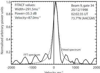
Figure 5 presents an example of CUTLASS Finland broad (291.5 ms−1) single peak spectrum for range gate 34 of beam 9 (approximately 73.7◦N) taken from the scan of beam 9 at 02:02:35 UT (this fast Fourier transform (FFT) of the ACF has been normalised). The fitted, normalised power spectrum for the FITACF parameters of velocity and width has been overlaid for comparison, where an exponentially decaying ACF has been assumed (Villain et al., 1987). The power fitted by FITACF, 35.3 dB, was high and well above noise levels (>3 dB). The majority of the spectra with high spectral width had only one peak (the number of peaks be-ing defined here as those peaks with power above half that of the maximum peak). In the high spectral width regions the tendency was for either a cluster of spectra with many peaks to occur over several minutes and range gates or for

-2000 -1000 0 1000 2000 Velocity, ms-1 0.2 0.4 0.6 0.8 1.0 N o rm al is ed a rb it ra ry p o w er u n it s FITACF values: Width=291.5ms-1 Power=35.3 dB Velocity=87.0ms-1 Beam 9, gate 34 20/12/1998 02:02:35 UT 73.7o_{N (AACGM)} Fitted spectrum FFT spectrum

Fig. 5. A typical normalised power spectrum (FFT of the ACF)

from the high spectral width region observed by CUTLASS Fin-land on 20 December 1998. This spectrum is from beam 9, gate 34 (∼73.7◦N AACGM) at 02:02:35 UT. A fitted spectrum for the FITACF parameters (assuming an exponential ACF) is overlaid as the dashed line.

spectra with two (sometimes three peaks) to be dotted in amongst the single spectra. There was a cluster of multiple-peak spectra at latitudes greater than 73◦_{N in the period} 02:00 UT to 02:30 UT. However, in the region 71◦N to 72◦N (roughly gates 29 to 31 for beam 9 of CUTLASS Finland) where the scatter analysis was conducted, there were virtu-ally no instances of multiple-peak spectra.

3.2 22 to 23 November 1999

During the interval 20:00 UT on 22 November 1999 to 06:00 UT on 23 November 1999 the WIND spacecraft was located at approximately (−13, −67, 15) RE in (x, y, z) GSM coordinates. Data from the WIND MFI and SWE in-struments are described below (data not shown) (Lepping et al., 1995; Ogilivie et al., 1995). The time delay from obser-vation at the spacecraft until incidence on the magnetopause is estimated at 3 ± 15 min. From 20:00 UT to 03:30 UT Bz(GSM) varied between 0 and +6 nT. From 03:30 UT Bz moved almost linearly from 0 nT to −8 nT at 06:00 UT when it turned sharply northwards again within a few minutes. The By component was positive and relatively large (+4 to +7 nT) from 20:00 UT until 02:00 UT, when it became ∼0 nT for 30 min before rising steadily to +7 nT at 03:30 UT. It remained at +7 nT until 04:30 UT when it decreased to −4 nT at 06:00 UT and then turned sharply in a few min-utes to +8 nT. The solar wind velocity was 450 ±20 ms−1 throughout the interval. The proton density was steady at ∼6 cm−3 from 20:00 UT to 03:00 UT after which 3 bursts of enhanced density occurred, each approximately 1 h in duration and 12 cm−3 in magnitude. In summary, the so-lar wind and interplanetary magnetic field (IMF) conditions were relatively stable with Bznorthwards from 20:00 UT un-til ∼03:30 UT when there was a steady change to Bz

south-wards passing 0 nT at 04:00 UT.

Data from the x-component of the IMAGE network (not shown) indicated quiet conditions until ∼00:45 UT when there was a deflection in the magnetic signature at the Bear Island station (BJN, 71.3◦N) of −100 nT from the mean field value. This was the station where the largest deflection was seen, smaller deflections were seen poleward and equator-ward, decreasing in magnitude the further in latitude away from BJN. The x-component at BJN returned to previous values at 02:30 UT when wave activity with an amplitude of ∼25 nT and frequency of ∼2 mHz ensued in the stations from BJN to Ny Alesund (NAL, 76.0◦N). Similar patterns were seen in the stations south of BJN, but of smaller am-plitude ∼10 nT. This wave activity continued around a con-stant and small, 0–25 nT, offset from the mean field, un-til 05:20 UT when a sharp, short-lived (∼5 min) bay in the x-component occurred. The bay was negative from Han-kasalmi (HAN, ∼58.5◦_{N) to Sørøya (SOR, ∼67.1}◦_{N) and} positive from BJN to NAL. Following this bay, all of the measured x-components steadily decreased. The magnitude of the change was largest at BJN where the deflection started at ∼0 nT at 05:20 UT to ∼100 nT at 06:00 UT and then in-creased in the same manner from the minimum at 06:00 UT. During this decrease, the stations from SOR to Ouluj¨arvi (OUJ, ∼60.8◦N) observed a wave signature (∼30 nT tude from 05:20 UT to 05:30 UT, then with a smaller ampli-tude to 06:00 UT) with a frequency of ∼4 mHz in all three components. The amplitude of this wave was much reduced at all the stations north of SOR, similar to the wave signature observed in the first case study. It seems likely that this was another FLR, although not as clear an example as the previ-ous case, making it harder to identify where the last closed field line was. Fortunately, as will be described shortly, there was another signature of the OCFLB available to us in the EISCAT data which we have used.

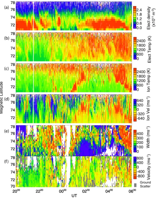
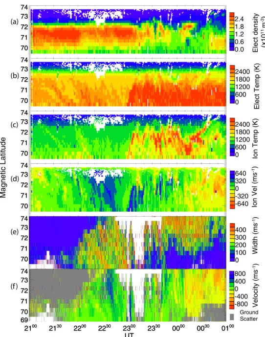
Figure 6 presents data from this interval from beam two of the EISCAT VHF radar and beam 9 of CUTLASS Fin-land for the latitude range 70◦N to 78◦. Panels (a) to (d) of Fig. 6 present the electron density, electron temperature, ion temperature and line-of-sight ion velocity from the EISCAT VHF beam 2, respectively (equivalent to altitudes of approxi-mately 280 to 510 km). From 20:00 UT to 23:00 UT the elec-tron density in the latitude range 70.5◦N to 74◦N was large (> 2.7 × 1011m−3). At 23:00 UT the electron density de-creased, although remaining structured, until 02:00 UT when it returned to levels prior to 23:00 UT. The electron temper-ature observations (Fig. 6b) exhibited complex structuring from 23:00 UT until the end of the interval at all latitudes. The electron temperature enhancements at 23:00 UT coin-cided with the first evidence of enhanced ion temperature which appeared to move equatorward (panel c). The sub-sequent electron temperature enhancements (after 02:00 UT) were particularly large. From panel (c) we have identi-fied three intervals when strong and consistent ion frictional heating was observed. Ion frictional heating occurs when the imposed electric field changes direction or magnitude. This changes the ion flow vector Vi, but has little immediate

72 74 76 78 72 74 76 78 72 74 76 78 72 74 76 78 72 74 76 78 72 74 76 78 72 74 76 78 72 74 76 78 72 74 76 78 72 74 76 78 2000 ₂₂00 ₀₀00 ₀₂00 ₀₄00 ₀₆00 UT 70 72 74 76 78 2000 ₂₂00 ₀₀00 ₀₂00 ₀₄00 ₀₆00 UT 70 72 74 76 78 M ag ne tic L at itu de 0.0 0.6 1.2 1.8 2.4 0 600 1200 1800 2400 0 600 1200 1800 2400 -640 -320 0 320 640 0 100 200 300 400 -800 -400 0 400 800 V el oc ity ( m s -1) W id th ( m s -1) Io n V el ( m s -1) Io n T em p (K ) E le ct T em p (K ) E le ct d en si ty (x 10 11 m -3) Ground Scatter (a) (b) (c) (d) (e) (f)

Fig. 6. Data from 22 to 23 November 1999. Panels (a) to (d) incoherent scatter data from EISCAT beam 2, 359◦, electron density, electron

temperature, ion temperature and ion line-of-sight velocity (negative values are away from the radar), respectively. Panel (e) spectral width from beam 9 of CUTLASS Finland, and panel (f) line-of-sight velocity (negative values are away from the radar) from the same.

effect on the velocity of the more numerous neutral atoms, Vn. The ions then collide with the neutrals causing an ion temperature enhancement that is proportional to the square of the vector difference, (Vi −Vn)2. Momentum transfer from ions to neutrals (ion drag) causes the neutral velocity Vnto become more aligned (in both magnitude and direction) with the new velocity and thus (Vi−Vn)2and the ion heat-ing is reduced (e.g. Rees and Walker, 1968; St-Maurice and Hanson, 1982; Davies et al., 1999). The first of the ion fric-tional heating signatures was the equatorward moving feature that moved from 76◦N at 23:00 UT to 70.5◦N at 23:30 UT. This was a weak signature that was collocated with a

veloc-ity shear presented in panel (d). The second ion frictional heating signature started at 70.5◦N at 00:45 UT and moved steadily poleward reaching 75◦N at 01:30 UT. The third ion frictional heating signature moved equatorward from 76.0◦N at 04:15 UT to 70.5◦N at 06:00 UT. These last two features were in the same region as shearing in the velocity as well as depletions in the F-region electron density. In general, the line-of-sight ion velocities were highly variable and struc-tured during this interval.

Previously Lockwood et al. (1988) have shown that such moving bands of ion frictional heating associated with ve-locity shear such as those identified above, follow the motion

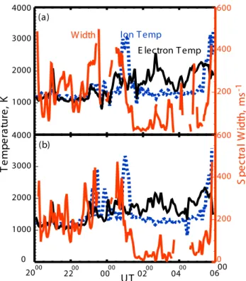
1000 2000 3000 4000 200 400 600 0 1000 2000 3000 4000 T e m p e ra tu re , K 0 200 400 600 S p e ct ra l W id th , m s -1 (a) (b) E lectron T emp Ion T emp Width 2000 2200 0000 _UT0200 0400 0600

Fig. 7. Line plots from overlapping radar cells between (a)

EIS-CAT beam 1, and (b) EISEIS-CAT beam 2, and appropriate CUTLASS Finland range cells, within the 71◦N to 72◦N latitude range. Elec-tron temperature is in black, ion temperature in blue (dotted) and spectral width is in red.

of the FRB. The width of the ion frictional heating region is controlled by the length of time for which the difference in velocity between the ions and neutrals is significant and hence (Vi−Vn)2is large. If the electric field conditions re-main stable then the width of the ion frictional heating band will reflect the length of time it takes the neutrals to align with the ions. When the polar cap is contracting (expand-ing) the FRB is the poleward (equatorward) edge of the re-gion of hot ions (Lockwood and Fuller-Rowell, 1987a, b). In this case study it seems reasonable to use these ion frictional heating signatures (particularly the last two) as ionospheric proxies for the FRB. The FRB can in turn be used as a rep-resentation of the OCFLB. The FRB will always be equa-torward of or equal to the latitude of the OCFLB with two possibilities to cause separation of the two. Regions of high conductivity such as may well occur in the auroral region equatorward of the OCFLB tend to cause a deviation in the plasma flow such that it avoids the high conductivity region and thus moving the FRB equatorward also. The second pos-sibility is viscous interaction with a convection cell on closed field lines, close to the OCFLB (e.g. Lockwood et al., 1988). Fox et al. (1994) demonstrated how such viscous cells could actually often be driven by nightside reconnection, as sug-gested by Lockwood and Cowley (1992). Therefore, when the polar cap is contracting the poleward edge of the region of hot ions shows is a reasonable proxy for the OCFLB, but when the polar cap is expanding the equatorward edge of the

hot ions can be on closed field lines and so can be considered as the minimum latitude limit for the OCFLB

Figure 6f presents the line-of-sight velocity from CUT-LASS Finland beam 9. The overall form of the CUTCUT-LASS velocity data was similar to that from the VHF system in Fig. 6d. The CUTLASS and VHF velocity data both show very complex flows from 20:00 UT to 00:15 UT. An inves-tigation of the global plasma velocity pattern during this time was performed using the spherical harmonic potential fitting of the “potential map” technique (Ruohoniemi and Baker, 1998), utilising all the northern hemisphere Super-DARN radars. The flow patterns from 20:00 UT to 23:00 UT were highly complex, although it appeared that the locations of the EISCAT and CUTLASS radar beams were essentially in the region of anti-sunward flow out of the polar cap and as such the location of the FRB could not be located unam-biguously during this time. The CUTLASS data indicated that the FRB was close to 70◦_{N shortly after 23:30 UT and} remained there until the majority of the ionospheric scat-ter disappeared at 00:15 UT. When the ionospheric scatscat-ter returned at 00:30 UT the FRB identified from spatial plots of the CUTLASS line-of-sight velocities from both radars moved poleward following the motion of the second ion fric-tional heating signature. The latitude range of particular in-terest is 71◦N to 72◦N as this is the latitude range in which direct comparison between electron temperature and spectral width is made. The OCFLB was located poleward of 72◦N from 20:00 UT to ∼23:15 UT (also reasonable since the pre-vailing IMF and solar wind conditions would indicate that the polar cap was reasonably small at this time), from 23:15 UT to ∼01:15 UT the OCFLB was equatorward of 72◦_{N, then} for the remainder of the interval (01:15 to 06:00 UT) the OCFLB was located poleward of 72◦_{N. This interpretation} agrees with that obtained from the ion frictional heating sig-natures, namely that in the latitude range 71◦N to 72◦N the field lines are closed from 20:00 UT to 23:15 UT, open from 23:15 UT to 01:15 UT and closed again from 01:15 UT to 06:00 UT.

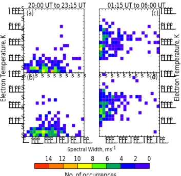
To consider the HF spectral width data in Fig. 6e we have split the dataset into two distinct subintervals, 20:00 to 23:15 UT and 01:15 to 06:00 UT. The first of these subinter-vals contained a large region of high spectral width with an ill-defined boundary. In the second, a very definite boundary between high and low spectral width existed and moved in latitude with time. Thus we avoid the interval of open field lines from 23:15 UT to 01:15 UT. The HF spectral width in the first subinterval (20:00 to 23:15 UT) did not appear to be related to any elevated electron temperatures. In the second subinterval a well defined gradient in the spectral width was evident, with high values poleward of low values. The equa-torward boundary of the region of high spectral width fol-lowed the motion of the velocity shear and previously iden-tified ion frictional heating features where they were present. In between the last two ion frictional heating features (01:15 to 06:00 UT) the high values of spectral width appear to be related more to the electron temperature enhancements, as in the first case study.

20:00 UT to 23:15 UT 01:15 UT to 06:00 UT (a) (b) (c) (d) Spectral Width, ms-1 El ec tr o n T em p er at u re , K 0 2 4 6 8 10 12 14 No. of occurrences 3000 2500 2000 1500 3000 2500 2000 1500 3000 2500 2000 1500 3000 2500 2000 1500 0 100 200 300 400 500 100 200 300 400 500 El ec tr o n T em p er at u re , K

Fig. 8. Electron temperature from the EISCAT mainland beams

vs. spectral width from the CUTLASS Finland radar, the data is restricted to 71◦ to 72◦ latitude AACGM. Left column, data from 20:00 UT to 00:15 UT, right column, data from 00:15 UT to 06:00 UT. Top row, EISCAT beam 1, bottom row, EISCAT beam 2.

The very different nature of the two subintervals of spec-tral width behaviour becomes apparent when comparing the time series for collocated EISCAT and CUTLASS Finland data. This has been done for both the VHF beams and is presented in Fig. 7a beam 1 (gate 1, ∼71.4◦_{N corresponding} to beam 7, gate 29 of CUTLASS Finland) and (b) beam 2 (gate 1, ∼71.3◦N corresponding to beam 8, gate 28 of CUT-LASS Finland). As in the first study, a height of 300 km is assumed since the elevation angle is indicative of F-region scatter. As before, the spectral width is in red, electron tem-perature is in black and ion temtem-perature is in blue (dotted). At 00:15 UT in both VHF beams there is a large spike in the ion temperature corresponding to the poleward motion of the re-gion of ion frictional heating. As this passes through the lat-itude from which these cells are taken, the spectral width be-haviour changes distinctly from being high to being generally low. Then, a few minutes after 05:30 UT when the ion fric-tional heating returned equatorward, the spectral width ap-peared to be returning to its former wider behaviour just be-fore 06:00 UT. Within the interval of 01:15 UT to 06:00 UT, the OCFLB is poleward of the cells from which the data in Fig. 7 is taken, thus the observations were again made on closed field lines. The scatter plots for electron temperature and HF spectral width generated in the same way as for the first case study are presented in Fig. 8. The ion temperature comparison in the region 71◦N to 72◦N is similar to that in Fig. 3 (i.e. with no clear effect on spectral width) and is therefore not shown here. The ion frictional heating signa-tures pass through this region only briefly and thus the ob-served correspondence between large spectral width and the

0.2 0.4 0.6 0.8 1.0 N o rm al is ed a rb it ra ry p o w er u n it s FITACF values: Width=394.5ms-1 Power=36.7 dB Velocity=-65.9 ms-1 Beam 9, gate 31 23/11/1999 00:52:42 UT 72.5o_{N (AACGM)} Fitted spectrum FFT spectrum -2000 -1000 0 1000 2000 Velocity, ms-1 0.2 0.4 0.6 0.8 1.0 FFT spectrum Fitted spectrum FITACF values: Width=336.7ms-1 Power=33.3 dB Velocity=-389.9 ms-1 Beam 9, gate 30 23/11/1999 00:52:42 UT 72.0o_{N (AACGM)} (a) (b)

Fig. 9. Two typical normalised power spectra (FFT of ACF)

from the high spectral width region observed by CUTLASS Fin-land on 23 November 1999. These spectra are from beam 9, (a) gate 31 (∼72.5◦N AACGM), (b) gate 30 (∼72.0◦N AACGM) at 00:52:42 UT. Fitted spectra for the FITACF parameters (assuming an exponential ACF) are overlaid as dashed lines.

ion frictional heating does not show up in a scatter plot anal-ysis. Figure 8 panels (a) and (b) show the relationship during the interval 20:00 to 23:15 UT and panels (c) and (d) show the data from 01:15 UT to 06:00 UT. The upper panels (a) and (c) are for EISCAT beam 1, the lower panels (b) and (d) are for beam 2. There are two different relationships demon-strated by these figures. The data from 01:15 UT to 06:00 UT, when the observations were from a closed field line region, show a similar pattern to that found in the first case study, while the other data (20:00 to 23:15 UT) show virtually no relationship with HF spectral widths: spectral widths (low and high) are seen but at low electron temperatures.

Figure 9 shows two typical types of spectra from the HF scatter region with high spectral width during the second ion frictional heating event. Panel (a) shows a very wide but sin-gle peak spectrum from gate 31 of beam 9 (∼72.5◦N) and panel (b) show a similarly wide spectrum from gate 30 of beam 9 (∼72.0◦N) but with two main peaks. Both spec-tra are from the same scan of beam 9 at 00:52:42 UT. As in Fig. 5, the spectra are normalised and a fitted spectrum produced from the FITACF values is overlaid for

2100 ₂₁30 ₂₂00 ₂₂30 ₂₃00 ₂₃30 ₀₀00 ₀₀30 ₀₁00 UT 2100 ₂₁30 ₂₂00 ₂₂30 ₂₃00 ₂₃30 ₀₀00 ₀₀30 ₀₁00 UT Ground Scatter 70 71 72 73 74 70 71 72 73 74 70 71 72 73 74 70 71 72 73 74 70 71 72 73 74 70 71 72 73 74 70 71 72 73 74 70 71 72 73 74 70 71 72 73 74 70 71 72 73 74 69 70 71 72 73 74 69 70 71 72 73 74 0.0 0.6 1.2 1.8 2.4 0 600 1200 1800 2400 0 600 1200 1800 2400 -640 -320 0 320 640 0 100 200 300 400 -800 -400 0 400 800 V el oc ity ( m s -1) W id th ( m s -1) Io n V el ( m s -1) Io n T em p (K ) E le ct T em p (K ) E le ct d en si ty (x 10 11 m -3) M ag ne tic L at itu de (a) (b) (c) (d) (e) (f)

Fig. 10. Data from 21 to 22 August 1998. Panels (a) to (d) are observations from the ESR radar, electron density, electron temperature,

ion temperature and ion line-of-sight velocity (negative values are towards the radar) respectively. Panel (e) shows CUTLASS Finland, beam 9, spectral width data and panel (f) shows the beam 9 line-of-sight velocity (negative values are away from the radar) both at high time resolution.

son. This figure demonstrates the variability in the number of peaks of the spectra seen in high spectral width regions and how large widths can come from both single and mul-tiple peak spectra. Panel (b) also demonstrates that when the spectrum has more than one peak the FITACF veloc-ity does not show the whole story. This is generally re-flected by an increase in the parameter which indicates the estimated error in the FITACF fitting (Andr´e et al., 2000a). In particular the third ion frictional heating signature (from 04:15 UT to 06:00 UT) has very large spectral widths, often over 1000 ms−1. The spectra from this last heating signa-ture have typically more than one peak (again identifying the

number of peaks in the spectrum as those with more than or equal to half the power or the main peak). This phe-nomenon has been well studied on the dayside in the cusp (e.g. Andr´e et al., 1999; 2000a). In the regions where there is no ion frictional heating essentially all the HF spectra are single peaks with only a few being multiple-peak. All the other high spectral widths from the entire interval are as in the previous case study, mainly single-peak spectra with a few double or triple peak spectra distributed widely. The very high spectral widths at the end of the interval from ∼04:30 UT could be related to the cusp since the strongly positive By component in the IMF would shift the cusp to

earlier MLT. There are several indicators that this could be cusp data even at this early MLT (04:30–06:00 UT corre-sponds to about 06:45–08:15 MLT): the presence of large and variable spectral widths in the CUTLASS data (e.g. Baker et al., 1995), the poleward moving forms in the velocity data (this is clearer in the EISCAT ion velocity data) (e.g. Thorolfsson et al., 2000; Lockwood et al., 2000), the increase in electron density following the depletion due to the passage of the ion frictional heating region (likely due to cusp precip-itation, Yeoman et al., 1997; Newell and Meng, 1992). Per-haps most indicative is the oppositely directed motion of the FRB and the ions from ∼04:30 UT. This behaviour is con-sistent with a non-adiaroic OCFLB implying that there is re-connection occurring in this local time sector which opens field lines and moves them into the polar cap. It is hard to separate the spectra found in the presence of ion frictional heating and those located in the cusp in this final part of the data, indeed some of the ion frictional heating may be due to large flows observed in the cusp. However, the more pole-ward in the region of hot ions one looks, the more clustered the multiple-peak spectra are and the more peaks they have. It seems likely therefore, that the truly multiple-peak spec-tra are related to the cusp, and in the region of ion frictional heating the spectra are single, double and occasionally triple-peak.

3.3 21 to 22 August 1998

The final case study presented here is taken from 21:00 UT on 21 August 1998 to 01:00 UT on 22 August 1998. The ionospheric flows in this interval have been studied previ-ously as an example of isolated substorm plasma flow be-haviour (Yeoman et al., 2000). The CUTLASS Finland radar was running a high time resolution mode on beam 9 which is ideal for comparison with the low elevation mode of the ESR that was running during the SP-UK-CSUB EISCAT and ESR campaign at that time. The mainland EISCAT VHF system was running in split beam, CP4 type mode during the night time runs undertaken.

Data from the ESR are presented in Fig. 10 along with the high time resolution observations from beam 9 of CUT-LASS Finland. Panels (a) to (d) show electron density, elec-tron temperature, ion temperature and line-of-sight ion veloc-ity from the ESR data, respectively. Panels (e) and (f) show the spectral width and line-of-sight velocity from CUTLASS Finland beam 9. The onset of the substorm growth phase be-gins at ∼21:15 UT, with expansion onset from 22:50 UT and full recovery by ∼23:40 UT (Yeoman et al., 2000). There are two equatorward moving auroral forms observed between 21:20 and 22:20 UT in the electron and ion temperature data (panels (b) and (c) of Fig. 10). These features are typical of the growth phase of an isolated substorm (Persson et al., 1994). Then, after the expansion phase onset at 22:50 UT identified by Pi2 pulsations in the IMAGE ground magne-tometer network (Yeoman et al., 2000), there is a poleward expanding auroral form seen in the electron and ion temper-ature, the substorm associated auroral bulge. Given the large

(a)

(b)

(c)

El

ec

tr

o

n

T

em

p

er

at

u

re

, K

Electron temperature

N

o

. o

f o

cc

u

rre

n

ce

s

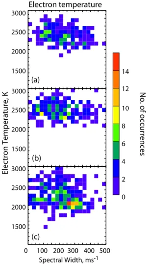
Fig. 11. Electron temperature from the two mainland EISCAT

beams and the ESR beam, vs. spectral width from the CUTLASS Finland radar. The data is restricted to 71◦to 72◦latitude AACGM to cover only a small range of altitudes in the F-region from all of the radar beams. Row (a) EISCAT beam 1, (b) EISCAT beam 2, and (c) ESR. 1.

line-of-sight ion velocities and F-region density depletion the elevated ion temperature is due to ion frictional heating. The ion frictional heating could indicate (as in the second case study) the motion of the FRB as the substorm expansion phase destroys open flux in the polar cap.

Once the CUTLASS Finland ionospheric scatter becomes predominant over the ground scatter at ∼21:40 UT the equa-torward edge of the region of scatter moves equaequa-torward in accordance with previous substorm growth phase studies (Lewis et al., 1997), although this is out of the latitude range of Fig. 10e and f. The line-of-sight velocities (where there is ionospheric scatter) are comparable to those seen by the ESR and VHF radar as shown by Davies et al. (2000), the ESR data is presented in Fig. 10d. Yeoman et al. (2000) as-cribed the first dropout of ionospheric data (at 23:00 UT) to a reduced number of irregularities due to suppressed elec-tric fields. The second (at 23:10 UT) they assume to be due to the changing HF propagation conditions as the substorm

progresses (Gauld et al., 2002). Then, as the substorm sub-sides, the ionospheric scatter returns and moves poleward.

The beam-swinging analysis performed by Yeoman et al. (2000) on the data from the two VHF beams indicates the location of the FRB for the majority of the interval from 22:30 UT to 23:30 UT. The FRB moves equatorward of 72◦N at approximately 22:45 UT and then returns pole-ward of 72◦N at about 23:05 UT, for the rest of the interval it would seem to be above 72◦N given the absence of mag-netic activity before the substorm onset and the expanded au-roral bulge later on. Little backscatter is observed between 71◦N and 72◦N during these 20 min, thus for the majority of the interval which is analysed and presented as a scatter plot of electron temperature and HF spectral widths as for the other two cases (Fig. 11), the data are from regions of the ionosphere threaded by closed field lines: Fig. 11a is for the EISCAT beam 1 data, Fig. 11b for the EISCAT beam 2 and Fig. 11c for the ESR. F-region scatter is assumed from the range of the data although the elevation angle data in this interval is unclear. The form of the relationship between electron temperature and spectral width does not resemble that of case study at all. Firstly the overall electron tempera-ture level is ∼1000 K higher than previously. This could be attributed to the increase in solar radiation due to the time of year although the electron density is not increased. Sec-ondly, there is no distinct absence of low spectral widths at high electron temperatures, as in the pre-midnight UT half of the second case study. If there is any dependence, it is that spectral widths decrease slightly with increased electron temperature.

The spectra observed in this final case study show many multiple-peak examples, particularly in the region of high spectral width observed from ∼23:45 UT in the main band of scatter from ∼70◦N to ∼75◦. It is interesting in this case that there are multiple-peak spectra in the presence of high spectral widths and elevated electron temperatures, but we do not see the relationship between high widths and high tem-peratures as in the first study. It is possible that the smaller integration time for the CUTLASS Finland data in this case is showing up more of the multiple-peak spectra that may not be observable in the larger integration times of the other cases.

4 Discussion

The three case studies presented in Sect. 3 cover a varied set of geophysical conditions all of which have high spec-tral width data from the CUTLASS Finland coherent HF radar. There is evidence that the turbulence creating these large widths is generated by more than one physical mech-anism, although it is possible to have a dominant mecha-nism. The evidence presented in the three case studies can be summarised in three key points, (i) high widths (>200 ms−1) originate from both single and multiple-peak spectra, (ii) the relationship between electron temperature and high spectral width is not consistent in the different intervals, and (iii)

high spectral width can occur on both open and closed field lines. That more than one generating mechanism probably exists is unsurprising in such a dynamically complex region as the ionosphere. The question following from this is can we associate particular mechanisms with specific geophysi-cal conditions and/or locations and perhaps specific forms of the power spectra. This has been done on the dayside with multiple-peak spectra associated with the cusp (Baker et al., 1995; Andr´e et al., 1999, 2000a) and for double-peak spec-tra associated with the LLBL (Schiffler et al., 1997; Huber and Sofko, 2000). The aim here is to apply similar proce-dures on the nightside. The physical mechanisms proposed for the dayside, namely temporal electric field variations in the Pc1/Pc2 frequency band (Andr´e et al., 1999, 2000a) and small scale vortices in the plasma (Schiffler et al., 1997; Hu-ber et al., 2000; Andr´e et al., 2000b) are equally applicable to the nightside.

The analysis of the 20 December 1998 case study indi-cates a relationship between electron temperature and spec-tral width, namely that high specspec-tral width is associated with elevated electron temperatures, but not vice versa. This anal-ysis took place at ∼300 km, 71◦N to 72◦N and on closed field lines in the post-midnight sector. The spectra that are observed in the region of high spectral width are primarily single-peak spectra with a cluster of multiple-peak spectra between 02:00 to 02:30 UT and ∼73◦N to ∼83◦N. There are more observations of multiple-peak spectra in the high spec-tral width region than in the low specspec-tral width region. In the region of detailed investigation between 71◦N and 72◦N there are virtually no multiple-peak spectra. Elevated elec-tron temperature in incoherent scatter radar data is a good indicator that there is particle precipitation present (Kofman and Wickwar, 1984) and this is often also related to field aligned currents. Since high spectral widths are associated with high electron temperatures in this interval in the region 71◦N to 72◦N, it is reasonable to say that the large spec-tral widths could be related to precipitation. It should be noted that this is not a straightforward conclusion, because there are many low spectral widths at high electron temper-atures, but there are no high spectral widths at low electron temperatures. Thus, at this time, elevated electron tempera-ture appears to be necessary, but not sufficient, to give high spectral widths. This perhaps shows us that several processes are in progress that have different effects on the ionospheric plasma. The lifetime and drift of the backscatter targets could have an effect on the data that were observed, however the lifetimes of the irregularities are short, of the order of sec-onds and will not have a large effect. It would appear, from the one-sided nature of the electron temperature to spectral width relationship, that not all high temperature electrons are related to large widths but high temperatures are required if there are to be large widths. This could lead to the conclu-sion that different processes are involved, one which shows up as high electron temperature and is related to large spec-tral widths and one which just has a high electron tempera-ture signatempera-ture. At this time we can only speculate as to what this difference maybe. If, for example, the high

tempera-ture is indicative of precipitation, then there could be vor-tices caused by the mechanism suggested by Schiffler and Sofko (2000). These would be discrete objects and may not cause large widths in every range cell analysed but would all be within the region of high electron temperature. There is also optical auroral activity in this region at this time veri-fying the presence of particle precipitation (Woodfield et al., 2002). Whether there is likely to be filamentary particle pre-cipitation, suitable for the generation of vortices of a scale size less than that of the radar cell, remains unclear, but the fact that precipitation is present is supporting evidence that high spectral widths may be generated in this fashion. The fact that there are almost no multiple-peak spectra in the re-gion 71◦N to 72◦N however, does not support the vortex idea and also the region of optical activity extends equator-ward of the high spectral width values. The comparison with ion temperatures is unrevealing except to say that there is no obvious correlation between the spectral width and the ion temperatures in this interval. As the second case shows, this is not always the case.

The second case study, 22 to 23 November 1999 is split into two parts, the first (20:00 UT to 23:15 UT) has a poorly defined boundary between high and low spectral width. The line of sight velocities in this interval are also highly vari-able indicating a highly turbulent plasma environment. The vast majority of the coherent power spectra in this part of the interval have only one peak indicating that neither the tem-poral electric field, nor the vortex mechanism for generating high spectral width is likely to be present. It seems that the high spectral width is due simply to the variation of the line-of-sight velocity about a central value during the integration time in a regime where the velocity is very variable. The analysis of electron temperature and spectral width for this part of the interval indicates no clear relationship between the two parameters. This is not to say that there is no precip-itation going on as the structure in the electron density and electron temperature indicate that there most likely is precip-itation. The first subinterval of this case study is probably on closed field lines given the geophysical conditions and the possible FRB motion equatorward at ∼23:00 UT (shown in the ion temperature) during this time. This conflicts with the first case study electron temperature comparison results since that was also on closed field lines. The main difference be-tween these two intervals is the data location in MLT, in this case the data are from the pre-midnight sector.

The second part of the interval (from 01:15 UT to 06:00 UT) has a clear example of ion frictional heating at a velocity shear indicating the location of the FRB. This in turn gives an approximate location for the OCFLB. The be-haviour of the spectral width parameter changes dramatically as the FRB passes poleward of the region being analysed. Once the analysis is on closed field lines again (01:15 UT to 06:00 UT) the relationship of electron temperature to tral width is similar to the first case study. The power spec-tra at the latitudes being analysed for this relationship again have mainly single peaks. Therefore, as in the first interval, there is no evidence for the presence of vortices in the region

where we find the large spectral widths are related to high electron temperatures. However, the power spectra in the re-gion of the second ion frictional heating event and FRB have more than one peak (typically two peaks) and such a velocity shear could cause vortices by the Kelvin-Helmholtz instabil-ity. In the last hour and a half of the data it is difficult to tell which of the spectra are related to ion frictional heating and which are due to the cusp. The spectral width parameter from the FITACF software in this last section of the data is very large as FITACF reaches the limits of its ability to fit to these difficult spectra. It is likely that part of this is early cusp activity due to the large, positive Byat this time. Other indi-cations that these data are from the cusp are the presence of poleward moving forms (e.g. Thorolfsson et al., 2000; Lock-wood et al., 2000), the increase in electron density probably due to soft precipitation such as is observed in the cusp re-gion (Yeoman et al., 1997; Newell and Meng, 1992), and the rotational (as opposed to shear) nature of the FRB at this time, indicating a non-adiaroic OCFLB at this time.

The third case study is an example of spectral width be-haviour during an isolated substorm following a prolonged period of northwards IMF. The previous two case studies considered alone would lead one towards the conclusion that the electron temperature to spectral width relationship found in the first case study happens on closed field lines. The third case study does not give the same result, on this occa-sion there is no obvious relationship between the two param-eters, despite the analysis being performed on closed field lines for the vast majority of the data. This may be related to the overall higher electron temperature, in general nearly 1000 K larger than the other two studies. This could be due to the time of year in which this case study occurs. The so-lar illumination, and hence atmospheric ionisation, is high in August whereas in the other two studies, conducted in late November and December, the illumination is low. Although one might expect the observed electron density to also be increased in summer, this need not be the case since other processes may deplete the electron density. In particular, in this case there is ion frictional heating also present and this is known to reduce the electron density. The spectra are also somewhat different in this case, showing more multiple-peak examples.

The first case study and the second part of the second study are the times during which there is a coincidence be-tween elevated electron temperature and the high HF spec-tral width. These intervals are both approximately located between 03:00 MLT and 08:00 MLT whereas the other inter-vals are in the range 22:00 MLT to 03:00 MLT. The discrimi-nating factor seems to be whether the data are from before or after ∼03:00 MLT on the nightside. The physical origin of this difference is not clear.

5 Summary

Three intervals of data with combined measurements from the CUTLASS Finland coherent HF radar and the EISCAT

and ESR radars have been investigated. A comparative ana-lysis of electron temperature data from the incoherent scat-ter radars and spectral width data from the Finland coherent radar performed at an altitude of ∼300 km, 71◦N to 72◦N finds a relationship between the two parameters in two of the case studies. The following key points have been identified:

(1) The relationship between electron temperature from the incoherent radar data and spectral width from the coher-ent radar data is not unique, nor is it universal. It appears to occur on closed field lines in the range 03:00 MLT to 08:00 MLT (08:00 MLT is the limit of the observations presented here).

(2) The power spectra from the coherent radar in the regions of high spectral width have both single and multiple-peaks. In general the single, wide peaks dominate. (3) The regions of high spectral width occur on both open

and closed field lines.

(4) The ion frictional heating in case study two is associated with large spectral widths in coherent radar data with more multiple-peaked spectra.

(5) Several causes of high spectral width on the nightside seem to exist, therefore its use as an ionospheric proxy must be approached with caution. The geophysical con-ditions and magnetic local time locations where it could perhaps be used as a proxy must be investigated further. Acknowledgements. The authors wish to thank those involved in

the deployment and operation of the CUTLASS HF radars run by the University of Leicester with joint funding from the UK Parti-cle Physics and Astronomy Research Council (PPARC) grant num-ber PPA/R/R/1997/00256, the Swedish Institute for Space Physics, Uppsala and the Finnish Meteorological Institute, Helsinki, the in-stitutes who maintain the IMAGE magnetometer array, R. Lep-ping at NASA/GSFC and CDAWeb for WIND data. EEW is in-debted to PPARC for a research studentship. JAD is supported by PPARC grant number PPA/G/O/1999/00181. EISCAT is an inter-national facility funded collaboratively by the research councils of Finland (SA), France (CNRS), the Federal Republic of Germany (MPG), Japan (NIPR), Norway (NAVF), Sweden (NFR) and the UK. (PPARC).

The Editor in chief thanks N. Sato and J. Moen for their help in evaluating this paper.

References

Andr´e, R., Pinnock, M., and Rodger, A. S.: On the SuperDARN autocorrelation function observed in the ionospheric cusp, Geo-phys. Res. Lett., 26, 22, 3353–3356, 1999.

Andr´e, R., Pinnock, M., and Rodger, A. S.: Identification of the low-altitude cusp by Super Dual Auroral Radar Network radars: A physical explanation for the empirically derived signature, J. Geophys. Res., 105, A12, 27 081–27 093, 2000a.

Andr´e, R., Pinnock, M., Villain, J.-P., and Hanuise, C.: On the factors conditioning the Doppler spectral width determined from SuperDARN HF radars, Int. J. Geomag. Aeronomy., 2, 1, 77–86, 2000b.

Baker, K. B. and Wing, S.: A new magnetic coordinate system for conjugate studies at high latitudes, J. Geophys. Res., 94, 9139– 9143, 1989.

Baker, K. B., Greenwald, R. A., Ruohoniemi, J. M., Dudeney, J. R., Pinnock, M., Newell, P. T., Greenspan, M. E., and Meng, C.-I.: Simultaneous HF-radar and DMSP observations of the cusp, Geophys. Res. Lett., 17, 11, 1869–1872, 1990.

Baker, K. B., Dudeney, J. R., Greenwald, R. A., Pinnock, M., Newell, P. T., Rodger, A. S., Mattin, N., and Meng, C.-I.: HF radar signatures of the cusp and low-latitude boundary layer, J. Geophys. Res., 100, A5, 7671–7695, 1995.

Davidson, G. T.: Expected Spatial Distribution of Low-Energy pro-tons Precipitated in the Auroral Zones, J. Geophys. Res., 70, 1061, 1965.

Davies, J. A., Lester, M., and McCrea, I. W.: Solar and seasonal dependence of ion friction heating, Ann. Geophys., 17, 682–691, 1999.

Davies, J. A., Yeoman, T. K., Lester, M., and Milan, S. E.: A com-parison of F-region ion velocity observations from the EISCAT Svalbard and VHF radars with irregularity drift velocity mea-surements from the CUTLASS Finland HF radar, Ann. Geo-phys., 18, 5, 589–594, 2000.

Dudeney, J. R., Rodger, A. S., Freeman, M. P., Pickett, J., and Scud-der, J., Sofko, G., Lester, M.: The nightside ionospheric response to IMF By changes, Geophys. Res. Lett., 25, 14, 2601–2604,

1998.

Greenwald, R. A., Baker, K. B., Dudeney, J. R., Pinnock, M., Jones, T. B., Thomas, E. C., Villain, J.-P., Cerisier, J.-C.,Senior, C.,Hanuise, C., Hunsucker, R. D., Sofko, G., Koehler, J., Nielsen, E., Pallinen, R., Walker, A. D. M., Sato, N., and Yamag-ishi, H.: DARN/SuperDARN: A global view of the dynamics of the high-latitude convection, Space Sci. Rev., 71, 761–796, 1995. Fox, N. J., Lockwood, M., Cowley, S. W. H., Freeman, M. P., Friis-Christensen, E., Milling, D. K., Pinnock, M., and Reeves, G. D.: EISCAT observations of unusual flows in the morning sector associated with weak substorm activity, Ann. Geophysicae, 12, 541–553, 1994.

Gauld, J. K., Yeoman, T. K., Davies, J. A., Milan, S. E., and Honary, F.: SuperDARN radar HF propagation and absorption response to the substorm expansion phase, Ann. Geophysicae, in press, 2002.

Gurnett, D. A., Huff, R. L., Menietti, J. D., Burch, J. L., Winning-ham, J. D., and Shawan, S. D.: Correlated Low-Frequency Elec-tric and Magnetic Noise Along the Auroral Field Lines, J. Geo-phys. Res., 89, 8971–8985, 1984.

Gurnett, D. A.: Auroral Plasma Waves, in: Auroral Physics, (Eds) Meng, C.-I., Rycroft, M. J., and Franck, L. A., chap. IV-6, Cam-bridge Univ. Press, New York, 241–254, 1991.

Huber, M. and Sofko, G. J.: Small-scale vortices in the high-latitude F region, J. Geophys. Res., 105, 20 885–20 897, 2000.

Kofman, W. and Wickwar, V. B.: Very high teperatures in the day-time F region at Sondestrom, Geophys. Res. Lett., 11, 919–922, 1984.

Lepping, R. P., Acuna, M. H., Burlaga, L. F., Farrell, W. M., Slavin, J. A., Schatter, K. H., Mariani, F., Ness, N. F., Neubauer, F. M., Whang, Y. C., Byrnes, J. B., Kennon, R. S., Panetta, P. V., Scheifele, J., and Worler, E. M.: The WIND magnetic field in-vestigation, Space Sci. Rev., 71, 207–229, 1995.

Lester, M., Milan, S. E., Besser, V., and Smith, R.: A Case Study of HF Radar Spectra and 630.0 nm Auroral Emission in the Pre Midnight Sector, Ann. Geophysicae, 19, 327–339, 2001.

Lewis, R. V., Freeman, M. P., Rodger, A. S., Reeves, G. D., and Milling, D. K.: The electric field response to the growth phase and expansion phase onset of a small isolated substorm, Ann. Geophysicae, 15, 289–299, 1997.

Lockwood, M. and Cowley, S. W. H.: Ionospheric Convection and the substorm cycle, in: “Substorms 1, Proceedings of the First In-ternational Conference on Substorms, ICS-1”, (Ed) Mattock, C., ESA-SP-335, European Space Agency Publications, Nordvijk, The Netherlands, 99–109, 1992.

Lockwood, M., Cowley, S. W. H., Todd, H., Willis, D. M., and Clauer, C. R.: Ion flows and heating at a contracting polar-cap boundary, Planet. Space. Sci., 36, 11, 1229–1253, 1988. Lockwood, M. and Fuller-Rowell, T. J.: The modelled occurrence

of non-thermal plasma in the ionospheric F-region and possible consequences for ion outflows into the magnetosphere, Geophys. Res. Lett., 14, 371, 1987a.

Lockwood, M. and Fuller-Rowell, T. J.: Correction to “The mod-elled occurrence of non-thermal plasma in the ionospheric F-region and possible consequences for ion outflows into the mag-netosphere”, Geophys. Res. Lett., 14, 581, 1987b.

Lockwood, M., McCrea, I. W., Milan, S. E., Moen, J., Cerisier, J. C., and Thorolfsson, A.: Plasma structure within poleward-moving cusp/cleft auroral transients: EISCAT Svalbard radar ob-servations and an explanation in terms of large local time extent of events, Ann. Geophysicae, 18, 1027–1042, 2000.

Matsuoka, A., Tsuruda, K., Hayakawa, H., Mukai, T., Nishida, A., Okada, T., Kaya, N., and Fukunishi, H.: Electric field fluctua-tions and charged particle precipitation in the cusp, J. Geophys. Res., 98, 11 225–11 234, 1993.

Maynard, N. C., Aggson, T. L., Basinka, E. M., Burke, W. J., Craven, P., Peterson, W. K., Suguira, M., and Weimer, D. R.: Magnetospheric boundary dynamics: DE-1 and DE-2 observa-tions near the magnetopause and cusp, J. Geophys. Res., 96, 3505–3522, 1991.

Milan, S. E. and Lester, M.: Interhemispheric differences in the HF radar signature of the cusp region A review through the study of a case example, Adv. in Polar Upper Atmos. Res., 15, 159–177, 2001.

Milan, S. E., Lester, M., Cowley, S. W. H., Moen, J., Sandholt, P. E., and Owen, C. J.: Meridian-scanning photometer, coherent HF radar, and magnetometer observations of the cusp: a case study, Ann. Geophysicae, 17, 159–172, 1999.

Moen, J., Carlson, H. C., Milan, S. E., Shumilov, N., Lybekk, B., Sandholt., P. E., and Lester, M.: On the collocation between dayside auroral activity and coherent HF radar backscatter, Ann. Geophysicae, 18, 1531–1549, 2001.

Newell, P. T. and Meng, C.-I.: Mapping the dayside ionopshere to the magnetosphere according to particle precipitation character-istics, Geophys. Res. Lett., 19, 609–612, 1992.

Ogilivie, K. W.,Chornay, D. J., Fritzenreiter, R. J., Hunsaker, F., Keller, J., Lobell, J., Miller, G., Scudder, J. D., Sittler Jr., E. C., Torbert, R. B., Bodet, D., Needell, G., Lazarus, A. J., Steinberg, J. T., Tappan, J. H., Mavretic, A., and Gergin, E.: SWE, A com-prehensive plasma instrument for the WIND spacecraft, Space Sci. Rev., 71, 55–77, 1995.

Persson, M. A. L., Aikio, A. T., and Opgenorth, H. J.: Satellite-ground coordination: late growth and Early expansion phase of a substorm, in: Proc. ICS-2, (Eds) Kan, J. R., Craven, J. D., and

Akasofu, S.-I., Fairbanks, USA, 1994.

Pinnock, M., Rodger, A. S., Dudeney, J. R., Rich, F., and Baker, K. B.: High spatial and temporal resolution observations of the ionospheric cusp, Ann. Geophysicae, 13, 919–925, 1995. Pinnock, M. and Rodger, A. S.: On determining the noon polar

cap boundary from SuperDARN HF radar backscatter character-istics, Ann. Geophysicae, 18, 1523–1530, 2001.

Rees, M. H. and Walker, J. C. G.: Ion and electron heating by auro-ral electric fields, Annales de Geophysique, 24, 193–199, 1968. Rishbeth, H. and Williams, P. J. S.: The EISCAT Ionospheric Radar:

the System and its Early Results, Q. J. R. Astr. Soc., 26, 478–512, 1985.

Rodger, A. S: Ground-based imaging of Magnetospheric bound-aries, Adv. Space Res., 25, No 7/8, 1461–1470, 2000.

Rodger, A. S., Mende, S. B., Rosenberg, T. J., and Baker, K. B.: Si-multaneous optical and HF radar observations of the ionsopheric cusp, Geophys. Res. Lett., 22, 2045–2048, 1995.

Ruohoniemi, J. M. and Baker, K. B.: Large-scale imaging of high-latitude convection with Super Dual Auroral Radar Network HF radar observations, J. Geophys. Res., 103, 20 797, 1998. Schiffler, A., Sofko, G., Newell, P. T., and Greenwald, R.:

Map-ping the outer LLBL with SuperDARN double-peaked spectra, Geophy. Res. Lett., 24, 3149–3152, 1997.

St-Maurice, J.-P. and Hanson, W. B.: Ion frictional heating at high-latitudes and its possible use for in situ determination of neu-tral thermospheric winds and temperatures, J. Geophys. Res., 87, 7580, 1982.

Thorolfsson, A., Cerisier, J. C., Lockwood, M., Sandholt, P. E., Se-nior, C., and Lester, M.: Simultaneous optical and radar signa-tures of poleward-moving auroral forms, Ann. Geophysicae, 18, 1054–1066, 2000.

Viljanen, A. and H¨akkinen, L.: IMAGE magnetometer network, in: Satellite-Ground Based Coordination Sourcebook, ESA-SP-1198, (Eds) Lockwood, M., Wild, M. N., and Opgenoorth, H. J., ESA Publications, ESTEC, Noordwijk, The Netherlands, 111– 118, 1997.

Villain, J.-P., Greenwald, R. A., Baker, K. B., and Ruohoniemi, J. M.: HF radar observations of E-region plasma irregularities produced by oblique electron streaming, J. Geophys. Res., 92, 12 327–12 342, 1987.

Wannberg, G., Wolf, I., Vanhainen, L.-G., Koskenniemi, K., R¨ottger, J., Postila, M., Markkanen, J., Jacobsen, R., Stenberg, A., Larsen, R., Eliassen, S., Heck, S., and Hunskonen, A.: The EISCAT Svalbard Radar: A case study in modern incoherent scatter radar system design, Radio. Sci., 32, 6, 2283–2307, 1997. Woodfield, E. E, Davies, J. A., Eglitis, P., and Lester, M.: High and variable spectral width in the pre-dawn sector: A case study involving CUTLASS, EISCAT, ESR and optical data, Ann. Geo-physicae, 20, 501–509 2002.

Yeoman, T. K., Lester, M., Cowley, S. W. H., Milan, S. E., Moen, J., and Sandholt, P. E.: Simultaneous observations of the cusp in optical, DMSP and HF radar data, Geophys. Res. Lett., 24, 2251–2254, 1997.

Yeoman, T. K., Davies, J. A., Wade, N. M., Provan, G., and Milan, S. E.: Combined CUTLASS, EISCAT and ESR observations of ionospheric plasma flows at the onset of an isolated substorm, Ann. Geophysicae, 18, 1073–1087, 2000.