Approximating a MIMO, 1D Diffusion System to a Low Order,
State-Space Form in Order to Facilitate Controller Design
The MIT Faculty has made this article openly available.
Please share
how this access benefits you. Your story matters.
Citation
Schor, Alisha R., and H. Harry Asada. “Approximating a MIMO,
1D Diffusion System to a Low Order, State-Space Form in Order
to Facilitate Controller Design.” ASME 2010 Dynamic Systems
and Control Conference, Volume 1, 12-15 September, Cambridge,
Massachusetts, 2010, ASME, 2010, pp. 333–40.
As Published
http://dx.doi.org/10.1115/DSCC2010-4071
Publisher
ASME International
Version
Final published version
Citable link
http://hdl.handle.net/1721.1/118779
Terms of Use
Article is made available in accordance with the publisher's
policy and may be subject to US copyright law. Please refer to the
publisher's site for terms of use.
APPROXIMATING A MIMO, 1D DIFFUSION SYSTEM TO A LOW ORDER, STATE-SPACE FORM
IN ORDER TO FACILITATE CONTROLLER DESIGN
Alisha R. Schor
Dept. of Mechanical Engineering Massachusetts Institute of Technology
Cambridge, MA 02139 [email protected]
H. Harry Asada
Dept. of Mechanical Engineering Massachusetts Institute of Technology
Cambridge, MA 02139 [email protected]
ABSTRACT
Chemical distribution is an important factor in many biological systems, driving the phenomenon known as chemotaxis. In order to properly study the effects of various chemical inputs to an in vitro biological assay, it is necessary to have strict control over the spatial distribution of these chemicals. This distribution is typically governed by diffusion, which by nature is a distributed parameter system (DPS), dependent on both space and time. Much study and literature within the controls community has been devoted to DPS, whose dynamics are marked by partial differential equations or delays. They span an infinite-dimensional state-space, and the mathematical complexity associated with this leads to the development of controllers that are often highly abstract in nature. In this paper, we present a method of approximating these systems and expressing them in a manner that makes a DPS amenable to control using a very low order model. In particular, we express the PDE for one-dimensional chemical diffusion as a two-input, two-output state-space system and show that standard controllers can manipulate the outputs of interest, using pole placement and integral control via an augmented state model.
NOMENCLATURE
D Chemical diffusion coefficient L Length of diffusive region
r Reference input
ui Inputs, i=1,2 x Position variable
yj Outputs, y=1,2
z PDE measured variable (concentration in this context)
χ State variable
t Time variable
INTRODUCTION
Chemical gradients are known to play an important role in directing many biological processes, including bacterial motility [1], neutrophil migration toward a wound [2], directed neuron growth [3] and angiogenesis [4]. This behavior, in which organisms move either up or down a chemical gradient, is called chemotaxis. From a biologist's perspective, chemotaxis is a well-studied and reasonably well-understood phenomenon; it is known, for example, that bacteria will move toward a chemoattractant, and that they sense such gradients by comparing receptor signals along the body length [5]. However, knowledge of this effect is still not strictly quantified, largely in part due to the fact that the chemical gradients themselves are not often measured precisely. In the context of fields such as computational biology or biological engineering, this kind of quantified input is crucial. In addition, most current chemotaxis assays operate under steady-state gradient conditions, while the space of transient concentration/gradient combinations is significantly larger.
Thus, in this work we present a method for implementing closed loop control in order to specify both concentration and gradient of a chemical within a porous region of a microfluidic device (MFD). The motivating system is an assay developed for studying angiogenesis, or the growth of new blood vessels from existing ones. In this assay, chemicals are delivered to the region via microfluidic channels that bound the region on two opposing sides. This is described in detail in the Model System section.
While classical controller design is based around lumped parameter models with a finite state space, many true plants are distributed parameter systems (DPS), including diffusive systems. DPS include those with dynamics described by partial differential equations (PDEs) as well as systems with delays [6]. The key challenge in designing a controller for a DPS is Proceedings of the ASME 2010 Dynamic Systems and Control Conference DSCC2010 September 12-15, 2010, Cambridge, Massachusetts, USA
that its state-space is infinite dimensional, due to the dependence of dynamics on both position and time
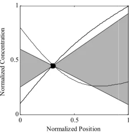
FIGURE 1: POSSIBLE SPACE OF ST
CONCENTRATION PROFILES (SHADED GRAY) FOR SAMPLE DESIRED POSITION AND CONCENTRATIO (BLACK DOT). CURVED BLACK LINES ARE EXAM CONCENTRATION PROFILES THAT CAN BE ACHIE TRANSIENTLY.
Control of DPS is typically achieved by approximating the system to finite-dimensional space with sufficient states to guarantee stability, and then writing a controller for the approximated system [7][8]. One such technique, which has been widely studied in mathematics, is to write
state-space form by defining the state-transition matrix as the Laplacian operator, 2
2
x
A ∂ ∂
= [6]. Related is the orthogonal state projection method, in which the system is projected onto an infinite set of orthogonal basis functions and the calculated using the first N projections [9]. Another approximation involves writing infinite-dimensional transfer functions, expressing them as an infinite sum of partial fraction expansions, and using the first N summations. This has been explained for SISO systems in a recent tutorial publication There also exist non-approximate methods such as boundary control, which maps unstable systems onto stable ones with desired boundary conditions [10].
In all of these methods, the inputs are considered coupled to the PDE measured variable. For example, in considering a system in which chemical diffuse in 1D, an input might be the concentration as some point, z(xin,t), in the diffusion equation
2 2
( , )
( , )
z x t
z x t
D
t
x
∂
∂
=
∂
∂
.The output is also related to the PDE in this way, at so measured position xo, i.e. z(xo,t) or ∂z(xo,t)/∂x.
0 0.5 0 0.5 1 Normalized Position N o rm al iz ed C o n ce n tr at io n
space is infinite dimensional, due to the dependence of dynamics on both position and time [7].
POSSIBLE SPACE OF STEADY-STATE ES (SHADED GRAY) FOR A ION AND CONCENTRATION BLACK LINES ARE EXAMPLE ES THAT CAN BE ACHIEVED
Control of DPS is typically achieved by approximating the dimensional space with sufficient states to guarantee stability, and then writing a controller for the . One such technique, which has been widely studied in mathematics, is to write the PDE in transition matrix as the ated is the orthogonal state projection method, in which the system is projected onto an infinite set of orthogonal basis functions and the calculated . Another approximation dimensional transfer functions, expressing them as an infinite sum of partial fraction summations. This has been explained for SISO systems in a recent tutorial publication [7].
approximate methods such as boundary control, which maps unstable systems onto stable ones with In all of these methods, the inputs are considered coupled riable. For example, in considering a system in which chemical diffuse in 1D, an input might be the
, in the diffusion equation
(1) The output is also related to the PDE in this way, at some
While all these methods can guarantee stability and convergence for many classes of DPS, they are often complex to practically implement and/or require sophisticated mathematics. The infinite dimensi
method mentioned does take a first step in reducing the complexity of this problem, by presenting the system as a transfer function, a form very familiar to students of control theory. Standard software such as MATLAB can be used to design controllers around the approximated systems in the same way they are used for lumped parameter systems. This is, of course, limited to SISO systems, while many DPS have multiple inputs and/or outputs.
We present in this work a method for extendin
dimensional transfer function formulation to MIMO systems by deriving a matrix of transfer functions and transforming this into state-space form. As a case study, we show that we can express a two-input, two-output system governed by Eq. (1 a low order, state-space form and subsequently manipulate the outputs in a simple way by designing controllers using traditional techniques.
MODEL SYSTEM
The motivating system for the problem at hand is a 3 dimensional, microfluidic cell culture assay
the angiogenic response of endothelial cells to a variety of inputs, including chemical factors
focuses on the diffusion of vascular endothelial growth factor (VEGF) specifically, although it can be applied to any other chemical by using the appropriate mass diffusion coefficient,
In the microfluidic device, VEGF diffuses from one flow channel through a porous region, toward the cells and opposing channel, which contains a lower c
Due to the thinness of the device and the assumption that convective transport along the region boundary is fast compared to diffusion across the region, we can model this as a one-dimensional diffusive process
described by Fick’s Second Law of diffusion, given in Equation (1), on the interval 0≤x≤L.
FIGURE 2: SCHEMATIC OF DIFFU
THE CHANNEL CONCENTRATION IS UNIFORM ALO 1
Diffusion H
While all these methods can guarantee stability and convergence for many classes of DPS, they are often complex to practically implement and/or require sophisticated mathematics. The infinite dimensional transfer function method mentioned does take a first step in reducing the complexity of this problem, by presenting the system as a transfer function, a form very familiar to students of control theory. Standard software such as MATLAB can be used to design controllers around the approximated systems in the same way they are used for lumped parameter systems. This is, of course, limited to SISO systems, while many DPS have We present in this work a method for extending the infinite dimensional transfer function formulation to MIMO systems by deriving a matrix of transfer functions and transforming this space form. As a case study, we show that we can output system governed by Eq. (1) in space form and subsequently manipulate the outputs in a simple way by designing controllers using
The motivating system for the problem at hand is a 3-dimensional, microfluidic cell culture assay used for studying the angiogenic response of endothelial cells to a variety of inputs, including chemical factors [11]. This work currently focuses on the diffusion of vascular endothelial growth factor lthough it can be applied to any other chemical by using the appropriate mass diffusion coefficient, D. In the microfluidic device, VEGF diffuses from one flow channel through a porous region, toward the cells and opposing channel, which contains a lower concentration of chemical. Due to the thinness of the device and the assumption that convective transport along the region boundary is fast compared to diffusion across the region, we can model this as a dimensional diffusive process (Figure 2), which is described by Fick’s Second Law of diffusion, given in Equation
: SCHEMATIC OF DIFFUSIVE REGION. H<<L AND ATION IS UNIFORM ALONG W,
W L
SUCH THAT THE DIFFUSION CAN BE ASSUMED TO BE ONE-DIMENSIONAL.
In this system it is of interest to control both the chemical concentration, z(x,t) and the spatial gradient, ∂z(x,t)/∂x, as
cellular behavior is known to be affected by both absolute chemical concentration and the magnitude of a chemical gradient [12]. We propose to control concentration and gradient at a particular point, xo within the diffusive region, such that the outputs are:
1
( )
(
o, )
y t
=
z x t
(2a)2
( )
(
o, )
y t
= ∂
z x t
∂
x
. (2b)Actuation is achieved by specifying the concentration in the microchannels that bound the region, i.e.
1
( )
(
0, )
u t
=
z x
=
t
(3a)2
( )
(
, )
u t
=
z x
=
L t
. (3b) The goal in controlling this two-input, two-output system is to specify both concentration and gradient at a point. Other potential applications include reaching specified concentrations or gradients faster than the typical diffusive time scale, or possibly achieving combinations of concentration and gradient that are not achievable in open loop, although we will focus on the first issue at present.Sensors and Actuators
The proposed hardware for this system incorporates microscopy-based sensing and programmable, on-chip actuation. Microscopy-based sensing is ubiquitous in microfluidics due to the fact that biological assays typically already require microscope data. Furthermore, embedding sensors into microfluidic devices can be difficult and provide limited data, in contrast to the wealth of information present in a single microscope image. For this reason, we consider a CCD camera attached to a fluorescent microscope as our sensor. Provided the chemical of interest is fluorescently tagged, the resulting measurement is an image of the region in which the fluorescence intensity indicates concentration. After calibration and background subtraction, images can be processed in real time to extract the desired outputs: concentration and gradient at any point.
With regards to actuation, we are constrained by the microfluidic device configuration to boundary control only. Assuming no chemical partitioning between the fluid and the gel scaffold, this is implemented via the channels; changing the channel concentration effectively specifies the boundary concentrations. Actuators for this system should accordingly be chosen or designed to both mix certain concentrations of solution upstream of the gel region and deliver this concentration to the gel region boundaries. There exists a wealth of microfluidic actuators to achieve these goals; a number of publications offer a comprehensive review of what
currently exists [14]-[17]. Mixing volumes down to picoliters have been reported, reducing mixing times to milliseconds [16], which is several orders of magnitude smaller than the diffusive time scale (minutes). The proposed plant, then, incorporates both on-chip mixers and pumps, capable of delivering specified concentrations to the boundaries on very short time scales, such that actuator delays need not be modeled.
TRANSFER FUNCTION REPRESENTATION AND APPROXIMATION
To design a controller for a DPS such as the diffusive system just described, it is first necessary to approximate the system in a finite manner. Here, we will do this by first deriving the infinite-dimensional transfer function between each input and each output, as given in Eqs. (2) and (3), then finding a finite approximation for each function by truncating its partial fraction expansion. These approximations can then be assembled into a matrix of transfer functions and converted into state-space form. Finally, standard controllers will be applied to the state-space system to track a given reference.
Deriving Transfer Functions
The method of deriving infinite-dimensional transfer functions is plainly outlined in the tutorial paper by Curtain [7], and will be reiterated only briefly here. The crux of the method is to take the Laplace transform of the PDE with respect to time only, then treat the resulting system as an ODE that contains the Laplace s-variable as a coefficient. For the diffusion equation (Eq. 1), this results in
2 2 ( , ) ( , ) d Z x s sZ x s D dx = , (4)
where the upper-case Z indicates the Laplace transform. Eq. (4) is a second order, linear ODE that is easily solved for Z(x,s)
( )
( )
( , ) sinh s cosh s
D D
Z x s = A x +B x , (5)
with A and B determined by the boundary conditions. As seen in Eqs. (3), the boundary conditions are determined by the choice of input. For the response to input 1, they are
1
(0, )
( )
Z
s
=
U s
(6a)( , )
0
Z L s =
. (6b)Similarly, the boundary conditions when considering input 2 are
(0, )
0
Z
s =
(7a) 2( , )
( )
Z L s
=
U s
. (7b)Substituting Eqs. (6) and (7) into Eq. (5) yields a result of the form
( , )
i( , )
i( )
Z x s
=
f x s U s
(8)for each input i. For inputs delivered at the boundaries only (x=0 or x=L), a linear function between input and output is guaranteed, as either the sinh term will be equal to zero at x=0, as in Eqs. 6, or B is required to be zero by Eq. 7a. Deriving the final transfer function is straightforward from this point; Eq. (8) or its spatial derivative is evaluated at x=xo to produce an equation that includes the output equal to some function times the input. Finally, we divide through by Ui to give each transfer function
( )
( )
j ji iY s
G
U s
=
(9)The resulting four transfer functions are given below:
(
) ( )
(
) ( )
( )
11cosh sinh sinh cosh ( ) sinh s s s s o o D D D D s D x L x L G s L − = (10a)
(
)
( )
12 sinh ( ) sinh s o D s D x G s L = (10b)(
)
(
)
( )
21( ) sinh cosh s D s s o D D G s L x L − = − (10c)(
)
( )
22( ) sinh cosh s D s s o D D G s L x = (10d)Approximating Transfer Functions via Partial Fraction Expansion
Finite dimensional approximations are obtained by first writing the partial fraction expansion of each transfer function, which produces an infinite sum of fractions, and then truncating the summation at some number N. The choice of N is a tradeoff between higher accuracy in the approximation and increased complexity in computation.
To derive the partial fraction expansions, we compute the complex residues for each pole, λn, n=1,2,…,∞, such that each transfer function can be written as
( )
0( )
n n nres
G s
s
λ
λ
∞ ==
−
∑
(11)Mathematically, the residue of any function G(s) at a pole λn is
(
,
n)
lim
(
n)
( )
sres G
s
G s
λλ
λ
→=
−
(12)For a function that can be expressed as the quotient of two functions, G(s) = N(s)/D(s), Eq. (12) simplifies to
(
,
)
(
)
(
)
n n nN
res G
D
λ
λ
λ
=
′
(13)after applying L’Hospitâl’s rule. Using Eq. (13), it is straightforward, however tedious, to develop the partial fraction expansion for each transfer function, by writing out the numerator and first derivative of the denominator for each pole of each transfer function. The poles for all transfer functions (Eqs. 10) are ( ) 2 2 n n L
D
πλ
= −
, and by inspection of the transfer functions, we see that the zeroth order residuals are all zero. This gives us transfer functions, then, that are an infinite sum of partial fraction expansion terms beginning at n=1, which are given for all four functions below:( )
(
)
( )
( )
11 2 2 1 2 sin o n n x L n D G s L s n D π π π ∞ = = +∑
(14a)( )
( )
(
)
( )
( )
1 12 2 2 1 1n 2 sin o n n x L n D G s L s n D π π π + ∞ = − = +∑
(14b)( )
( )
( )
( )
2 2 21 2 2 1 cos n xo D L L n n G s L s n D π π π ∞ = = +∑
(14c)( )
( )
( )
( )
( )
12 2 22 2 2 1 1 n D cos n xo L L n n G s L s n D π π π + ∞ = − = +∑
(14d)Assembling the Approximated State-Space Form
Once the partial fraction expansions are obtained, approximating the system follows easily. As mentioned, the summations of the expansions (Eqs. 14) are truncated at some
n=N, where N is sufficiently large to adequately portray the
system dynamics (other tradeoffs will be noted in later sections). These approximated forms are then assembled into a transfer function matrix:
( )
11( )
( )
12( )
( )
21 22G
s
G
s
G s
G
s
G
s
=
(15) such that( )
( )
( )
( )
( )
1 1 2 2Y s
U
s
G s
Y
s
U
s
=
(16)The transformation from a transfer function (or transfer function matrix) representation to state-space representation can be done computationally (for example, using the ss
function along with the ‘minreal’ property in MATLAB). The resulting state-space representation will have N states, such
that while higher N results in more accuracy, the tradeoff is higher computation requirements. The system takes the familiar form
A
Bu
y
C
χ
χ
χ
=
+
=
ɺ
, (17)for a system modeled without disturbances. In order to avoid confusion with the spatial variable, x, we will refer to the states as χn, n=1,2,…,N.
PROPOSED CONTROLLER DESIGN
With the approximated system described by Eq. (17), traditional state-space controller design techniques can be applied to control the system. The objective of feedback control here is to regulate the concentration and gradient of a single chemical within a one-dimensional diffusion system. This system is inherently stable with no disturbances, meaning that stabilization is not one of aims of this controller. Instead, we focus on improving the speed of response and tracking references. The inputs are an imposed concentration at the endpoints of the region. More rigorously, this can be stated in the following manner:
Given a state-space system governed by the PDE presented in Eq. (1), we wish to create a control law of the form
u
= −
K
χ
+
r
(18) in order to:1. Track references for the outputs y1(t)=z(xo,t) and y2(t)=∂z(xo,t)/∂x.
2. Reach desired concentrations and/or gradients faster than the open-loop, diffusive time scale.
(Note that for the MIMO system at hand, χ,u and r are all
vectors, although we will drop the vector notation for clarity). As the emphasis of this work is on the formulation of the model equations rather than novel controller design, in what follows, we will focus employing well-known techniques in the context of this problem. Tuning the speed of response can be achieved via pole-placement, while steady-state error can be eliminated using integral control. The latter is implemented in state-space systems via the augmented state method, described in many introductory control texts. In this method, an additional state, χI, defined as the integral of the error, is introduced: t I
edt
χ
=
∫
(19a)e
= −
r
y
(19b) such that IC
r
χ
ɺ
= −
χ
+
(19c)Again, for the MIMO system, χI,and e are both vectors. For this augmented system, the gain matrix K is also extended to include both the proportional and integral gains
p e
K
=
K
K
(20) and the resulting state equations are(
)
0
1
0
p e I IA
BK
BK
r
C
χ
χ
χ
χ
−
=
+
−
ɺ
ɺ
(21a)[
0
]
Iy
C
χ
χ
= −
(21b) RESULTSHere we present the results of both the finite-dimensional approximation and the application of basic controllers. As a baseline for comparing the approximations, we use the numerical solution to the 1D diffusion equation (Eq. 1), calculated using the MATLAB PDE solver, pdeval. The geometry for this problem was taken from the example microfluidic device, described in the Model System section, with L=1300µm.
The diffusion coefficient used in simulation was that of Dextran in collagen. Dextran is a fluorescent molecule that can be produced at comparable molecular weight to VEGF (40 kDa for Dextran and 38kDa for VEGF) and is used as a surrogate molecule to simulate the behavior of VEGF. A fluorescent molecule is preferred, particularly in the context of feedback control, as it can be sensed and quantified using standard microscopy techniques. The diffusion coefficient used for Dextran in collagen was 2.7 × 10⁻⁷ cm/s [13].
System Approximation
To verify the accuracy of the approximation, the response of the system to step responses u1(t)=2, u2(t)=1, t>0 was compared against the numerical solution with the appropriate boundary conditions, i.e. z(x=0,t)=2, z(x=L,t)=1. Normalized units of concentration are used throughout, such that z is unitless and ∂z(x,t)/∂x has units µm-1. The simulation was run for xo=600µm. There was good agreement between the approximated systems and the numerical solutions (Figure 3), with accuracy increasing for higher N, as expected.
As a practical check, the step responses of the individual input-output pairs were compared with the corresponding numerical simulations, for both the transfer function and state-space representations. We observed good agreement here as well (results not shown). The model was also verified for other points of interest (xo), shown in Figure 4.
FIGURE 3: APPROXIMATE SYSTEM RESPONSE (SOLID) AND NUMERICAL SOLUTION (DASHED) TO STEP RESPONSE OF U1=2, U2=1 FOR XO=600µM.
FIGURE 4: APPROXIMATED MODEL STEP RESPONSE OF
U1=2, U2=1, FOR (A) XO=100µM (B) XO=400µM (C) XO=600µM
(D) XO=900µM (E) XO=1100µM.
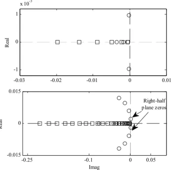
One significant issue with this method of approximation is that it may result in non-minimum phase zeros. As an example, we examine the transfer function between input 1 and output 1, G11 (Eq. 10a). The true zeros of this system are
( )
2o n
n x
z
= −
π (22)which are all on the real axis in the left-half-plane. The zeros of the approximated system, however, can be complex, depending on the polynomial resulting from the approximation. For instance, for N = 6 summations, the zeros are
(
)
3 3 3 1 2 3 3 4 , 5 0.39 10 1.65 10 3.48 10 0.24 0.96 10 , , z z z z i − − − − = − × = − × = − × = − ± × (23)i.e., some complex but all in the left-half-plane. On the other hand, with N = 20, some of the complex poles are in the right-half-plane. These are shown inFigure 5.
FIGURE 5: COMPARISON OF TRUE ZEROS (SQUARES) AND APPROXIMATED ZEROS (CIRCLES). FOR SOME N, THE APPROXIMATION MAY BECOME NON-MINIMUM PHASE. SHOWN FOR N=6 (TOP) AND N=20 (BOTTOM).
Controllers
Controllers based on pole placement and integral control were designed to both speed up the system dynamics and track a reference step input. Using pole placement, on a very low-order approximation (N=2), we were able to manipulate the system dynamics. This is shown in Figure 6 for a step reference r=[1 -0.001], i.e. the desired output is a concentration of 1 and gradient -0.001 µm-1 at xo for t>0. Pole locations were chosen in a fairly ad hoc manner, but as a proof of concept we can see that this is an effective method for manipulating dynamics. However, the steady-state error for the desired concentration is quite high, and the required control efforts take on non-physical values (negative concentrations, Figure 7, top). 0 400 800 0 1 2 C o n ce n tr at io n ( a. u .) Time (min) 0 400 800 -8 -4 0 x 10-4 G ra d ie n t (a .u ./µ m ) Time (min) 0 400 800 0 1 2 C o n ce n tr at io n ( a. u .) Time (min) (a) (b) (e) (d) (c) -0.03 -0.02 -0.01 0 0.01 -1 0 1 x 10⁻³ R ea l -0.25 -0.1 0 0.05 -0.015 0 0.015 Imag R ea l Right-half plane zeros
FIGURE 6: SYSTEM RESPONSE USING POLE PLACEMENT WITH REFERENCE INPUT R=[1,-0.001].
FIGURE 7: CONTROL EFFORTS (TOP), AND ERRORS FOR CONCENTRATION (BOTTOM LEFT) AND GRADIENT (BOTTOM RIGHT), USING POLE PLACEMENT.
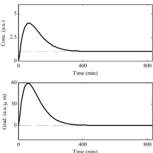
Next, integral control was added via augmented states as previously described. In this way, we were able to achieve zero steady-state error in response to reference step inputs (of the appropriate magnitude and units) for concentration and gradient simultaneously. Figure 8 shows this for the same reference input used previously, and again for N=2. The fact that zero steady-state error can be achieved on this low order approximation is encouraging.
FIGURE 8: RESPONSE TO A STEP REFERENCE OF R=[1,-0.001] USING INTEGRAL CONTROL.
While these results are positive in that they prove that a zero steady state error is achievable in theory, inspection of the control signals again shows that non-physical controls (negative concentrations) are called for (results not shown). Furthermore, as Figure 8 shows, the current controllers may create transient concentrations and gradients that are significantly higher than the desired final concentration, possibly having adverse effects on the cells under study. The need for a more sophisticated control law with input constraints and possibly penalties on the state trajectories is clear.
CONCLUSIONS
Presented in this work was a method for describing a 2-input, 2-output, one-dimensional diffusion process—a distributed parameter system—in a finite manner suitable for control. The outputs considered were chemical concentration and gradient at a particular point in the system, and the inputs were concentrations at the endpoints. Distributed parameter systems exist frequently in control problems and are widely addressed in literature, but controller design for DPS is often highly theoretical in nature and not practical for implementation. Our method, in contrast, expresses the system in a form that classical controllers can easily be applied to.
The method presented here was an extension of the concept of infinite dimensional transfer functions. The finite-dimensional approximation of these transfer functions was developed by expressing them as an infinite series using partial fraction expansion and then truncating the series. For systems that are stable in their full form, the approximation will have a finite error relative to the exact system. This error decreases with increasing summations. A consequence of this approximation, however, is that the zeros of the approximation are not the same as the original system and may even have right-half-plane zeros. Thus, a system that was once minimum
0 400 800 0 .5 1 Time (min) C o n c. ( a. u .) 0 400 800 -6 -4 -2 0 2x 10 -4 Time (min) G ra d . (a .u ./µ m ) 0 400 800 -0.1 0 0.1 Time (min) C o n ce n tr at io n ( a. u .) u 1 u 2 0 400 800 0 0.4 0.8 Time (min) C o n c. e rr o r (a .u .) 0 400 800 -1.2 -0.8 -0.4 0x 10 -3 Time (min) G ra d . E rr o r (a .u ./µ m ) 0 400 800 0 2.5 5 Time (min) C o n c. ( a. u .) 0 400 800 0 30 60 Time (min) G ra d . (a .u ./µ m )
phase may be approximated to a non-minimum phase system. This was seen in Figure 5. While this is not ideal, the appropriate controller can mitigate the effect.
While the primary purpose of this work was to develop a set of state-space equations for the MIMO diffusion system, some preliminary controllers were also developed in order to assess whether these equations were appropriate. Standard techniques such as pole placement and integral control were applied to the approximate state-space system to change the system behavior. It was shown that these techniques were effective on systems with order as low as N=2, a significant computational saving. A drawback to these simple methods is that no provision is made for input constraints or conflicting requirements between the two outputs. Other control methods, in particular optimal control, will be explored in the future. Finally, all of the controllers discussed assumed full state-feedback. This is useful only as an initial check of the utility of the state space system developed; in a true implementation, only the outputs are measurable. Thus, these controllers alone are insufficient for implementing in a real system.
This work presents a novel approach to controlling MIMO distributed parameter systems by extending an infinite transfer function method developed for SISO systems. This method is straightforward to implement in standard computational packages and does not require additional software specific to controller design. In the future, we intend to incorporate these control laws into the hardware platform described, in order to provide specified chemical inputs to a biological assay. With the expansion of biological engineering and the increase in quantitative biological studies, such a tool is an important step in proper experiments for data-driven modeling.
ACKNOWLEDGMENTS
The authors are grateful for the financial support of the Singapore MIT Alliance for Research and Technology, the MIT Martin Fellowship in Design, and the MIT Presidential Fellowship.
REFERENCES
[1] B. Alberts. Molecular biology of the cell, 2008. Volume 1, 5th ed. Garland Science, New York.
[2] F. Lin, W. Saadi, S.W. Rhee, S. Wang, S. Mittal, and N.L. Jeon. 2004. “Generation of dynamic temporal and spatial concentration gradients using microfluidic devices.” Lab
on a Chip, 4 pp.164-167.
[3] H. Song and M. Poo, 1999. “Signal transduction underlying growth cone guidance by diffusible factors.”
Current Opinion in Neurobiology, 9 pp. 355-363.
[4] H. Gerhardt. 2008. VEGF in Development. Springer, New York.
[5] J. Adler and W. Tso. 1974. “Decision-making in bacteria: Chemotactic response of escherichia coli to conflicting stimuli.” Science, 184, pp. 1292-1294.
[6] R. Curtain and H. Zwart, 1995. An Introduction to Infinite-Dimensional Linear Systems Theory. Springer-Verlag, New York.
[7] R. Curtain and K. Morris, 2009. “Transfer function of distributed parameter systems: A tutorial.” Automatica, 45, Jan, pp. 1101-1116.
[8] M.J. Balas, 1979. “Feedback control of linear diffusion processes.” International Journal of Control, 29(3), pp. 523-533.
[9] K. A. Hoo and D. Zheng, 2001. “Low-order control-relevant models for a class of distributed parameter systems.” Chemical Engineering Science, 56, Aug., pp. 6683-6710.
[10] M. Krstic and A. Smyshlyaev, 2008. Boundary Control of PDEs. SIAM, Philadelphia.
[11] S. Chung, R. Sudo, P.J. Mack, C. Wan, V. Vickerman, and R. Kamm. 2009, “Cell migration into scaffolds under co-culture conditions in a microfluidic platform.” Lab on a
Chip, 9 pp. 269-275.
[12] H. Gerhardt, M. Golding, M. Fruttiger, C. Ruhrberg, A. Lundkvist, A. Abramsson, M. Jeltsch, C. Mitchell, K. Alitalo, D. Shima, and C. Betsholtz. 2003. “VEGF guides angiogenic sprouting utilizing endothelial tip cell filopdia.”
Journal of Cell Biology, 161(6), Jun., pp. 1163-1177
[13] S. Ramanujan, A. Pluen, T.D. McKee, E.B. Brown, Y. Boucher, and R.K. Jain. 2002. “Diffusion and convection in collagen gels: implications for transport in the tumor interstitium.” Biophysical Journal, 83(3), Sep., pp. 1650-1660.
[14] B.D. Iverson and S.V. Garimella. 2008. “Recent advances in microscale pumping technologies: a review and evaluation.” Microfluidics and Nanofluidics, 5, Feb., pp. 145-174.
[15] N. Nguyen and Z. Wu. 2005. “Micromixers—a review.”
Journal of Micromechanics and Microengineering, 15,
Dec., pp. R1-R16.
[16] B. He, B.J. Burke, X. Zhang, R. Zhang, and F.E. Regnier. 2001. “A picoliter-volume mixer for microfluidic analytical systems.” Analytical Chemistry, 73(9) May, pp. 1942-1947.
[17] M.A. Unger, H. Chou, T. Thorsen, A. Schere, and S.R. Quake. 2000. “Monolithic micro-fabricated valves and pumps by multilayer soft lithography.” Science, 288 Apr., pp.113-11