Study of reduced kinetic models for plasma turbulence

HAL Id: tel-01898629

https://pastel.archives-ouvertes.fr/tel-01898629

HAL is a multi-disciplinary open access archive for the deposit and dissemination of sci-entific research documents, whether they are pub-lished or not. The documents may come from teaching and research institutions in France or abroad, or from public or private research centers.

L’archive ouverte pluridisciplinaire HAL, est destinée au dépôt et à la diffusion de documents scientifiques de niveau recherche, publiés ou non, émanant des établissements d’enseignement et de recherche français ou étrangers, des laboratoires publics ou privés.

To cite this version:

Shaokang Xu. Study of reduced kinetic models for plasma turbulence. Plasma Physics [physics.plasm-ph]. Université Paris Saclay (COmUE), 2018. English. �NNT : 2018SACLX057�. �tel-01898629�

Study of reduced kinetic models

for plasma turbulence

Thèse de doctorat de l'Université Paris-Saclay

préparée à l’École Polytechnique

École doctorale n°572 Ondes et Matière (EDOM)

Spécialité de doctorat: Physique des Plasmas

Thèse présentée et soutenue à Paris, le 09 Oct 2018, par

Shaokang XU

许 少康

Composition du Jury : Sébastien Galtier

Professeur, LPP, École Polytechnique, Université de Paris-Saclay Président

Étienne Gravier

Professeur, IJL, Université de Lorraine Rapporteur

Johan Anderson

Associate Professor, Chalmers University of Technology Rapporteur

Nicolas Besse

Professeur, Observatoire de la Côte d’Azur Examinateur

Éric Serre

Professeur, Laboratoire M2P2, Aix-Marseille Université Examinateur

Alberto Bottino

Chercheur, Max Planck Institute for Plasma Physics Examinateur

Pascale Hennequin

Directeur de Recherche, LPP, École polytechnique, CNRS Examinateur

Özgür Gürcan

Chercheur (HDR), LPP, École Polytechnique, CNRS Directeur de thèse

Pierre Morel

Maître de Conférence, LPP, Université de Paris-Saclay Co-Directeur de thèse

N

N

T

:

2

0

1

8

S

temps de confinement nécessaire à la réalisation de la fusion thermonucléaire contrôlée. La description de la turbulence cinétique du plasma est un prob-lème à 3 coordonnées spatiales et 3 coordonnées en vitesse.

En se basant sur le fort champ magnétique de confinement, l’approche gy-rocinétique, largement utilisée, consiste à moyenner le mouvement cyclotron, qui est beaucoup plus rapide que le phénomène de turbulence. Une telle réduction permet de simplifier le problème à trois coordonnées spatiales, rel-atives aux centres-guides des particules, une vitesse parallèle ou énergie et une vitesse perpendiculaire apparaissant comme l’invariant adiabatique. La description gyrocinétique non linéaire requiert des simulations numériques de haute performance massivement parallèles. Toute la difficulté est dûe aux termes non linéaires (crochets de Poisson) qui décrivent les interactions multi-échelles, ce qui constitue un défi tant pour la théorie que pour la sim-ulation. Toute approche réduite, basée sur des hypothèses bien contrôlées, est donc intéressante à développer.

Sur la base de cette ambition, cette thèse concerne la turbulence des par-ticules piégées dans le plasma magnétisé : ces parpar-ticules disposent en effet d’une énergie cinétique parallèle insuffisante pour décrire toute une surface magnétique et décrivent un mouvement de rebond côté faible champ magné-tique. En considérant des échelles de temps de la turbulence grandes à la fois devant la fréquence cyclotron et la fréquence de rebond, une double moyenne de la fonction de distribution des particules sur les mouvements cyclotron et de rebond est utilisée, et un système 4D est obtenu qui peut être considéré comme une forme réduite de la théorie gyrocinétique standard. Nous l’avons appelé "bounce averaged gyrokinetics" pendant ce travail. Même si cette description est grandement réduite par rapport à la théorie gyrocinétique, sa simulation numérique directe reste un challenge.

Une description des termes non linéaires en coordonnées polaires est choisie, avec une grille logarithmique en norme du vecteur d’onde, tandis que les angles sont discrétisés sur une grille régulière. L’utilisation d’une grille logarithmique permet de prendre en compte une large gamme de vecteurs d’ondes, donc la physique à très petite échelle. De manière analogue aux modèles en couches en turbulence fluide et afin de simplifier le système, seules les interactions entre couches voisines sont considérées.

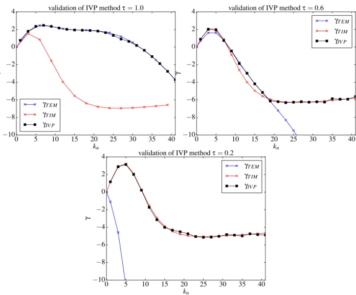
valider les codes numériques non-linéaires vis-à-vis d’un solveur aux valeurs propres développé indépendamment.

Dans un second temps, l’hypothèse d’isotropie dans l’espace de Fourier est utilisée. Ainsi il n’y a pas d’information de phase exacte pour de tels modèles en couches 1D, ce qui laisse un paramètre libre dans les coefficients d’interaction et un choix de phase arbitraire pour les inconnues permettant d’utiliser deux modèles : Gledzer-Ohkitani-Yamada (GOY) et Sabra. Les spectres en nombre d’onde révèlent des lois de puissance originales,

approx-imativement ∝ k−4 pour l’énergie potentielle électrostatique (E

φ), et ∝ k−1

pour l’énergie libre (Ef). Ces exposants ne s’avèrent pas affectés par la valeur

du paramètre libre, mesurant l’intensité des effets non-linéaires relativement aux termes linéaires. La comparaison entre les modèles GOY et Sabra mon-tre de grandes différences quant au niveau de saturation et au comporte-ment temporel de la phase turbulente, en particulier des oscillations à basse fréquence sont obersvées à l’aide du modèle GOY, mais ne sont pas retrouvées dans les simulations basées sur un modèle Sabra.

L’information de phase apparait donc comme très importante. De plus, puisque le taux de croissance d’instabilité est anisotrope, la simulation du modèle anisotrope doit être réalisée dans un troisième temps. Le système résolu numériquement est réduit à une espèce cinétique, en supposant que les autres espèces sont adiabatiques. Deux systèmes différents peuvent ainsi être étudiés : ions cinétiques et électrons adiabatiques (IC) d’une part, ou électrons cinétiques et ions adiabatiques (EC) d’autre part. Les spectres en nombre d’onde de l’énergie potentielle électrostatique et de l’entropie

mon-trent des exposants similaires dans les deux cas : ∝ k−5 pour l’énergie

po-tentielle électrostatique et ∝ k−7/3 pour l’énergie libre. Par ailleurs, dans

le cas d’électrons cinétiques une dynamique de type prédateur-proie entre le flux zonal et la turbulence est observée, où le flux zonal présente une oscil-lation forte et régulière. Il faut noter que le niveau de flux zonaux dans le système avec ions cinétiques est significativement plus elevé que dans le cas d’électrons cinétiques.

Enfin, un système complètement cinétique (CC) est étudié. La compara-ison avec les deux systèmes (IC) et (EC) montre des différences significatives

cas d’électrons cinétiques avec ions adiabatiques (EC) en ce qui concerne le mécanisme de saturation : le maximum du spectre est observé glisser pro-gressivement du maximum de taux de croissance linéaire (avec k ≈ 20) vers des nombres d’ondes plus faibles (typiquement k ≈ 3). En même temps, l’anisotropie du spectre observée dans le cas (IC) est retrouvée dans le cas (CC), avec un rôle important joué par les streamers (modes correspondant à des tourbillons allongés radialement). Ceci interroge sur la pertinence de l’approximation d’une réponse adiabatique que ce soit pour les ions ou, plus communément effectuée, pour les électrons.

1 Introduction: turbulence and transport in Tokamaks 10

1.1 Nuclear fusion . . . 10

1.1.1 Nuclear fusion reaction . . . 10

1.1.2 Lawson criterion . . . 11

1.2 Kinetic description of plasma turbulence . . . 14

1.2.1 Vlasov equation . . . 15

1.2.2 Quasi-neutrality equation . . . 15

1.2.3 Difficulty of nonlinear simulation . . . 15

1.3 Reduced model . . . 16

1.3.1 Trapped particle model . . . 16

1.3.2 Simplifications in fluid turbulence . . . 17

2 Bounce averaged gyrokineticsδ f equations in Fourier space. 20 2.1 Introduction . . . 20

2.2 Bounce averaged gyrokinetics . . . 21

2.2.1 Model equations . . . 21

2.2.2 Scale separation . . . 24

2.2.3 Normalization . . . 25

2.3 δf equations in Fourier space . . . 27

2.4 Description of nonlinear interactions . . . 28

2.4.1 Description of k+p+q = 0 . . . 29

2.4.2 Description of the nonlinear terms . . . 31

2.4.3 Different approaches and connections to previous models . . . 33

2.4.4 Conserved quantities. . . 35

2.5 Conclusion . . . 36

3 Linear Phase 38 3.1 Linear dispersion relation . . . 38

3.1.1 Plasma dielectric function: ǫ(ω) . . . 39

3.1.2 Singularity and residue . . . 40

3.2 Threshold of the temperature gradient driven instability . . . 40

3.2.1 Threshold of κT and the wave number k . . . 42

3.2.2 Threshold of κT and ion to electron temperature ratio τ . . . 43

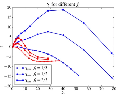
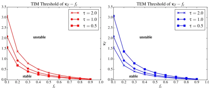
3.2.3 Threshold of κT and the trapped particle ratio ft . . . 44

3.3 Linear instability . . . 44

3.3.1 Numerical method: argument principle . . . 45

3.3.2 Linear instability for isotropy system: γ(k) with k = kα= kψ . . . 48

3.3.3 Linear instability for anisotropic system: γ¡kψ, kα ¢ . . . 49

3.4 Conclusion . . . 53

4 Isotropic model: Sabra and GOY 54 4.1 Model equations . . . 55

4.1.1 Phase approximation . . . 55

4.1.2 Model equations . . . 56

4.2 Nonlinear simulation of the Sabra model . . . 58

4.2.1 Code verification . . . 58

4.2.2 k spectra of the electrostatic potential energy Eφ . . . 60

4.2.3 k spectra of the entropy Ef and kinetic effect . . . 63

4.2.4 The effect of free parameter α . . . 63

4.3 Influence of phase information: GOY vs Sabra . . . 64

4.3.1 Oscillatory dynamics of the GOY Model . . . 65

4.3.2 Comparison of entropy . . . 67

4.3.3 Oscillation of the k-spectra . . . 68

4.4 Conclusion . . . 69

5 Anisotropic model: LDM 71 5.1 LDM of bounce averaged gyrokinetics . . . 71

5.1.1 LDM Grid . . . 71

5.1.2 Vlasov-Poisson equation . . . 71

5.1.3 Numerical scheme . . . 74

5.1.4 Definition of zonal flow and dissipation . . . 75

5.2 Kinetic ions . . . 77

5.2.1 Temporal spectrum of Eφand Efi . . . 77

5.2.2 Spectrum of electrostatic potential Eφin wave number plane . . . 78

5.2.3 k spectra of Eφand Efi . . . 78

5.3 Kinetic electrons . . . 79

5.3.1 Temporal spectrum of Eφand Efe . . . 79

5.3.2 Predator-prey dynamics between zonal flow and turbulence modes . . . 80

5.3.3 Spectrum of Eφin wave number plane . . . 82

5.3.4 k spectra of electrostatic potential energy Eφand entropy Efe . . . 83

5.4 Fully kinetic system . . . 84

5.4.1 Temporal spectrum of Eφ, Efi and Efe . . . 85

5.4.2 Spectrum of Eφin wave number plane . . . 85

5.4.3 k spectra of Eφ, Efi and Efe . . . 86

5.4.4 Comparison of the k-spectra: adiabaticity . . . 87

6 Conclusion and perspective 92

A Calculating the coefficients of GOY model 96

B The linear dispersion relation solver 100

B.1 Linear dispersion relation ǫ(ω) . . . 100 B.2 Eigenvalue solver . . . 102

C Formulation of gyro correction 105

D Comparison of J0sand its approximations 108

E Electrostatic potential energy Eφand entropy Efs 112

Tokamaks

Energy is the most important issue in modern society. As a consequence of the development of civilization, the worldwide demand for energy has been increasing rapidly. In most of the countries around the world, energy is produced mainly by fossil fuels, even though many new sources and techniques exist. As a resource that can not be reproduced, the fossil fuels stored in the earth is fixed, which will certainly reach the end one day in the future, especially when the growth of world population is considered. Another big problem that is more urgent, is the pol-lution and the greenhouse effect, caused by the combustion of fossil fuels, which endanger the health of everyone, including the planet earth. So the research of new energy sources, especially those that are clean and abundant, is becoming more and more important.

1.1 Nuclear fusion

1.1.1 Nuclear fusion reaction

One of the possibilities, inspired by the reaction in the stars, is the transformation of fusion energy to electric energy, which has been envisaged at least from 50s. The method is to confine the light nuclides such as deuterium (D), tritium (T ), helium-3 (He3), and lithium (Li ) as shown in figure (1.1), by a strong magnetic field in a reactor like Tokamak such that the nuclides can produce energy in the process of fusion reactions:

D + T → α(3.5Mev) + n (14.1Mev) D + D → T (1.01Mev) + p (3.03Mev) D + D → He3(0.82Mev) + n (2.45Mev) D + He3→ α(3.67Mev) + p (14.67Mev) Li6_{+ n → T + α + 4.8Mev} Li7_{+ n → T + α + n − 2.5Mev ,} (1.1) 10

Figure 1.1: Binding energy per nucleon[2].

Since the energy is produced by nuclear reactions, the greenhouse effect that is linked spe-cially to fossil fuels, is not an issue. Deuterium exists abundantly in sea water with an amount that could supply the energy consumption for more than millions of years, while tritium can be “breeded” using lithium, another abundant element. Furthermore fusion reactions do not leave long lasting radioactive products, and the problem of nuclear waste is much less serious than that for fission reactors.

The energy produced in this reaction is so high that the power of the designed fusion reactor, for example 500 Mw for ITER (International Thermonuclear Experimental Reactor), is usually very high comparing to that of the other power station in the world. If one day the nuclear fusion becomes a reality, energy will not be a limit for human beings for a long time.

1.1.2 Lawson criterion

The binding energy per nucleon is relatively small in very light or very heavy nuclides, as shown in figure (1.1)[2][40], while heavy nuclides provide the fuel for fission reactors, the lighter ones (which have especially low binding energy, such as H, D and T ) provide the potential fuel for fusion. The difficulty in extracting this energy is that, in order to achieve fusion reaction, one has to supply enough energy to heat the plasma to temperatures, which will allow positively charged particles to overcome their repulsive Coulomb potentials with a sufficient rate so that fusion reactions can occur. For example the reaction rate of one deuterium due to a large number of tritium atoms is given by:

d N

Figure 1.2: Fusion cross section as a function of the kinetic energy for different reactions [2]. where N is the number of reaction and d N

d t is the reaction rate, nT is the number of tritium per

volume, σ is the cross section and v is the relative velocity between the particles, the average 〈·〉 is performed on the velocity distribution of the particles. There are many possible fusion reactions, however D − T reaction has the largest cross section as shown in figure (1.2) [1] and the released energy is also the largest among the reactions given in equation (1.1), which is the main reason to choose the deuterium and tritium as the fuel in modern fusion reactor like the ITER machine.

In the case of many particles, one can obtain the reaction rate as follows:

d N

d t = nDnT〈σv〉 ,

thus the total fusion power Pfusionshould be :

Pfusion= d Et ot d t =d(N Efusion) d t = nDnT〈σv〉Efusion,

where Et ot is the total fusion energy, which is the sum of the energy Efusion produced in each

fusion reaction. In order to understand the power budget, the fusion power should be compared to the power loss from the plasma, for which one can introduce the confinement time τE, such

that: dWt h d t = − Wt h τE + Pl ,

where Pl is the loss of power, which can be seen as the sum of the radiation power of α particles

defined as Pa= Pf us_EαE_+Eα_n and the external power Pext supplied to heat the plasma. Wt his the

thermal energy of plasma, which can be written as:

Wt h≈ µ3 2nDTD+ 3 2nTTT+ 3 2neTe ¶ V ≈ 3neTeV ,

with the assumption of a D − T mixture such that nD = nT =n₂e. In stationary regime, the

con-finement time can be defined as the ratio of the plasma thermal energy to the loss of power[40]:

τE=

Wt h

Pl

.

The confinement time can be understood as the period τE for which the plasma is confined.

Another key parameter of a fusion reactor is the amplification factor of the plasma Q , which is defined as:

Q =Pf us Pext

.

If Q = ∞, the reaction is self sustained by the fusion power, which is called ignition. If Q = 1, it is called “break-even”, since one gets as much power from the device as one puts in.

An important and general criterion to measure the system to be able to produce energy, is that the generated fusion power should be able to maintain the temperature of the plasma against the loss of power without external power input such that the temperature is high enough to heat the plasma and to continue the fusion reaction[15]:

Pf us> Pl ,

which, after a detailed calculation, gives a minimum required value for the product of the plasma (electron) density ne , the temperature of the plasma T (10 ∼ 20 kev) and the energy

confine-ment time τE, called the Lawson criterion [34]. For the system of deuterium and tritium, it

neTτE > 3 ∗ 1021kev.m−3.s .

This relation gives two different ways of fusion: the inertial fusion, which works with a very short confinement time (τE ∼ 10−11s) and a very high density (n ∼ 1031m−3) and the magnetic

confinement fusion, where the density is reduced to n ∼ 1020m−3and the confinement time is τE ∼ 1s.

In the magnetic confinement fusion, the temperature of the system should be high enough (~15 kev ) to continue the reaction. The density of the plasma ne is limited by the parameter

β = pki n

pmag of the plasma with pki n, the kinetic pressure of the plasma defined as pki n= nekT and

pmag, the magnetic pressure of the plasma defined as pmag = B

2

2µ0, where B is the magnetic field

and µ is the magnetic moment. The plasma β parameter must be smaller than 1 such that the magnetic pressure is higher than the kinetic pressure to avoid the disruption of the plasma.

Due to these conditions, the choice of the plasma density ne and the temperature T is

lim-ited, to satisfy Lawson criterion, it is necessary to make the energy confinement time τE as long

as possible. However the confinement of the particle and the heat in the Tokamak is not stable, due to the diffusive transport of the density, as well as the heat from the center to the boundary of machine, which can be formulated as:

∂tn = D△n ,

∂tT = χ△T ,

with n and T , the density and the temperature, D and χ the diffusion coefficients of density and heat, respectively. This diffusive transport is what limits the confinement and strongly depends on the level of turbulence energy. So the control of turbulent transport is one of the key require-ments for the improvement of the energy confinement time to make fusion energy a reality.

1.2 Kinetic description of plasma turbulence

In order to control the turbulent transport in a Tokamak, it is necessary to understand the mech-anism of the turbulence and transport of the magnetized plasma. The understanding of the tur-bulence and transport in a Tokamak is mainly via the description of the temporal behavior of the plasma. A plasma consist of many ions and electrons, but the individual behavior of each particle can hardly be observed. What can be observed instead are statistical average, thus it is necessary to define a distribution function in the phase space to describe the evolution of a plasma. Note that if the density of a plasma is very low, it is seen as a collection of individual particles. If the density as well as the collision rate are high enough, it is seen as a fluid, between these two cases, it is seen as a kinetic plasma. The distribution function of a kinetic plasma can be introduced as f (r, v, t), where r and v present the particle positions and the velocities, respectively.

1.2.1 Vlasov equation

The evolution of the particle distribution function f (r, v, t) is described by the Vlasov equation, that is:

∂ f ∂t −

£

H , f¤_{r,v= 0 ,} (1.2)

with H , the Hamiltonian of the particles, which can be generally defined as H ≡_2m1_s¡P− qsA

¢2

+

qsΦ, with P, the canonical momentum; A, the magnetic vector potential; Φ, the electric

po-tential; ms and qs, the mass and the charge of the particle, respectively.

£

H , f¤is the Poisson bracket defined as£H , f¤₌d H_{d r} d f_{d v−}d f_{d r} d H_{d v} . The right hand side of this formula is 0 for a colli-sionless plasma. Note that the particle distribution function f of a kinetic plasma depends on 3 spatial coordinates and 3 kinetic coordinates (or velocity). So it is a 6D system.

1.2.2 Quasi-neutrality equation

Vlasov equation is coupled to the electromagnetic fields, described by Maxwell’s equations. When magnetic fluctuations are small as that observed in a tokamak and for scales that are larger than Debye length λD, the system can be seen as quasi-neutral, which means the

fluctu-ation of ion density δni should be equal to the fluctuation of electron density δne:

δni= δne, (1.3)

where the density δns, can be calculated by the integration of the particle distribution function

fs over the kinetic coordinates, where the index s = i, e represents the species of interest.

1.2.3 Difficulty of nonlinear simulation

A 6D problem is a challenge for theoretical analysis, so the understanding of this high dimen-sional system is based mainly on numerical simulations. Considering the capability of today’s computers, simplification is useful for this system. One possible technique is to average out the cyclotron motion, since the cyclotron frequency ωc of the charged particle in a strong magnetic

field is much higher than the typical frequency of plasma turbulence. This widely used tech-nique, the so called gyro average[8] in the field of gyrokinetic simulations, can reduce the 3D velocity coordinate to 2D, since the phase information of the cyclotron motion is averaged out:

¡

v_||, v_⊥,θ¢=⇒¡v_||, v_⊥¢ ,

where v_||is the velocity that is parallel to the magnetic field, v_⊥is the perpendicular velocity and

θ is the phase of the cyclotron motion. After the gyro average (figure(1.3)), the 6D kinetic

Figure 1.3: The 6D phase space is reduced to 5D by gyro average, where the phase of cyclotron motion is lost[18].

parallel velocity or energy and one perpendicular velocity appearing as the adiabatic invariant, the cyclotron phase is lost in gyro average).

Nonlinear gyrokinetic[5, 18] simulations are usually massively parallel high performance nu-merical simulations. Note that being a 5D problem, the computation of nonlinear dynamics in gyrokinetic description that includes self-consistent multi-scale interactions usually requires millions of CPU hours and makes anything beyond medium nonlinear runs dominated by a sin-gle type of instability over a small range of scales, impractical. This, coupled with the complex-ity of numerical implementation can also make it harder to understand and isolate important physical mechanisms. In this regard, reduced models appear as intermediate tools, that are use-ful for isolating important physical mechanisms, to provide guidance to large scale gyrokinetic simulation efforts as well as comparison with experiments.

1.3 Reduced model

Caused by the complexity and the difficulty of the nonlinear gyrokinetic simulation, reduced models are potentially very promising.

1.3.1 Trapped particle model

Gyro average allows to reduce the 6D kinetic system to a 5D gyrokinetic system. Considering the motion of a charged particle, further simplification is possible. In a magnetic configuration of a Tokamak, where the magnetic field is stronger on the inner side than on the outer side, a charged particle can be trapped or passing depending on its kinetic energy due to the mirror effect. So in addition to the cyclotron motion, it displays also the bounce motion and the toroidal precession motion. Since the cyclotron frequency ωc and the bounce frequency ωb are much higher than

the toroidal precession motion ωp, it allows to average out the cyclotron motion as well as the

bounce motion as shown in figure(1.4):

This double average (gyro average plus bounce average) is called gyro bounce average[18, 16], which is usually used to simplify the discussion of the trapped particle (i.e, Trapped Electron

Figure 1.4: The motion of a charged particle in a Tokamak, due to the gradient of the magnetic field, a charged particle can be passing (right upper figure) or trapped (right lower figure) de-pending on its kinetic energy. The left upper figure shows the parallel motion of the passing particle and the left lower figure shows the bounce motion and the toroidal precession motion of the trapped particle[18].

Mode (TEM) and Trapped Ion Mode (TIM)) [31, 9, 50] turbulence and results in a 4D system[16, 14] (i.e. two spatial coordinates: the toroidal angle α and the poloidal flux ψ playing the role of radial coordinate r , and two kinetic parameters: particle energy E and an adiabatic invariant µ appearing as the trappeed particle ratio ft ):

f ⇒ f ¡α, ψ(r ),E ,µ¢.

Note that the gyro average reduces the 3D kinetic coordinates to 2D and the bounce average reduces, in some sense, the 3D spatial coordinates to 2D. So this is a 2D kinetic system, which is used to describe the TEM and TIM turbulence in the toroidal plane of a Tokamak. This 4D model is initially developed by IJL (Institut Jean Lamour) of Lorraine University [16, 14, 20, 21, 15] in collaboration with CEA IRFM Cadarache as a reduced form of the 5D gyrokinetic model [17]. A quick and detailed introduction of this model is given in chapter 2 section 2.2.

1.3.2 Simplifications in fluid turbulence

Even though the trapped particle model is much simpler than 5D gyrokinetics, the 4D simula-tion is still expensive, especially if a wide range of scales are to be considered, due to the nonlin-ear nature of this model. Thus, further simplifications, especially on the nonlinnonlin-ear interactions, without losing any essential features of the initial model is useful.

The study of kinetic plasma turbulence is relatively new, however turbulence is everywhere in nature and its study dates back to ancient Greeks, yet important developments have been made in this field over the years. In plasmas, there exist a number of descriptions, from the full Klimontovich description to simple reduced fluid models such as Hasegawa-Mima[29], or Hasegawa-Wakatani equations[28]. Furthermore, different variants of reduced fluid models such as MHD[48, 22], reduced MHD, Hall MHD etc. have been studied into details in the context of solar wind turbulence, and of the solar dynamo problem.

Inspired by previous works, especially the description of nonlinear effects in fluid turbu-lence, a kinetic reduced form of trapped particle model has been worked out during this thesis. Different from the generic gyrokinetic simulation in real space, the method here is to resolve the kinetic Vlasov-Poisson system in Fourier space, where the Poisson bracket becomes a convolu-tion after the Fourier transform. The convoluconvolu-tion is associated to a constraint on the wave vec-tors: k+p+q=0, which means that the evolution of mode k is determined by the mode p and the mode q such that p+q=-k. Note that this standard constraint gives rise to the so called nonlinear multiscale interactions, which is also the most challenging part of the turbulence problem: all the difficulty and complexity comes from this term.

A promising technique used in fluid turbulence is the logarithmic discretization for the wave number k:

k = kn= k0gn,

where k0is a free parameter, g > 1 is the logarithmic spacing factor and n is the shell number.

This method allows to consider a very large range of scales in numerical simulations, which is practically impossible for the gyrokinetic simulation in real space.

In order to run the simulation, an analytic expression of the nonlinear terms should be given. Note that in general the relation of the wave vector k+p+q = 0 corresponds exactly to a triangle. Based on the existence condition of a triangle, which is principally determined by the moduli of the wave vector (i.e. wave number), a selection of all the possible triads in a given range of wave numbers has been worked out, which allows a full description of the nonlinear terms based on the triad information. In practice only a subset of all the possible interactions is taken into account in simulation, to simplify the nonlinear expression and to save time. For example the popular subset of the local interactions that is used in GOY[43] or Sabra models[37]:

{n − 2 ,n − 1 ,n ,n + 1 ,n + 2},

which means that the nonlinear interactions are between the nearest neighboring modes. Simu-lation presents that the logarithmical discretization of the wave number space and the assump-tion of local interacassump-tions are rather efficient and some important results have been found based on this method, which is comparable to the direct nonlinear simulation in real space.

The aims of this thesis is to give a detailed and analytical formulation of the nonlinear mul-tiscale interactions by using previous methods that exist in fluid or MHD turbulence problems and then apply these new nonlinear descriptions to the 4D trapped particle turbulence model.

Even though kinetic plasma turbulence is different from the fluid turbulence, the nonlinear de-scription here doesn’t destroy the kinetic effects, for example toroidal precession resonance is well observed in these simulations.

Moreover, inspired by the logarithmically discretized model (LDM)[25], which has been de-veloped to resolve the 2D passive scalar equation, a further description of the nonlinear terms respecting the conservation of entropy and electrostatic potential energy has been worked out in a 2D polar coordinates based on the triad condition. This description is more general and complete, where different approaches connected to the previous models like GOY, LDM, etc can be found: it can be seen as a development of the previous ones.

This report is organized as follows: in chapter II the trapped particle model is introduced quickly, as well as the Fourier transformation of the model equations. An analytic expression of the nonlinear terms as well as their connections to the previous models has been presented too. Chapter III is contributed to discuss the linear phase of the system, such as the linear disper-sion relation, the threshold of parameters and the linear instability. A numerical method based on the argument principle has been developed to resolve the linear dispersion relation, where singularity and multi roots co-exist. In chapter IV and chapter V the nonlinear simulation is presented for the isotropic model and the anisotropic model, respectively. A conclusion and a perspective is given in chapter VI as the last chapter.

in Fourier space.

2.1 Introduction

Nonlinearity is the most challenging aspect of kinetic plasma turbulence, yet in order to make fusion a reality, it is necessary to understand the nonlinear mechanisms of the turbulent phe-nomena in fusion reactor. Our ambition in this thesis is to try some new methods to represent the nonlinearity of the kinetic plasma turbulence, since direct nonlinear simulations of the 5D gyrokinetic system is expensive. This kind of large simulation is largely impractical for the study of multi-scale physics for most of the usual laboratories or institutes, which, as a consequence, limits the understanding of this problem.

Inspired by previous efforts to treat the nonlinearity in fluid turbulence, for example the Hasegawa-Wakatani model[28], the simple shell models such as GOY[43], Sabra[35], as well as the more advanced and recently developed 2D LDM[25] and the 3D Nested polyhedra model of turbulence [22] etc, a new description of the nonlinear kinetic plasma turbulence will be built to interpret the multiscale interaction between the particle distribution function and the elec-trostatic potential fluctuations. As a first step, this description will be applied to the trapped particle turbulence [31, 9, 50] model, which, as a reduction of the standard 5D gyrokinetics[5], provides a simple testbed.

Plasma turbulence is usually more complicated than the fluid turbulence, because in addi-tion to the spatial phenomenon, the kinetic effects, such as the kinetic resonance, is also con-tained in kinetic plasma turbulence. Note that this work does not do any simplification on the kinetic aspects of plasma turbulence, so all the models beyond this work are totally kinetic even though we use ideas of fluid turbulence.

This chapter is organized as follows: in section (2.2) the trapped particle model[11, 16], or as it is more generally called bounce averaged gyrokinetics, will be introduced, where we will detail the Vlasov equation, the quasineutrality equation as well as the normalization of this model. In section (2.3) we will develop a formulation to describe the nonlinear terms of the bounce aver-aged gyrokinetic model in a special log polar coordinate system. This new developed formula-tion is able to describe all the nonlinear couplings in a very large range of scales as well as handle

anisotropy and it can be applied to other turbulence problems even though we begin with the trapped particle model. Since the formulation developed here contains all the nonlinear cou-plings, different reduced models can be found based on different assumptions, which shows a clear connection to the reduced models of fluid turbulence. The conservation of the quadratic quantities, such as the electrostatic potential energy and the entropy, is demonstrated in section (2.4). Note that the conservation laws, as an essential nonlinear property of the Poisson bracket must be valid by our models.

2.2 Bounce averaged gyrokinetics

The bounce averaged gyrokinetics model[11, 16] is initially developed by the Institute of Jean Lamour (IJL) in University of Lorraine, in collaboration with IRFM (Institut de Recherche sur la Fusion par confinement Magnetique) in CEA Cadarache, as a reduced form of the 5D gyroki-netics system, to study the TEM and TIM turbulence in Tokamak [16, 14, 20, 21]. In addition to the gyro average operator that is widely used in gyrokinetics, the bounce average operator is also used in this model to further simplify the system, which finally results in a 4D (i.e. 2 spatial coordinates + 2 kinetic coordinates ) kinetic plasma turbulence model.

2.2.1 Model equations

A full description of a kinetic ion-electron plasma requires solving the 6D Vlasov equation for electrons and ions, which can be given in the action-angle coordinates (Ji,αi) as follows:

∂ fs ∂t − £ H , fs ¤ αi, Ji = 0 , (2.1)

where fs is the full particle distribution function corresponding to species s (i.e. s = i, for

ions, s = e for electrons), and H is the Hamiltonian, which can be generally defined as H ≡

1 2ms

¡

P− qsA

¢2

+qsΦ, with P, the canonical momentum; A, the magnetic vector potential; Φ, the

electric potential; msand qs, the mass and the charge of the particle, respectively.

£

H , f¤_αi,Ji is the Poisson bracket defined as:

£ H , f¤_α i,Ji ≡ X i ½_∂H ∂αi ∂ f ∂Ji − ∂H ∂Ji ∂ f ∂αi ¾ , (2.2)

where αi and Ji correspond respectively to the angles (or phases) and actions associated to the

cyclotron motion (i = 1), the bounce motion (i = 2) and the toroidal precession motion (i = 3), which are defined as[16]:

J =    J1= −m_qs_sµ J2= ¸ m_2πsvg ∥d s J3= msR vg ∥+ qsψ    α =   α1= ωct + cnt α_{2= ωbt + cnt} α3= ωdt + cnt   (2.3)

Table 2.1: Standard spatial and temporal parameters of ions and electrons for the ITER machine[15].

where µ is the usual adiabatic invariant defined as µ ≡ msv2_⊥

2B with v⊥, the perpendicular

veloc-ity, v_{g ∥}is the parallel velocity of the guiding center. ωc, ωb and ωd correspond respectively to

the frequencies of cyclotron motion, bounce motion and toroidal precession motion. ψ is the poloidal flux and stands for the radial coordinate since dψ = −R0Bθd r . Note that the action

variables Jican be considered as adiabatic invariants because the variation of the actions Jiare

much slower than the time scales of the periodic movements. In this case the action variables Ji

can be seen as conserved during the movement:

d Ji d t = − ∂H ∂αi = 0 , dαi d t = ∂H ∂Ji = ωi . (2.4)

This spatial, temporal and kinetic system is 6 + 1D and is equivalent to a description in real space and velocity space Vlasov equation:

fs= fs(t,α1,α2,α3, J1, J2, J3) . (2.5)

Considering the motion of particles, allows further simplification. Since in a standard toka-mak configuration, for example the standard parameters of ions and electrons for the ITER ma-chine as shown in table(2.1), the cyclotron frequency ωcand the bounce frequency ωbare much

higher than the toroidal precession frequency ωd (i.e. (ωc, ωb) ≫ ωd), it is possible to average

the Vlasov equation over both the cyclotron motion and the bounce motion, if we are interested mainly by time scale of the toroidal precession motion, which is also the characteristic time scale of the TEM/TIM turbulence[16]. This double average is called gyro bounce average in the following. Comparing to the general gyro average, the average over the bounce motion is also taken into account, which results in a 4D system, since the phase information of both the cy-clotron motion and the bounce motion are averaged out. This means that when we perform the double average, we can write:

f (t,α1,α2,α3, J1, J2, J3) ⇒ ¯f(t,α3, J1, J2, J3) . (2.6)

Inserting the definitions of the action variables in equation (2.3), the distribution function can be represented with the usual variables:

¯f(t,α3, J1, J2, J3) ⇒ ¯f¡t ,α, µ, E , ψ¢ , (2.7)

here α = α3 is the toroidal precession angle, µ is the adiabatic invariant associated with the

action of cyclotron motion J1, E is the particle energy associated with the action of bounce

motion J2 and ψ is the poloidal flux associated with the action of precession motion J3. The

resulting Vlasov equation after this double average, depends only on 2 variables (precession an-gle α and poloidal flux ψ, which plays the role of the radial coordinate r in this configuration.), parametrized by the particle energy E and the adiabatic invariant µ, which gives 2 spatial coor-dinates and 2 coorcoor-dinates in velocity space, and thus a complete problem in 4D.

Considering the dynamics of each motion in the case of electrostatic fluctuations, the Hamil-tonian H of the particle can be given as follows:

H _{= J}3Ωd+ qsφ + ... , (2.8)

where J3Ωd is the kinetic energy connected to the toroidal precession motion with Ωd, the

pre-cession frequency of the particle. qsφ is the electrostatic potential energy with φ, the

electro-static potential. There should be other potentials associated to the bounce motion and the cy-clotron motion, however after the gyro bounce average, these potentials will not pass to the fur-ther calculation, so they are not detailed here. Substituting the Hamiltonian into Vlasov equa-tion and after some manipulaequa-tions, it results in[16, 14]:

∂ f_s ∂t − h J0sφ, fs i α,ψ+ EΩd Zs ∂ f_s ∂α = 0 , (2.9)

where f_s are the full (equilibrium and fluctuation) particle distribution functions associated with the species s that are averaged over bounce and cyclotron motions. ΩdE /Zsis the toroidal

precession frequency of a particle with the energy E and the atomic number Zs. J0sis the gyro

bounce average operator (which will be defined in Fourier space in the next section). Note that in the calculation of equation (2.9) we use d H

dαi = 0 and

d H d J1,2= 0 .

2.2.2 Scale separation

It is common to make an assumption of scale separation between background profiles and small scale fluctuations that make up the turbulence in Tokamaks. Considering the scale separation between the equilibrium and the fluctuations, one can write the bounce center distribution function as:

f_s¡E ,µ, α, ψ, t¢_{= F}s¡E ,µ, ψ¢+ δf_s¡E ,µ, α, ψ, t¢. (2.10)

where Fs is the equilibrium distribution function of the species s, which, in this model, is

as-sumed to be Maxwellian and independent of time:

Fs ¡ E ,µ, ψ¢₌neq,s ¡ ψ¢ T_eq,s1.5 ¡ψ¢ e −µB + 1 2 ms v∥2 Teq,s _{. (2.11)}

Inserting this definition into the Vlasov equation, one can obtain the equation of the fluctu-ating part δfs: ∂δ f_s ∂t − ∂J0sφ ∂α ∂Fs ∂ψ + EΩd Zs ∂δ f_s ∂α − h J0sφ, δ fs i α,ψ= 0 . (2.12)

Note that this is the Vlasov δfs equation of the bounce averaged gyrokinetics model. In

or-der to close the system, this equation is coupled to Maxwell equations with self-generated and imposed fields, which in the case of electrostatic fluctuations with no externally applied electric fields becomes the quasi-neutrality equation:

δni= δne, (2.13)

for scales that are larger than the Debye length. In tokamak geometry, a charged particle can be either “passing” or “trapped” in the low field side depending on its kinetics energy, as shown in figure(1.4), so the density of the particle can be seen as the sum of two parts:

δns= δnt+ δnp , (2.14)

where δntis the density of the trapped particles, with the index t standing for “trapped”, and δnp

is the density of the passing particles, with the index p standing for “passing”. For the trapped particles, dynamics is kept kinetic, which can be obtained from the integration of the particle distribution function over the velocity coordinates:

δnt =

ˆ

qsJ0sδ fs

p

E d E dµ . (2.15)

Note that the integration with respect to the adiabatic invariant µ gives the trapped particle ratio ft, which should be between 0 and 1. Only one value of ft is passed to simulation, such

that this 4D system can be simplified further to 3D. The correction of the gyro bounce aver-age should also be considered (the difference of the real density and the density of the bounce center), which means:

δnt= ft ·ˆ qsJ0sδ fs p E d E −qs Ts ˆ ¡ 1 − J0s2 ¢ φFs p E d E ¸ . (2.16)

The details of the gyro correction can be found in appendix C.

If the ratio of the trapped particle is ft, then the ratio of the passing particle is 1− ft. In order

to simplify the system, the passing particles are assumed to be adiabatic in this model, which means: δnp= −¡1 − ft¢ q s £ φ − ǫφ ­ φ®_α¤ Ts , (2.17)

where φ − ǫφ< φ >αis due to the response from zonal flow and ǫφdefines this response, which

takes values between 0 and 1 for the zonal modes and is zero for the other modes, because zonal flows have no direct influence on them. Inserting all the ingredients into the density equation, the final quasineutrality equation can be written as follows:

2 p π 1 Te a R0 ˆ · Fe ¡ 1 − J0e2 ¢ φ +1 τFi ¡ 1 − J0i2 ¢ φ¸pE d E +(1 − ft)n0 ftTe a R0 ·µ 1 +1 τ ¶ φ −³ǫe,φ+ ǫi ,φ τ ´­ φ®_α ¸ =p2 π ˆ £ J0ifi− J0efe ¤p E d E . (2.18)

where τ is the ion to electron temperature ratio defined as τ = Ti

Te. ǫi ,φand ǫe,φdefine respectively

the response from zonal flow for ions and electrons. In order to simplify, we use qi = 1 and

qe= −1 respectively for the charge of ions and electrons.

Note that the primary focus of this thesis is the development and the discussion of the re-duced nonlinear descriptions, so we do not discuss the derivation of this model in great detail, we recommend the interested readers to find the details in [16] .

2.2.3 Normalization

It is important to provide proper normalization in order to identify spatial and temporal scales associated with the phenomena that can be studied in bounce averaged gyrokinetics. Here the energy is normalized by a temperature T0, which in this thesis refers to the ion temperature Ti:

ˆ

E = E

The time is normalized by a frequency ω0typically in the time scale of the toroidal precession

motion:

ω0= T0

eR₀2Bθ

, (2.20)

with R0, the major radius of the Tokamak and Bθ, the strength of the poloidal magnetic field.

This frequency represents the ionic frequency of the toroidal precession motion with the tem-perature T0, such that:

ˆt = ω0t . (2.21)

Note that this frequency is also the characteristic frequency of the TIM turbulence. The distance is normalized by a scale defined as:

Lψ= a |

dψ

d r |= aR0Bθ, (2.22)

with a, the minor radius of the Tokamak. This length can be seen as the radial scale of the problem:

ˆ

ψ = ψ Lψ

. (2.23)

Since the poloidal flux plays the role of radial coordinate: ψ = ψ(r ). The electrostatic poten-tial is normalized by ω0Lψ: ˆ Φ = Φ ω0Lψ= R0 a eφ T0 . (2.24)

The particle distribution function fsis normalized as follows:

ˆf = fs n0s ³_2πT 0s ms ´₋3 2 . (2.25)

The bounce averaged gyrokinetics model after these normalizations can be written as fol-lows: ∂ fi ∂t − ∂J0iφ ∂α ∂Fi ¡ ψ¢ ∂ψ + EΩd Zi ∂ fi ∂α− £ J0iφ, fi¤_α,ψ= 0 , ∂ fe ∂t − ∂J0eφ ∂α ∂Fe ¡ ψ¢ ∂ψ − EΩd Ze ∂ fe ∂α− £ J0eφ, fe ¤ α,ψ= 0 . (2.26)

cnφ =

ˆ _¡

J0ifi− J0efe

¢p

E d E . (2.27)

In this equation and from here on, we use fs instead of δfs to simplify the notation. Here,

the prefactor cnin the quasi-neutrality relation is defined as:

cn= a R0 1 Ti ˆ _£ 1 − J0i2 ¤ e−EpE d E + a R0 1 Te ˆ _£ 1 − J0e2 ¤ e−EpE d E + p π 2 (τ + 1) a R0 (1 − ft) ft ¡ 1 − ǫφ ¢ , (2.28)

which is the sum of the polarization (i.e. gyro bounce correction) and the adiabatic response (i.e. passing particle contribution).

2.3

δ f equations in Fourier space

The nonlinear gyrokinetics is the domain of massively parallel high performance numerical sim-ulations through the computation of nonlinear dynamics within a description, which includes self-consistent multi-scale interactions. It usually requires millions of CPU hours and makes anything beyond medium nonlinear runs dominated by a single type of instability over a small range of scales, impractical. As a result of the complexity of numerical implementation, some-times it is hard to understand and isolate important physical mechanisms. In this regard, re-duced models appear as intermediate tools, that are necessary for isolating important physical mechanisms, to provide guidance to large scale gyrokinetic simulation efforts as well as com-parison with experiments.

Based on these ambitions, the following reduced model, which stands on the simplifica-tion of the nonlinear dynamics, without losing any essential features, has been worked out for the trapped particle turbulence model. In this thesis the simulation is implemented in Fourier space, which means:

fs¡α, ψ, µ, E¢=

X k

f_ks¡µ, E¢ei kαα+i kψψ_{, (2.29)}

Inserting this definition into the Vlasov equation, one can obtain the Vlasov equation in the wave numbers plane k=¡kψ, kα

¢ as follows: ∂ f_ks ∂t − i kαJ0sφk ∂Fs ∂ψ + EΩd Zs i kαf_ks − X k+p+q=0 ¡ pψqα− pαqψ ¢ J0sφ∗pfq∗s= 0 . (2.30)

The last term of equation (2.30) is the convolution, which corresponds to the Fourier trans-form of the Poisson bracket. It means that the evolution of the mode k is determined by the mode p and the mode q that should satisfy the wave vector constraint p + q + k = 0. This con-straint defines the nonlinear interactions across scales in turbulence, which presents infinite possibilities and thus a challenge for both theory and simulation.

Nonlinear interactions among scales has been discussed since the beginning in the context of fluid turbulence[29], as well as in MHD turbulence[48]. Various reduced models that describe these scale by scale interactions have been proposed such as the shell models or LDM, or Nested polyhedra model[22]. Inspired by these previous ideas, a reduced representation of the convo-lution will be given based on the description of the wave vector constraint.

Another important point in above equation is the double average operator J0s. In real

space, the bounce average, as well as the gyroaverage, correspond to operators acting on the unknowns, and the double averaging procedure has been symbolized in equation (2.9) by J0sφ.

In Fourier space, the bounce-average and gyro-average can be obtained as simple zeroth or-der Bessel function of the first kind, so that the total average, symbolized by J0sfor the sake of

simplicity in equations (2.18, 2.30), is given by the following product: J0s≡ J0(kψδs0

p

E ) J0(kαρs0

p

E ) . (2.31)

In order to simplify the simulation, different approximations of the average operator has been used based on different scales in previous works [14, 49]. In appendix D we will discuss the difference between the exact average operator and its different approximations, especially the validation of its approximations in very small scales.

2.4 Description of nonlinear interactions

In theory, if the medium is infinite, the wave vector k is a continuum quantity, so in the Fourier plane there are infinite number of waves and in the absence of quantization due to boundary conditions, the number of triads defined by k+p+q = 0 is also infinite, which results in an infinite number of nonlinear interactions. The nonlinearity is the most complicated part in turbulence and analytic solution for such a problem is probably impossible.

However in numerical simulation, the wave vector should be discretized in a cartesian or polar coordinate, linearly or logarithmically, and the number of waves is not infinite. For a given range of discretized waves, the number of interacting triads is fixed, which can be found out easily by a program based on the conditions fixed by the wave vector constraint: k+p+q = 0. The triad information then can be written in a table as a coupling card. Based on this coupling card, it is possible to give an analytic expression of the nonlinear terms. Of course even with an analytic expression, the system is still very complicated and it is difficult to find a solution by theoretical analysis, due to the average operator (Bessel function) and the integration over the kinetic coordinates, etc, but it can be resolved numerically.

In order to give an analytic expression of the nonlinear terms, it is necessary to start from the coupling information defined by the wave vector constraint: k+p+q = 0.

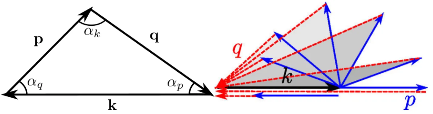
Figure 2.1: k + p + q = 0 in a plane, which in fact forms a triangle with sides of length k, p and q and angles of αk, αp and αq, respectively, as shown by the left figure. The right figure shows the

existence conditions of a triangle: the maximum of (k, p, q) should be smaller or equal to the sum of the two smaller ones; the minimum of (k, p, q) should be larger or equal to the difference of the two larger ones.

2.4.1 Description of k+p+q = 0

The wave vector constraint k+p+q = 0 is very common in fluid turbulence[28, 25], kinetic plasma turbulence[52], as well as in MHD[48]. A detaileddescription of the Poisson bracket in Fourier space ( i.e. equation (2.30)) will be given in this section. The vectors are presented in polar co-ordinates, which means the wave vector k is defined as k = (k, θk), with k, the modulus of the

wave and θk, its orientation. In this coordinate system kαand kψcan be expressed as:

kα= ksin(θk) ,

kψ= kcos(θk) . (2.32)

So k =¡kψ, kα

¢

forms a cartesian coordinate and k = (k, θk) forms a polar coordinate one.

The nonlinear terms can be represented in vector form, independent of components as follows: X p+q+k=0 £ pψqα− pαqψ¤J0sφ∗pfs,q∗ = X p+q+k=0 ¡ ˆz × p¢· qJ0sφ∗pfs,q∗ , (2.33) where p =¡p,θp ¢ and q =¡q,θq ¢

. ˆz is the direction that is perpendicular to the wave number plane k, where¡kψ, kα, ˆz

¢

forms a 3D cartesian coordinate. The wave vector constraint p + q + k = 0 in the Fourier plane is shown in figure(2.1), which in fact describes triangles, with the sides of length k, p and q and angles αk, αpand αq, respectively. The interaction coefficient is defined

as Mkpq= ¡

ˆz × p¢· q , which can be calculated as:

M_{kpq= ˆz ·}¡_{p × q}¢_{= pq sin}¡θp− θq

¢

. (2.34)

The absolute value of the interaction coefficient Mkpq equals the surface of the triangle formed by k, p and q. In reduced models, like GOY, Sabra and LDM, only local interactions (i.e.

however a more important and concrete reason for this is that the surface of the triad formed by neighboring waves is maximum, which, as a reduced model, can qualitatively represent the maximum nonlinearity.

Another important situation is the disparate scale interaction[24][47], where p ∼ k and q ∼ 0. This nonlinear interaction represents the direct transfer between the large scale modes, like the zonal flow (q = 0) and the small scale modes, which is another important mechanism in turbulence.

Note that Mkpq and Mkqp is different due to their opposite sign, as will be shown later that the opposite sign is very important to satisfy the conservation laws.

In general, the constraint p + q + k = 0 defines a triangle. In order to compose a triangle, the moduli (or length) of the vectors should satisfy some constraints as shown in figure(2.1), which are:

i) the sum of any two edges must be larger than (or equal to, in the limit case) the third one. ii) the difference of any two edges must be smaller than (or equal to, in the limit case) the third one.

These two criteria are the necessary and sufficient conditions to determine the existence (or not) of a triangle if the lengths of the three sides are given. Based on these criteria, it is possible to select all the couples¡p, q¢that can interact with the wave number k for a given range of wave

numbers. Note that the selection process acts only on the wave moduli k, p and q. In a triangle, if the three sides are given, the angles can be fixed by the law of the cosines, then this triangle is fixed, which in fact means the phase information is fixed.

The phase information θp and θq of the wave p and q can be obtained from the wave k by

the following relations ( see figure(2.1)):

θp = π + θk+ αq ,

θq= π + θk− αp , (2.35)

here π + θk means the inverse direction of the wave k, αp (αq) is the angle between the wave q

(p) and -k (see figure(2.1)), which can be calculated by the cosines relation of a triangle:

αq= arccos µ q2_{− p}2_{− k}2 2pk ¶ , αp= arccos µ p2_{− q}2_{− k}2 2qk ¶ . (2.36)

From equation (2.35), we can obtain θp−θq= αq+αp, since αp+αq+αk= π, so θp−θq= π−

αk, which will be used in the calculation of interaction coefficients Mkpq. Finally the information of the waves k, p, q as well as the interaction coefficient Mkpqin a polar coordinate are given as follows:

k = (k,θk) , p =¡p ,_{π + θ}k+ αq ¢ , q =¡q ,_{π + θ}k− αp ¢ , Mkpq= pq sin(π − αk) . (2.37)

In order to know the coupling information of a triad, we should have¡k, p, αp, q, αq, Mkpq ¢

, or at least the wave numbers ¡k, p, q¢, since the other elements, such as the phase and the

interaction coefficients can be calculated simply from the wave numbers.

2.4.2 Description of the nonlinear terms

When the coupling information is known, a description of the nonlinear terms can be written. A formulation of Poisson bracket in Fourier space will be laid out in this section based on the definition of the triad.

Considering the permutation of p and q (i.e. φpfq↔φqfp, because the evolution of fk can be determined by φpand fq, it can be also determined by φq and fp), one can write (i.e., see figure(2.2)) the nonlinear terms as:

¡

ˆz × p¢· qJ0sφ∗pfs,q∗ = MkpqJ0sφ∗pfs,q∗ + MkqpJ0sφ∗qfs,p∗ .

(2.38) Considering the vectors that are mirror symmetric with respect to the vector k, for example the reflection vector p′_(q′_{) of p (q) with respect to k , as shown in figure(2.2), is:}

p =¡p ,_{π + θ}k+ αq ¢ k ←→ p′= ¡ p ,_{π + θ}k− αq ¢ , q =¡q ,_{π + θ}k− αp ¢ k ←→ q′= ¡ q ,_{π + θ}k+ αp ¢ . (2.39)

This allows us to write the nonlinear term as: ¡

ˆz × p¢· qJ0sφ∗pfs,q∗ =MkpqJ0sφ∗pfs,q∗ + MkqpJ0sφ∗qfs,p∗

+ Mkp′_q′J0sφ∗_p′fs,q∗′+ Mkq′_p′J0sφ∗_q′fs,p∗ ′. (2.40)

Note that this expression gives a full description of the nonlinear terms for one triad¡k, p, q¢

in the wave plane, which includes the permutation and the reflection of the wave vectors with respect to k, and there are no other possibilities for the same triangle.

From the definition of Mkpqand the relation between the wave vectors p, q and p′and q′, we have the following relations:

k p q α_k α_p α_q Φ_p f_q f_p p q k α_k α_p α_q Φ_q α_q α_k k α_p f_q Φ_p f_p Φ_q α_q p q α_k k αp permutation mirror reflection q p

Figure 2.2: Expansion of the nonlinear terms (Poisson bracket) in the wave number plane by the permutation (right vs left) and the reflection with respect to k(up vs bottom)

Mkpq= − Mkqp,

Mkpq= − Mkp′_q′. (2.41)

Inserting the definitions of the waves p,q,p′_,q′_{and the interaction coefficients into equation}

(2.40), the nonlinear terms of one triad in polar coordinate can be represented as: ¡ ˆz × p¢· qφ∗phq∗= pq sin(π − αk) (φ∗π+θp k+αqh∗π+θ k−αp q − φ∗π+θ k−αp q h∗π+θ k+αq p −φ∗π+θp k−αqh∗π+θ k+αp q + φ∗π+θ k+αp q h∗π+θ k−αq p ) , (2.42)

With these, the Vlasov equation can be expressed in polar coordinates as follows:

∂ fs,k ∂t =i kαJ0sφk ∂Fs ∂ψ − EΩd Zs i kαfs,k + X k(p, q) pq sin_{(π − α}k) ³ φθ_pk+αqh_qθk−αp_{− φ}θ_qk−αphθ_pk+αq_{− φ}θ_pk−αqhθ_qk+αp_{+ φ}θ_qk+αphθ_pk−αq´, (2.43)

here k¡p, q¢means all the couples¡p, q¢that can interact with the mode k . So the nonlinear terms should be the sum of all the possible couplings, which is represented byPin equation (2.43). pq sin(π − αk) is the interaction coefficient of the corresponding triad. Note that this

expression gives a full description of the Fourier transform of 2D Poisson bracket in polar co-ordinates, which includes all (not only a subset of ) the possible couplings (i.e. local couplings, disparate scale couplings and other types) in a given scale. Before doing the simulation, one needs to find out all the couples k¡p, q¢that gives the coupling card of system. After having the coupling card, the Vlasov equation can be simulated directly.

2.4.3 Different approaches and connections to previous models

In the previous section, a description of the nonlinear terms (i.e. Fourier transform of the Pois-son bracket) is worked out in the wave number plane. In simulation, the wave numbers k, p, q can be linear, logarithmic or even random, which is not a limit in this description. However in practice, one must consider the capacity (i.e. memory, threads,etc) of the machine and the in-tention of the research. For example if the nonlinear physics in small scale is of interest, it may be necessary to use logarithmic discretization of the wave number magnitudes, to describe a large range of scales easily. The number of the couplings in logarithmic discretization is much less than that in linear discretization, which will take less time and consume less computer re-sources to run the simulation. This was the main motivation for the development of ”shell mod-els”.

Logarithmic discretization means that the wave number k is discretized as:

k = kn= k0gn, (2.44)

where k0is a free parameter that defines the smallest wave numbers and g > 1 is the logarithmic

scaling factor and n is the shell number.

Equation (2.43) gives a full expression of the Poisson bracket in polar coordinates. Based on this expression, different reduced models can be derived, which are connected to the previous models developed in fluid turbulence.

If only local interactions are considered, for example the widely used reduction:

{(n − 2, n − 1, n),(n − 1, n, n + 1),(n, n + 1, n + 2)} , (2.45) where there are only three coupling triads in nonlinear interactions, the Vlasov equation can be reduced to the form:

∂ f_s,nj ∂t = i kαJ0sφ j n ∂Fs ∂ψ− EΩd Zs i kαfs,nj +1₂k2_ng−4pµ0 h J0sφ∗j +r_n−20f_s,n−1∗j −s0− J0sφ∗j −s_n−10f_s,n−2∗j +r0+ J0sφ∗j +s_n−10f_s,n−2∗j −r0− J0sφ∗j −r_n−20f_s,n−1∗j +s0 i +1₂k2_ng−2pµ0 h J0sφ∗j +l_n−10f_s,n+1∗j −s0− J0sφ∗j −s_n+10f_s,n−1∗j +l0+ J0sφ∗j +s_n+10f_s,n−1∗j −l0− J0sφ∗j −l_n−10f_s,n+1∗j +s0 i +1₂k2_npµ0 h J0sφ∗j +l_n+10f_s,n+2∗j −r0− J0sφ∗j −r_n+20f_s,n+1∗j +l0+ J0sφ∗j +r_n+20f_s,n+1∗j −l0− J0sφ∗j −l_n+10f_s,n+2∗j +r0 i . (2.46) This has the same nonlinear form as the LDM[25], which has been recently developed to resolve the 2D passive scalar equations in fluid turbulence. In this model the wave vector is defined as k =¡kn,θj¢with kn, logarithmically discretized and θj, linearly discretized as θj =

j ∗2π_M, which means that the unit circle in wave number space is divided into M regular sections here. n is the index of the shell number and j is the index of the angle, which should be an integer between 1 and M.

In equation (2.46) r0, l0and s0are the coupling angles (or rather integer index offsets that

correspond to these angles) originated from αp and αq, which should be normalized by 2π_M in

simulation. Note that the coupling angles gives the exact phase information of this 2D cascade model.

Since the particle distribution function f as well as the electrostatic potential φ are real phys-ical quantities, their Fourier components should satisfy the following relations:

f-k= f_k∗,

φ-k= φ∗_k, (2.47)

which allows to simulate the system only in the upper half wave plane [0; π] in Fourier space, the quantities in the other half plane [π; 2π] can be obtained automatically from equation (2.47). The nonlinear simulation of this model will be presented in chapter (V).

Considering the isotropic fluctuations such that kα = kψ, the 2D anisotropic turbulence

problem can be simplified to a 1D problem. In this case the phase information θj is lost and

one has the freedom to choose different phase approximations. Note that the fact that there is no exact phase information, is a general problem in 1D shell models. Shell models also have a free parameter α in the nonlinear interaction coefficients. Since the model becomes 1D , the coupling angles r0, l0 ,s0, etc, of this model will be 0 or π, depending on different phase

ap-proximation, which finally results in different models. For example if we use the well known GOY version phase approximation, the isotropic cascade model [24, 52] of the bounce averaged gyrokinetics can be written as follows: