Labelling Operators

(1)

HAL Id: hal-01134346

https://hal.archives-ouvertes.fr/hal-01134346

Preprint submitted on 23 Mar 2015

HAL is a multi-disciplinary open access archive for the deposit and dissemination of sci-entific research documents, whether they are pub-lished or not. The documents may come from teaching and research institutions in France or abroad, or from public or private research centers.

L’archive ouverte pluridisciplinaire HAL, est destinée au dépôt et à la diffusion de documents scientifiques de niveau recherche, publiés ou non, émanant des établissements d’enseignement et de recherche français ou étrangers, des laboratoires publics ou privés.

Labelling Operators

Serge Beucher

To cite this version:

(2)

Labelling Operators

(Programming tricks with MAMBA)

Serge BEUCHER

CMM/ARMINES/Mines ParisTech June 2014

1. Introduction

The MAMBA image library is basically a mathematical morphology library which contains a large number of efficient and fast morphological operators. Some of them have been implemented in C (the watershed transform, the geodesic reconstruction, a very efficient particle labelling operator and obviously all the basic neighboring operators used to build more and more sophisticated ones). However, many of them are implemented in Python. Compared to C, Python brings more flexibility even if a slight reduction of the performance may be awaited. Nevertheless, very fast and efficient transforms, as erosions and dilations or filters with large structuring elements, can efficiently be designed in Python.

In some cases, however, specific operators are needed. Implementing them in Python requires then some hints to design sufficiently performing algorithms. Operators involving connected components or region labelling are particularly important to design filters based on criteria or attributes or in the definition of residual transforms.

This note describes implementations in MAMBA of some particle or region labellings. These operators are used to quickly label each connected component of an image with the result of a measure applied on it. A typical example of this kind of operator is the area opening where each particle of a set is given the value of its area (refer to the MAMBA examples on the Web site) but the implementation is more general and can be used with other measures.

Other labelling techniques will also be described. They are based on the use of distance functions associated with reconstructions of the connected components of a binary image or the cells of a partition image. Here again, an example of this kind of approach can be found with the labelling of connected components with their Feret diameter (also in the MAMBA examples). These algorithms mainly use various tricks to cope with the slowness of operators performing individual analysis of particles. The extension of these operators to grey tone images (that is to the cells of a partition formed by an image) will also be described. To achieve this, the operators defined on partitions and described in [1] are used.

Note that no really new morphological operator is introduced in this paper. Its purpose is simply to explain some programming tricks which have been used to design specific operators which are not available in the MAMBA library but nevertheless which can be realized by means of a clever use of some fast MAMBA transformations.

(3)

We shall start our descriptions in the binary case. Then, in the second part, the algorithms will be extended to partitions.

2. labelling binary sets

Two main labelling techniques will be addressed. The first one consists in labelling each connected component with the number of some specific points which are included in the connected component. This approach is used, in particular, in the labelling of sets by their stereological measures. The second technique is based on the propagation of a specific pixel value inside each connected component. This second approach obviously uses various geodesic reconstructions.

2.1. Labelling with stereological measures

In this section, we describe how to label each connected component of a set with a value equal to one of its stereological (or Minkowski) measures. Although it is possible, as said above, to achieve this labelling particle by particle, the implementation described here is much more efficient as 255 particles can be processed in parallel.

As explained in another document [2] describing how stereological measures are implemented in MAMBA, a measure is always performed in two steps: a transformation which detects some specific points in the set followed by a simple counting of these points. In 2D, three measures are defined:

- The area where the transformation is the identity (we simply count the number of pixels in each connected component).

- The diameter (or diametral variation) in a given direction where the operator used is a Hit-or-Miss Transformation (HMT) by a doublet of points oriented in the selected direction. Note that the perimeter of each particle can be obtained, up to a constant, by averaging the diametral variations in all directions according to the Cauchy-Crofton formula [3].

- Obtaining the connectivity number is a little bit more complicated as it requires the use of two or three HMT transforms. Remind that, in 2D, the connectivity number is equal, for each connected component, to one minus its number of holes. Therefore, in order to avoid negative or zero labels which are not very handy, another measure will be used: 1 + nH, where nH is the number of holes. This measure is always positive and we can write:

✚=₁−_nH where ν is the connectivity number.

Then:

1+nH=2−✚

These labellings are achieved by using the classical labelling operator of a set which assigns to each connected component a single integer value, followed by the computation of grey tone histograms and the use of look-up tables. The histogram operator (getHistogram in MAMBA) computes, for each grey value, the number of pixels which are assigned this grey value in the image. The look-up operator (lookup in MAMBA) allows to replace each grey

(4)

value of an image by another value stored in a look-up table. These operators are implemented efficiently in MAMBA. They are fast as they require a single scan of the image.

2.1.1. Area labelling

Let us describe this implementation in the case of the labelling of each connected component by its area.

Let X be a binary set made of n connected components Xi. The labelling operator assigns to each Xi a single value i thus producing a label function f:

f(x)=i if x c Xi

(background point) f(x)=0 if x " X

When computing the histogram of f, each entry i of the histogram contains a value h(i) which is equal to the area ai of Xi because this connected component is the only one where its pixels are assigned the grey value i. Therefore, the histogram table can be used as a look-up table to replace the previous grey value i inside each connected component Xi of X by a new value equal to its area ai.

The practical implementation of the procedure is a bit more complex for two reasons. The first one comes from the fact that both histogram computation and look-up procedure can only be applied on greyscale images (8-bit, 256 grey levels). As a set X may contain more than 255 connected components (the background is always labelled with 0), it is not possible to process all of them at the same time. The second reason is due to the value of the area of the connected components which may be higher than 255. Therefore, it is not possible to use directly this value in the look-up operator. In order to cope with these two problems, firstly, only 255 particles are processed at the same time. Thus, the computing speed is reduced. However, the process remains 255 times faster than a classical implementation based on individual analysis. Secondly, the area value ai of each particle Xi is decomposed into four values, a_i0, a_i1, _a and according to the following formula:

i 2 _a i 3 ai=

✟

j=0 3 a_ij.256j

Each being less than 256, it can be used in a look-up table. So, four look-up tables l0, l1, l2a_ij and l3 are defined, each one being applied to the corresponding byte plane of the final label image f’. We have:

ai=h(i)

Then ai is decomposed into four values (a_i0, _a , , ) according to the above formula. Each i 1 _a i 2 _a i 3

is loaded in the corresponding look-up table: a_ij

lj(i)=a_ij

Finally, at each point x of the image, the value of the new label image f’ is given by: f∏(x)=

✟

j=0 3

lj(f(x)).256j

Once the first 255 particles have been processed, the 255 following ones are extracted (by subtracting 255 to the initial label image, then by extracting the least significant byte plane and by keeping the labels between 0 and 255) and processed. The computation stops when all the particles have been processed.

(5)

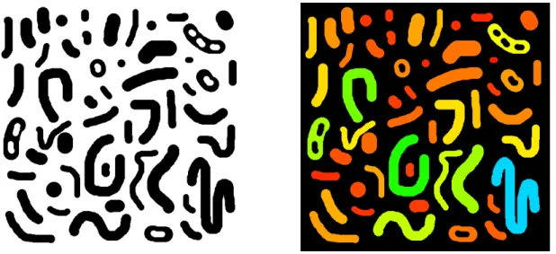
The MAMBA implementation of this algorithm, called areaLabelling, is given in annex. As already mentioned above, this procedure has been used in a MAMBA example (see exampleA17.py) to perform an area opening of a set. Figure 1 shows this area labelling applied on a set of bubbles.

Figure 1: Labelling of bubbles with their area (note that the label values, in all the figures, have been normalized in order to be contained in the range [0,255 ] for an easier display).

2.1.2. Stereological measure labelling

The same algorithm can be used to label particles with their stereological measures as diametral variations, perimeters and connectivity numbers.

Let us see how it works with the diameter in the horizontal direction. We know that this measure is equal, for each connected component, up to a scalar factor (which will be dicarded in the labelling) to the number of (01) configurations (also called intercepts) in the component [2]. Therefore, labelling each component with its diameter is straightforward and performed in two steps:

- Detection of all the (01) configurations in the image (with a HMT transform where the origin of the structuring elements is put on the 1-pixel in order to be sure that the detected points fall inside X).

- Infimum of the previous set with the original labelled image and application of the previously described procedure to this new labelled image.

We see immediately that for each particle labelled with the value i, only intercept points corresponding to this particle will receive the same label in the new image. Therefore the histogram calculation and the look-up tables will replace this initial value i by the diameter value.

To achieve this, a general transform called measureLabelling (see the annex) is designed. It takes two input images, the image of the particles to be labelled and the image containing the pixels to be counted to obtain the measure. This procedure is almost identical to the areaLabelling one. We just added a new input image containing the pixels obtained by the measure transformation and the infimum of this image and the initial label image.

(6)

The diameterLabelling procedure provides the general implementation of this labelling by diameters (Figure 2).

Figure 2: Labelling particles with their horizontal diametral variations.

Labelling each connected component with its number of holes nH (or more precisely, as explained above, with nH + 1) is a little bit more complex. However, it still uses the measureLabelling procedure. Let us explain this on the hexagonal grid. We know that the connectivity number (Euler-Poincaré constant) of a 2D set is given by:✚

✚=_N 0 0

1 −N

0

1 1

that is the difference of the number of occurrence of these two triangular configurations. These configurations can be extracted by means of appropriate HMT transforms.

The number of holes of each particle Xi, nH (Xi) is equal to: nH(Xi)=1−✚_i where is the connectivity number of the particle Xi.✚_i

Figure 3: Labelling particles with their number of holes +1. The purple particle is labelled with value 485. Its connectivity number is equal to -483. This connected component contains 484 holes.

(7)

We want to label this particle with the value 1+nH(Xi)=2−✚_i. To do this, we can define two label images l1 and l2. l1 contains as labels the number of 0 0 configurations in

1

each particle of the initial image and l2 the number of 0 configurations (once again,

1 1

take care of choosing the origin of the HMT structuring elements among the 1-pixels). Then, the final label image l containing the value 1+nH(Xi) for each particle Xi is given by:

l=2+l2−l1 This function is always strictly positive inside the particles.

Figure 3 gives an example of the use of the procedure named holesLabelling. 2.2. Labelling with other measures

It is possible to label connected components of a set X with other measures. This can be done by using the geodesic reconstruction which propagates in the entire connected component a value which has been determined by a specific procedure.

2.2.1. Labelling with the Feret diameter

A typical example of this kind of labelling is the (horizontal or vertical) Feret diameter labelling. This example is also given in the MAMBA examples (see exampleA20.py). Let us explain how it is performed for the horizontal Feret diameter.

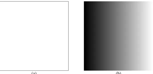
Consider an image with a width equal to w and a height equal to h. The first step of the procedure consists in generating a distance function d which will be equal, for each pixel of coordinates (x, y) of the image, to d(x, y) = x + 1. This distance function can be obtained easily and rapidly by generating a binary set filling all the image except a vertical line at the left side (Figure 4a) and by computing the distance function of this set (with computeDistance). Then, we add 1 to this image (Figure 4b).

Figure 4: The distance function (b) of the binary image (a) is used as a template in the set labelling with the Feret diameter.

(b) (a)

(8)

The second step consists in performing the infimum between this distance function and the indicator function of the original image X (this indicator function takes the maximum value for each point belonging to X). We obtain then a new function where, in each connected component, its maximal value is equal to 1 + the largest x-coordinate of all the vertical lines cutting this component. If we perform a geodesic reconstruction of the indicator function with this distance function, each connected component will be labelled with a value equal to this maximal x-coordinate + 1. Let us denote l1 this label image. Conversely, if we perform a dual geodesic reconstruction, we obtain another label image l2 containing for each connected component the lowest x-coordinate of all the vertical lines cutting this component. We can get the label image l corresponding to the horizontal Feret diameter by:

l=l1−l2+1

A similar operator can be defined for the vertical Feret diameter (Figure 5). This operator named feretDiameterLabelling is described in the annex.

Figure 5: Example of Feret horizontal and vertical diameters labellings. 2.2.2. Labelling with volumes

Another interesting procedure consists in labelling connected components of a set X with the volume of the restriction of a function f inside each connected component of X. Let X be a set and f a function with positive integer values. We have:

X=

4

i Xi each Xi being a connected component of X.

We can measure the volume vi of the function f inside each connected component Xi: vi =

¶

Xi

f(x)dx The function f can be decomposed in the following way:

f(x)=

✟

k=0 n−1

ak(x)2k

with ak(x) c [0, 1] and n the number of bits in the decomposition. Then, we have:

¶

Xi f(x)dx=

¶

Xi

✟

k=0 n−1 ak(x)2k_dx=

_✟

k=0 n−1

¶

Xi ak(x)2k_dx=

_✟

k=0 n−1 2k

_¶

Xi ak(x)dx

(9)

For a given value k,

¶

is equal to the area of the intersection of Xi with the bit plane k Xi

ak(x)dx of f.

Once again, the measureLabelling procedure can be used to achieve this volume labelling. The following algorithm can be designed If f is defined with n bits, we have:

Initialize the final label image l with 0. For k = 0 to (n-1), do:

Extract the k-th bit plane Zk of f

Label X with the area of the intersection Zk3 X . Let lk be the label function Let l = l + 2k_lk

Figure 6: The lower catchment basins of the initial image (a) are extracted (b), in red (minima in yellow. Their volume (c) is used in their labelling (d).

(d) (c)

(b) (a)

(10)

This labelling can be used in various operations: volume-controlled watershed transform, labelling of the contours of a segmentation by the average value of the gradient on each contour, for instance.

This procedure, called volumeLabelling, is defined in the annex.

Figure 6 illustrates the use of this operator for the labelling of lower catchment basins with their volume.

3. Labelling partitions

The same operators can be defined on partitions as they are defined in [1] instead of binary connected components provided that each cell of the partition is assigned a single and unique label value. In this case, labelling each cell with the number of points which fall inside it is made by means of the same algorithm as the one presented above: all the points falling in one cell are given the label of the cell and their number is obtained by the histogram. The new labelling is performed by the look-up table defined by the histogram.

However, when a partition corresponds to the different flat zones of a function according to the general definition given in [1], this approach does not work as different cells may have the same label. Therefore, on this kind of partition, a new labelling must be performed where each cell is assigned a single and unique label value. Unfortunately, this procedure does not exist in the current MAMBA release (it will likely be added in a future one).

3.1. General partition labelling

It is, nevertheless, possible to design a procedure for labelling general partitions. This procedure uses a special image together with the reconstruction operators available in the partition.py module [1]. The first step consists in generating an image of size (w, h) where a pixel with (x,y) coordinate is given the value x + wy + 1.

(11)

To do so, we start by computing a first distance function d1 of the set X1 obtained by an horizontal size 1 linear erosion of the full binary image, as already explained in section 2.2.1. Then, we compute a similar distance function d2 from the vertical linear erosion of the full binary image:

We know that these two distance functions can be obtained very quickly by means of the computeDistance operator (with the options FILLED and SQUARE set). Then, the template image is obtained by:

wd2+d1+1 Where w is the width of the image (Figure 7).

Figure 8: Initial partition image (upper image). A first partition labelling (the lower left image corresponds to its low byte plane, the lower right image to the higher byte plane). Unfortunately, a great number of label values are not used.

The second step simply uses the cellsBuild function introduced in [1]. This operator is applied on the partition f with the previous template image as marker. Each cell of the initial

(12)

partition is marked by a certain number of pixels of the template image. All the marker values are different and the reconstruction replaces the initial value of each cell by the maximum value taken by the template image in the corresponding cell. The result provides a new partition where each cell is given a unique value (Figure 8).

However, this labelling is not very interesting as it is very hollow: it is not made of consecutive values. Therefore, this labelling is not suitable for extracting 255 cells in parallel as it is required to accelerate the processing speed as shown previously.

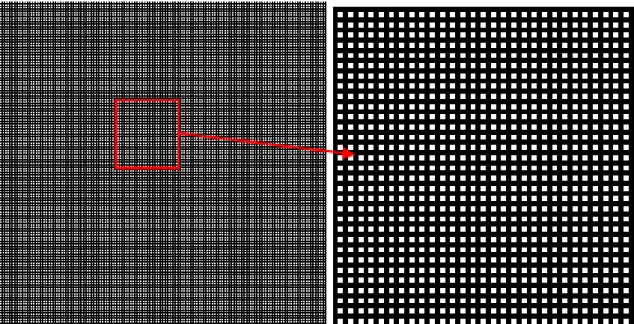
It is possible, however, to go further and to obtain a better labelling where the label values are consecutive1_{, from 1 to the total number of cells in the partition. To achieve this, the first step} consists in extracting the points of the image for which the previous label image is equal to the template image. For each cell of the partition, there exists one and only one pixel fulfilling this condition. Therefore, one could think that labelling this set of points would assign to each one a unique label value. Unfortunately, it is not the case because points belonging to different cells can nevertheless be connected and share the same label value. To cope with this problem, a further step is needed. For this, another template image must be generated. It is formed of a grid of points, each one been at a distance equal to 2 from its neighbors (Figure 9).

Figure 9: Grid of points used to separate adjacent points before labelling them. The right image is a zoom of the left one.

This set can be obtained very rapidly by simply extracting the lowest bit planes of the previous intermediary d1 and d2 distance images (remind that w and h are always even number in Mamba) and by intersecting them. By intersecting the initial set of points with this grid and with its three translations in the east, south and south-east directions, we split this set of 1

In fact, the label operator in Mamba does not produce a labelling with consecutive values. Some of them are not used. See the annex for further details.

(13)

points in four subsets of disconnected points which can be labelled. The four label images can then be combined to produce the final label image where each point is assigned a unique value. This combination is performed by adding to the current label image a constant value equal to the number of points already processed and by adding this current label image to the final one. This final label image is used through the cellsBuild procedure to get the final partion labelling. This procedure, called partitionLabel, is defined in the annex. This procedure returns the number of labelled cells. The procedure _generateTemplates, defining the two template images can also be found in the annex.

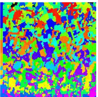
An example of such a dense labelling is shown in Figure 10. Remind, however, that some label values are not used (approximately 1 over 256). Note also that, contrary to the label procedure where missing values are multiple of 256, the missing values are distributed at irregular intervals.

Figure 10: Partition image (tools) labelling. The number of cells is equal to 1511, but the maximum label value is 65536, which means that many values have not been used.

3.2. Example of use

This partition labelling can be used to label partition cells with stereological measures. The procedure described for labelling binary partitions with measures (measureLabelling) can be used again. We just need to replace the initial label operator by this new partitionLabel operator. The partitionMeasureLabelling operator which can be found in the annex implements this procedure. Note that, due to the specific characteristic of the partition labelling (lack of some values), the parameter which controls the process is no longer the number of particles, but the maximum label value instead.

This operator can be used to label each cell of a partition with its area (Figure 11). We just have to use a filled image as the measure image in the operator. Each cell will be labelled with a value equal to the number of points it contains.

(14)

Other measures (diameters, connectivity numbers) can also be used. Getting the measure images can be performed by using the partition Hit-or-Miss transform, as it is defined in the MAMBA partition module (cellsHMT).

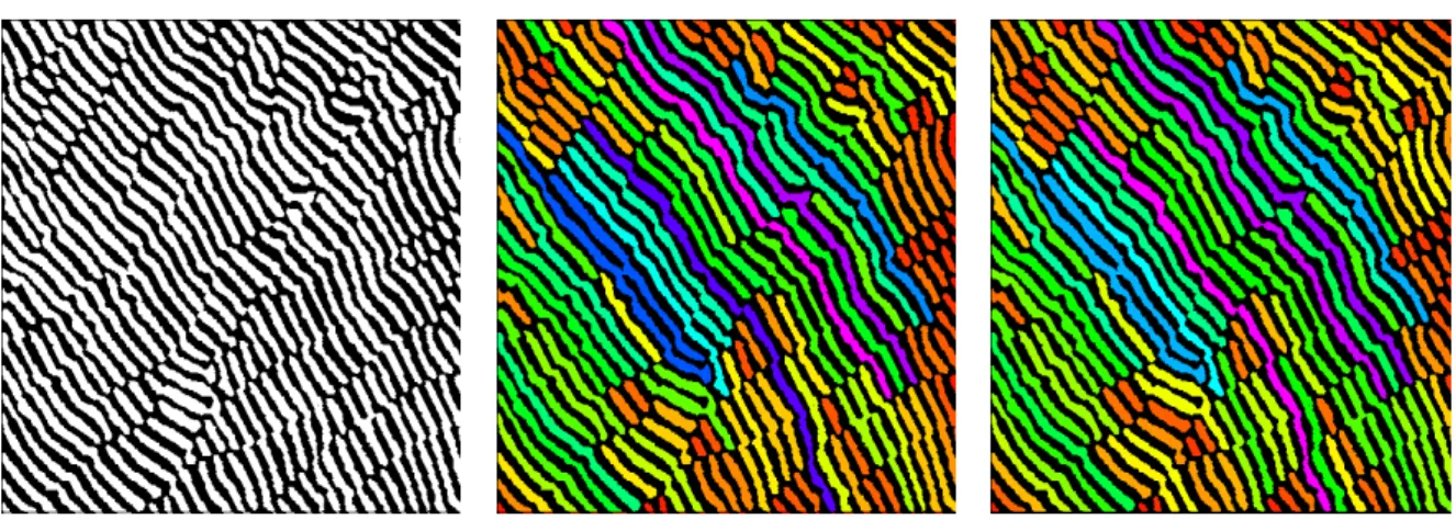
Figure 11: Area labelling of the tools partition image. 3.3. Other labellings

Labelling partitions with the Feret diameters of each cell is even simpler. The maximal coordinate labelling of each cell is produced by the cellsBuild operator with the marker image described in Figure 4. The minimal coordinate labelling is obtained with the dual cell reconstruction (I let the reader guess how to get it). The Feret diameter labelling of each cell is equal to the difference between these two intermediate label images.

4. Conclusions

As mentioned in the introduction, this paper does not describe any new concept. Its purpose is only to introduce various techniques to label sets or partitions.

Very often, measuring is the last step of an image analysis process. However, many powerful morphological operators, called adaptive transforms, are controlled by another image which indicates, for each pixel, either the kind of transformation to be applied locally or simply its size. This controlling image can be obtained by various means. It can be the result of another transform (as a residual transform for instance) or it can be produced by a local measure which is mapped on the image, hence the interest for the set labelling operators presented here.

Beside the examples described here, the reader will find other examples of this labelling in the MAMBA examples (traffic lanes segmentation, traffic measurement, vehicles detection and counting, segmentation of a heap of rocks for evaluating its size distribution). By allowing to design local measure maps, these labelling techniques change dramatically the

(15)

role of these measures in image analysis. They are no longer the final step of a process but, on the contrary, the starting point for a better control of adaptive operators.

Extending these labelling techniques to partitions is also of primary importance as many morphological operators can be applied on partitions which are considered as dual representations of graphs. It is the case, for instance, of the watershed transform or the hierarchical segmentations. Using partitions instead of graphs appears to be simpler because it is not necessary to build the graph and to transform again the result into an image at the end of the operation. Moreover, when the number of cells is important, using graphs becomes less and less effective. But working with partitions requires , on the one hand, efficient operators to deal with them and, in the other hand, flexible labelling algorithms to build them. These first operators are described in [1], whereas this note is devoted to the description of these labelling algorithms (which widely use partition operators).

Some of these operators extensively use algorithmic tricks in order to enhance their performance. Although this performance is supposed to be lower than a C/C++ language implementation would provide, we gain in flexibility and versatility. So, we hope that this document will provide some ideas for designing new specific labellings.

5. References

[1] Serge BEUCHER: Basic Morphological Operators Applied On Partitions. Web

publi-cation, March 2013. Available at http://cmm.ensmp.fr/~beucher/publi/Partitions.pdf.

[2] Serge BEUCHER: Measures in Mamba. Web publication, January 2011. Available at http://cmm.ensmp.fr/~beucher/publi/Measures in Mamba.pdf.

[3] Jean SERRA:Image Analysis and Mathematical Morphology - Academic Press, 1982.

6. Annex

The MAMBA source code of the various operators described in this document are given here. They work only with the version 1.1.3 of the library (released in June 2014).

Warning! The label operator in MAMBA does not use label values multiple of 256 (see the MAMBA user manual). This feature explains how some operators have been programmed. Note also that the partitionLabel operator does not use all the label values. However, the missed values are not necessarily multiple of 256.

"""

This module contains various labelling procedures for sets and for partitions. """

# Importing mamba and mambaComposed. from mamba import *

from mambaComposed import *

(16)

def areaLabelling(imIn, imOut):

"""

Labelling of each particle of the binary image 'imIn' with the value of its area. The result is put is the 32-bit image 'imOut'.

"""

# Working images.

imWrk1 = imageMb(imIn, 32)

imWrk2 = imageMb(imIn)

# Output image is emptied. imOut.reset()

# Labelling the initial image and setting the number of particles. nbParticles = label(imIn, imWrk1)

# Defining 4 output LUTs embedded in a single list. outLuts = [[0 for i in range(256)] for i in range(4)]

# Start of the loop. while nbParticles > 0:

# particles with labels between 1 and 255 are extracted.

# Mask of the values between 0 and 255 converted into a # greyscale image.

threshold(imWrk1, imWrk2, 0, 255)

convert(imWrk2, imWrk3)

# Extraction of the least significant byte plane of the label

# image and selection of the labels between 0 ans 255. copyBytePlane(imWrk1, 0, imWrk4)

logic(imWrk3, imWrk4, imWrk3, "inf")

# The histogram is computed. This operation is not performed

# on the image but simply on the histogram. histo = getHistogram(imWrk3)

# The same operation is performed for the 255 particles.

for i in range(1, 256):

# The area of each particle is obtained from the histogram.

value = histo[i]

j = 3

# The area value is splitted in powers of 256 and stored in the four

# output LUTs. while j >= 0: n = 2 ** (8 * j) outLuts[j][i] = value / n value = value % n j -= 1

# each LUT is used to label each byte plane of a temporary image with the

# corresponding value. for i in range(4):

lookup(imWrk3, imWrk5, outLuts[i])

copyBytePlane(imWrk5, i, imWrk6)

# The intermediary result is accumulated in the final image.

(17)

# 256 is subtracted from the initial labelled image in order to process

# the next 255 particles. substracting 256 (instead of 255) comes from the fact # that the label operator does not use label values which are multiple of # 256.

floorSubConst(imWrk1, 256, imWrk1)

nbParticles -= 255

# Note that the above area labelling can also be obtained by the following operation: # measureLabelling(imIn, imin, imOut)

# (See below).

# The measure labelling procedure is defined.

def measureLabelling(imIn, imMeasure, imOut):

"""

Labelling each particle of the binary image 'imIn' with the number of pixels in image 'imMeasure' contained in each particle. The result is put is the 32-bit image 'imOut'.

"""

# Working images.

imWrk2 = imageMb(imIn)

# Labelling the initial image. nbParticles = label(imIn, imWrk1)

# Defining output LUTs.

outLuts = [[0 for i in range(256)] for i in range(4)]

# Converting the imMeasure image to 8-bit. convert(imMeasure, imWrk4)

while nbParticles > 0:

copyBytePlane(imWrk1, 0, imWrk5)

# The points contained in each particle are labelled.

# The histogram is computed.

histo = getHistogram(imWrk5)

# The number of points in each particle is obtained from the histogram.

value = histo[i]

j = 3

# This value is splitted in powers of 256 and stored in the four

# output LUTs. while j >= 0:

(18)

n = 2 ** (8 * j)

outLuts[j][i] = value / n value = value % n j -= 1

logic(imOut, imWrk6, imOut, "sup")

# the next 255 particles (see above). floorSubConst(imWrk1, 256, imWrk1)

nbParticles -= 255

# The diameter labelling procedure is defined.

def diameterLabelling(imIn, imOut, dir, grid=DEFAULT_GRID):

"""

Labels each connected component of the binary image 'imIn' with its diameter in direction 'dir'. The labelled image is stored in the 32-bit image 'imOut'.

This procedure works on hexagonal or square grid. 'dir' can be any strictly positive integer value. """

dir = ((dir - 1)%(gridNeighbors(grid)/2)) +1 imWrk = imageMb(imIn)

# The intercept points in direction 'dir' are stored in imWrk. copy(imIn, imWrk)

diffNeighbor(imIn, imWrk, dir, grid=grid)

# They are used for the labelling. measureLabelling(imIn, imWrk, imOut)

# Labelling each particle with its number of holes (up to 1).

def holesLabelling(imIn, imOut, grid=DEFAULT_GRID):

"""

Labels each particle in 'imIn' with a value equal to its number of holes +1. The result is put in 32-bit image 'imOut'.

"""

# Working images. imWrk1 = imageMb(imIn)

# Initializing the label image with 2. convertByMask(imIn, imOut, 0, 2)

# The procedure on the hexagonal grid requires only two HMT operators. if grid == HEXAGONAL:

# Determining the 2nd configurations in the connectivity number calculation.

# and adding their number to the label image. hitOrMiss(imIn, imWrk1, 2, 5, grid=grid)

measureLabelling(imIn, imWrk1, imWrk2)

(19)

# Determining the 1st configurations and subtracting them to get the # number of holes + 1.

hitOrMiss(imIn, imWrk1, 66, 1, grid=grid)

# Whereas three MHT operators are required for the square grid. else:

# Second configuration points are extracted and used for the labelling.

add(imOut, imWrk2, imOut)

# First configurations are extracted and used for the labelling.

sub(imOut, imWrk2, imOut)

# Third configurations are processed.

hitOrMiss(imIn, imWrk, 40, 17, grid=grid)

sub(imOut, imWrk2, imOut)

def feretDiameterLabelling(imIn, imOut, direc):

"""

The Feret diameter of each connected component of the binary image 'imIn' is computed and its value labels the corresponding component. The labelled image is stored in the 32-bit image 'imOut'.

If 'direc' is "vertical", the vertical Feret diameter is computed. If it is set to "horizontal", the corresponding diameter is used.

"""

imWrk1.fill(1)

if direc == "horizontal":

dir = 7

elif direc == "vertical":

dir = 1

else:

dir = -1

# The above statement generates an error ('direc' is not horizontal or

# vertical.

# An horizontal or vertical distance function is generated.

linearErode(imWrk1, imWrk1, dir, grid=SQUARE, edge=EMPTY)

computeDistance(imWrk1, imOut, grid=SQUARE, edge=FILLED)

addConst(imOut, 1, imOut)

# Each particle is valued with the distance.

convertByMask(imIn, imWrk2, 0, computeMaxRange(imWrk3)[1])

logic(imOut, imWrk2, imWrk3, "inf")

# The valued image is preserved. copy(imWrk3, imWrk4)

# Each component is labelled by the maximal coordinate. build(imWrk2, imWrk3)

(20)

# Using the dual reconstruction, we label the particles with the # minimal ccordinate.

negate(imWrk2, imWrk2)

logic(imWrk2, imWrk4, imWrk4, "sup")

dualBuild(imWrk2, imWrk4)

# We subtract 1 because the selected coordinate must be outside the particle. subConst(imWrk4, 1, imWrk4)

negate(imWrk2, imWrk2)

# Then, the subtraction gives the Feret diameter. sub(imWrk3, imWrk4, imOut)

def volumeLabelling(imIn1, imIn2, imOut):

"""

Each connected component of the binary image 'imIn1' is labelled with the volume of the greyscale image 'imIn2' inside the this component. The result is put in the 32-bit image 'imOut'.

"""

imWrk1 = imageMb(imIn1)

imWrk2 = imageMb(imIn1, 32)

imWrk3 = imageMb(imIn1, 8)

imOut.reset()

n = imIn2.getDepth()

# Case of a 8-bit image. if n == 8:

for i in range(8):

# Each bit plane is extracted and used in the labelling.

copyBitPlane(imIn2, i, imWrk1)

measureLabelling(imIn1, imWrk1, imWrk2)

# The resulting labels are combined to obtain the final one.

v = 2 ** i

mulConst(imWrk2, v, imWrk2)

else:

for j in range(4):

# each byte plane is treated.

copyBytePlane(imIn2, j, imWrk3)

copyBitPlane(imWrk3, i, imWrk1)

measureLabelling(imIn1, imWrk1, imWrk2)

v = 2 ** (8 * j + i)

mulConst(imWrk2, v, imWrk2)

def _generateTemplates(imOut1, imOut2):

# this procedure generates two template images. The first one, 'imOut1', is # a 32-bit image where each pixel value is different. The second one, 'imOut2', # is a binary image containing a grid of points at a distance 2 apart.

imWrk1 = imageMb(imOut1, 1)

(21)

imWrk3 = imageMb(imOut1)

imWrk4 = imageMb(imOut1, 8)

imWrk1.fill(1)

# Generation of the first distance function.

linearErode(imWrk1, imWrk2, 7, grid=SQUARE, edge=EMPTY)

computeDistance(imWrk2, imWrk3, grid=SQUARE, edge=FILLED)

addConst(imWrk3, 1, imWrk3)

# Generation of the second distance function.

linearErode(imWrk1, imWrk2, 1, grid=SQUARE, edge=EMPTY)

computeDistance(imWrk2, imOut1, grid=SQUARE, edge=FILLED)

# Generation of the grid.

copyBitPlane(imWrk4, 0, imWrk2)

copyBytePlane(imOut1, 0, imWrk4)

copyBitPlane(imWrk4, 0, imOut2)

diff(imWrk2, imOut2, imOut2)

# Generation of the template image. w = imOut1.getSize()[0]

mulConst(imOut1, w, imOut1)

add(imOut1, imWrk3, imOut1)

def partitionLabel(imIn, imOut):

"""

This procedure labels each cell of image 'imIn' and puts the result in 'imOut'. The number of cells is returned. 'imIn' can be a 8-bit or a 32-bit image. 'imOut' is a 32-bit image.

Warning! The label values of adjacent cells are not necessarily consecutive.

"""

# generation of the two templates. _generateTemplates(imWrk1, imWrk2)

copy(imWrk1, imWrk3)

copy(imWrk2, imWrk6)

# The output image is reset. imOut.reset()

# if imIn is 8-bit, it is converted into a 32-bit image. if imIn.getDepth() == 8:

copyBytePlane(imIn, 0, imWrk4)

else:

copy(imIn, imWrk4)

# The initial imge is copied for later use. copy(imWrk4, imWrk7)

(22)

cellsBuild(imWrk4, imWrk3)

# Extraction of a single point in each cell.

generateSupMask(imWrk1, imWrk3, imWrk5, False)

nb = 0

v = 0

dir = 3

# Separation of the adjacent points and construction of the final # label image.

nb1 = label(imWrk6, imWrk4)

# Compute the maximal label value for the current points.

v1 = computeRange(imWrk4)[1]

convertByMask(imWrk6, imWrk3, 0, v)

add(imWrk4, imWrk3, imWrk3)

nb = nb + nb1 v = v + v1

shift(imWrk2, imWrk6, dir, 1, 0, grid=SQUARE)

dir += 1

cellsBuild(imWrk7, imOut)

return nb

def partitionMeasureLabelling(imIn, imMeasure, imOut):

"""

Labelling each cell of the greyscale or 32-bit image 'imIn' with the number of pixels in image 'imMeasure' contained in each particle. The result is put is the 32-bit image 'imOut'.

"""

# Working images.