HAL Id: hal-01686321
https://hal.archives-ouvertes.fr/hal-01686321
Submitted on 17 Jan 2018
HAL is a multi-disciplinary open access
archive for the deposit and dissemination of
sci-entific research documents, whether they are
pub-lished or not. The documents may come from
teaching and research institutions in France or
abroad, or from public or private research centers.
L’archive ouverte pluridisciplinaire HAL, est
destinée au dépôt et à la diffusion de documents
scientifiques de niveau recherche, publiés ou non,
émanant des établissements d’enseignement et de
recherche français ou étrangers, des laboratoires
publics ou privés.
Extending K-means to Preserve Spatial Connectivity
Sampriti Soor, Aditya Challa, Sravan Danda, B Daya Sagar, Laurent Najman
To cite this version:
Sampriti Soor, Aditya Challa, Sravan Danda, B Daya Sagar, Laurent Najman. Extending K-means
to Preserve Spatial Connectivity. IEEE International Geoscience and Remote Sensing Symposium
(IGARSS), Jul 2018, Valencia, Spain. �hal-01686321�
EXTENDING K-MEANS TO PRESERVE SPATIAL CONNECTIVITY
Sampriti Soor, Aditya Challa, Sravan Danda, B. S. Daya Sagar
Systems Science and Informatics Unit,
Indian Statistical Institute,
Bangalore, India.
Laurent Najman
ESIEE,
University Paris-Est,
Paris, France.
ABSTRACTClustering is one of the most important steps in the data pro-cessing pipeline. Of all the clustering techniques, perhaps the most widely used technique is K-Means. However, K-Means does not necessarily result in clusters which are spatially con-nected and hence the technique remains unusable for several remote sensing, geoscience and geographic information sci-ence (GISci) data. In this article, we propose an extension of K-Means algorithm which results in spatially connected clus-ters. We empirically verify that this indeed is true and use the proposed algorithm to obtain most significant group of wa-terbodies mapped from multispectral image acquired by IRS LISS-III satellite.
Index Terms— Clustering, Graphs, K-Means 1. INTRODUCTION
Clustering is one of the most important steps in data min-ing and machine learnmin-ing [1, 2, 3]. Clustermin-ing has been used across several data domains ranging from text processing to hyperspectral images. Clustering in the context of image data is also referred to as segmentation. Thanks to its unsupervised nature, it can be used for several tasks such as simplifying and understanding the data, visualizing the important aspects etc. Due to the same reason, the solution to the problem of cluster-ing is also extremely dependent on the domain of application. This requires adapting the existing methods to the domain, ensuring that the appropriate properties are preserved. In this article, we tackle one such problem - using K-Means while preserving spatial connectivity.
K-Means is one of the most widely used methods for clus-tering data [1, 4]. It is categorized under partition based methodsand has some very important properties. It has been shown that using expectation maximization idea for cluster-ing gaussian mixture models is closely related to the K-means method [3]. It is also very efficient and variations of k-means are also used for clustering big-data. K-means used along with map-reduce framework was proposed in [5]. However, for segmentation it is seen that k-means does not preserve the spatial connectivity of the final clusters. This property of connectedness of the clusters is important in the context
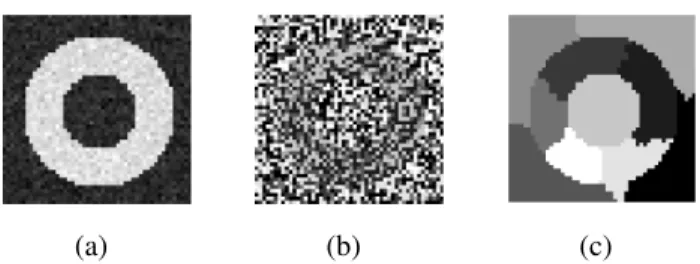
(a) (b) (c)
Fig. 1. An example showing that K-means does not ensure the connectivity of the clusters. (a) Original Image - Simple image with gaussian noise. (b) Clustering result obtained by using simple K- Means without any constraint on connectiv-ity. Number of clusters is taken to be 10. (c) Clustering result obtained using the proposed algorithm 1, which performs K-Means with constraint on connectivity. Number of clusters is taken to be 10
of remotely sensed spatial images and hence K-Means cannot be directly used. For instance consider the image in figure 1(a). When simple K-Means is used in this case, we obtain the result as in figure 1(b), with number of clusters fixed at 10. Note that the final clustering is highly noisy. The reason for this is because, classical K-Means algorithm does not take into consideration the connectivity of the data.
In this article, we propose an algorithm which extends the classical K-Means algorithm to preserve the connectivity of the final clusters. The result of this algorithm on figure 1(a) is shown in figure 1(c). This is the main contribution of this article. The description of the algorithm is given in section 3, and the fact that the proposed algorithm is indeed an extension of K-Means is verified empirically on toy datasets. We then show an application of the proposed algorithm to obtain k most significant waterbodies mapped from multispectral im-age taken from IRS LISS-III satellite in section 4.
2. REVIEW
K-Means is a simple algorithm which is widely used in literature [6]. The algorithm starts with picking K initial points as the centroid and repeating the following steps until
convergence-1. Form K clusters by assigning every point to the closest of the K initial points.
2. Recalculate the centers of the K clusters.
Assume that we have a clustering C = {C1, C2, · · · , CK},
then, squared sum of errors (SSE) is defined by
SSE(C) = K X k=1 X xi∈Ci d(xi, ci) (1)
where xidenotes the points, cidenotes the center of the
clus-ter Ciand d(., .) denotes the distance metric. It can be shown
that K-Means algorithm works by monotonically reducing the SSE error function until it reaches a local minima. (See chapter 4 of [3] for details.)
In this article, we aim to extend the K-Means technique with an additional constraint of resulting in clusters which are connected. This requires specifying the adjacency relation in the problem statement, thus allowing to maintain the connec-tivity of the clusters. We achieve this by using the framework of the edge-weighted graphs.
An edge weighted graph G = (V, E, W ) is a tuple with three sets - a set of nodes/vertices where each node/vertex denotes each data point, a set of edges which defines the adja-cency relation on the given data and a function W : E → R+
which denotes the weight of each edge.
Also, one of the important steps of the K-Means algorithm is to calculate the ‘mean’ of the objects in the cluster. This however, is not always possible in general since objects need not necessarily belong to a space where averages are defined. This is especially common in the field of geoscience and re-mote sensing. For instance, consider the problem of clus-tering of water bodies (discussed in [7]), or more abstractly sets in the euclidean space. Thus in this article we consider a variant of the K-Means algorithm, known as K-Medoids (see chapter 4 of [3] for more details) where the center is taken to be one of the data points in the set.
3. EXTENDING K-MEANS TO EDGE WEIGHTED GRAPHS
Thus, the problem of clustering becomes minimizing the op-timization problem in (1) subject to the constraint that each cluster Ciis connected with respect to the adjacency relation
given by E. To solve this minimization problem, we propose the algorithm 1.
The algorithm proceeds similarly to the K-Means algo-rithm and starts with picking out K random seeds from the data. At each stage, all the nodes are assigned to the nearest reachable seed, that is there exists a path between the node and a seed and all the nodes in the path are assigned to this seed. This is achieved by using a priority queue, where the
Algorithm 1 K-means with connectivity constraint Input: An edge weighted graph, G = (V, E, W ) Output: C = {C1, C2, · · · , CK} - K clusters
1: Pick K random points from the set of nodes V as initial seeds.
2: while Convergence is not reached do
3: Initialize a priority queue - Q and a set data structure P . P indicates the set of pixels already processed.
4: Push all the neighbors of the seeds into Q, where pri-ority is given by the distance to the node
5: while Q is not empty do
6: Pop the vertex v from Q
7: if v is not in P then
8: Assign it to the nearest seed and add it to the set P .
9: for each neighbor u of v do
10: Push the neighbor w into Q, with priority given by
priority(u) = W (v, u) + priority(v)
11: end for
12: end if
13: end while
14: Update the centers of each cluster with the node that minimizes the largest distance.
15: end while
priority is given by the distance to the node. These priorities are updated lazily to ensure efficient implementation. This en-sures the connectedness of the component once all the nodes are processed as described by the proposition 1.
Proposition 1. For every iteration between steps 3-12 in al-gorithm 1, the connectedness of the cluster is preserved.
The seeds are then recalculated. For each component, the new seed is taken to be the center of the subgraph. Given the distance d(., .), the center of the graph is defined as
arg min x X u d(x, u) (2)
Empirical Verification
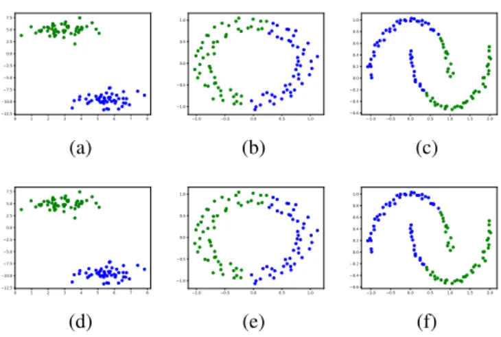
To illustrate the fact that the algorithm 1 is an extension of K-Means to graphs, we perform the following experiment. Ob-serve that, any theoretical extension of K-Means to graphs should match with K-Means on the complete graph1. Since, on a complete graph any two nodes are adjacent, the con-straint on connectivity is nullified. Another way to interpret this by considering a neighborhood matrix, whose entries are 0/1, which gives the neighborhood relation between the two
0 1 2 3 4 5 6 7 8 −12.5 −10.0 −7.5 −5.0 −2.5 0.0 2.5 5.0 7.5 (a) −1.0 −0.5 0.0 0.5 1.0 −1.0 −0.5 0.0 0.5 1.0 (b) −1.0 −0.5 0.0 0.5 1.0 1.5 2.0 −0.6 −0.4 −0.2 0.0 0.2 0.4 0.6 0.8 1.0 (c) 0 1 2 3 4 5 6 7 8 −12.5 −10.0 −7.5 −5.0 −2.5 0.0 2.5 5.0 7.5 (d) −1.0 −0.5 0.0 0.5 1.0 −1.0 −0.5 0.0 0.5 1.0 (e) −1.0 −0.5 0.0 0.5 1.0 1.5 2.0 −0.6 −0.4 −0.2 0.0 0.2 0.4 0.6 0.8 1.0 (f)
Fig. 2. Illustration showing that the results of the proposed algorithm 1 on a complete graph indeed match the ones of K-means. Top row: Result of clustering obtained on toy ex-amples using K-Medoids. Bottom row: Result of clustering obtained on toy examples using algorithm 1 with complete graph.
pixels. In the degenerate case of all entries in the neighbor-hood matrix being 1, the algorithm 1 reduces to K-Means. Figure 2 shows a typical results obtained using the K-Medoids and algorithm 1.
Remark: The proposed algorithm can be seen as an it-erated version of the classical watershed algorithm used in image segmentation [8], where the seeds of the watershed are updated after each watershed step.
4. APPLICATION
As an application of the proposed algorithm we consider wa-ter bodies data taken from [7]. In [7], this data was used to identify the waterbody which is spatially significant. How-ever, the problem can be extended to identify the most sig-nificant k water bodies. This type of analysis can be used for policy planning. Observe that identifying the top k significant waterbodies can be phrased in the framework of K-Means, where one can cluster the waterbodies and identify the cen-ters (spatially significant points). This is an example where algorithm 1 is useful.
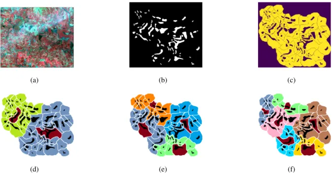
In figure 3(a) we have the multispectral data from which the water bodies are mapped as in figure 3(b). The question of interest is to identify the most significant k waterbodies from the data. The significant waterbody is defined as the waterbody which is placed closest to all other waterbodies in the cluster. For this we use the dilation distance [7] as the distance between the waterbodies. Given two sets S1and S2,
the dilation distance is defined as
d(S1, S2) = inf{λ | S1⊕ λB ⊇ S2} (3)
where B is a unit disk structuring element. The adjacency relation is obtained by the influence zones of figure 3(b), as shown in figure 3(c). Two waterbodies are considered adja-cent, if their influence zones are adjacent in figure 3(c). Using these parameters, significant waterbodies for k = 2, 4, 6 are calculated as shown in figure 3 (d)-(f).
5. CONCLUSION AND FUTURE WORK
In summary, we have proposed an algorithm which extends the K-Means to obtain clusters which are connected. This is achieved by considering the framework of edge graphs. The algorithm obtained was shown to give consistent results with a variant of K-Means in the degenerate case of considering a complete graph. This was then applied to the waterbodies data from [7] to obtain k = 2, 4, 6 significant waterbodies.
In future, on the theoretical front, we hope to obtain a rig-orous proof of equivalence between algorithm 1 and K-Means technique. On the application front we expect to use the al-gorithm proposed to various other data and perform extensive validation.
6. ACKNOWLEDGMENTS
The first three authors would like to thank Indian Statisti-cal Institute for the funding provided. BSDS would like to acknowledge the support received from the Science and Engineering Research Board (SERB) of the Department of Science and Technology (DST) with the grant number EMR/2015/000853, and the Indian Space Research Organi-zation (ISRO) with the grant number ISRO/SSPO/Ch-1/2016-17.
7. APPENDIX : PROOF OF PROPOSITION 1
Proof. We only provide the idea of the proof here. Let S = {si} indicate the seeds and d(u, w) indicate the distance
be-tween u and w. We assume that the distance metric used sat-isfies the regularity conditions mentioned in [9]. From the algorithm it is clear that a node u is assigned to the seed si
which minimizes d(u, si).
We show that if u is assigned to the seed si, then the nodes
in the shortest path < u, si> are also assigned to si. Assume
for the sake of contradiction that v is assigned to sj, j 6= i.
This implies that d(v, sj) < d(v, si). Thus,
d(u, si) = d(u, v) + d(v, si)
> d(u, v) + d(v, sJ)
> d(u, sj)
Hence we get a contradiction. So, all the nodes in the shortest path belong to the component, and hence it is connected.
(a) (b) (c)
(d) (e) (f)
Fig. 3. Application of algorithm 1 to waterbodies clustering. Top row : (a) Multispectral image acquired by IRS LISS-III satellite. Blue objects indicate the waterbodies. (b) Waterbodies mapped from the image in (a). (c) Influence zones of the waterbodies in (b). Bottom row: Clustering obtained using algorithm 1. The red color influence zone indicates seed of the cluster, which is also the most significant waterbody in that cluster. The number of clusters taken are - (d) k = 2 (e) k = 4 (f) k = 6
8. REFERENCES
[1] Anil K Jain, “Data clustering: 50 years beyond k-means,” Pattern Recognition Letters, vol. 31, no. 8, pp. 651–666, 2010.
[2] Anil K Jain, M Narasimha Murty, and Patrick J Flynn, “Data clustering: a review,” ACM Computing Surveys (CSUR), vol. 31, no. 3, pp. 264–323, 1999.
[3] Charu C. Aggarwal and Chandan K. Reddy, Data Clustering: Algorithms and Applications, Chapman & Hall/CRC, 1st edition, 2013.
[4] David Arthur and Sergei Vassilvitskii, “k-means++: The advantages of careful seeding,” in Proceedings of the eighteenth annual ACM-SIAM Symposium on Discrete Algorithms. Society for Industrial and Applied Mathe-matics, 2007, pp. 1027–1035.
[5] Weizhong Zhao, Huifang Ma, and Qing He, “Parallel k-means clustering based on mapreduce,” in IEEE Interna-tional Conference on Cloud Computing. Springer, 2009, pp. 674–679.
[6] James MacQueen et al., “Some methods for classifica-tion and analysis of multivariate observaclassifica-tions,” in Pro-ceedings of the fifth Berkeley Symposium on
mathemati-cal statistics and probability. Oakland, CA, USA., 1967, vol. 1, pp. 281–297.
[7] B. S. D. Sagar, N. Rajesh, S. Ashok Vardhan, and P. Vard-han, “Metric based on morphological dilation for the de-tection of spatially significant zones,” IEEE Geoscience and Remote Sensing Letters, vol. 10, no. 3, pp. 500–504, 2013.
[8] Jean Cousty, Gilles Bertrand, Laurent Najman, and Michel Couprie, “Watershed cuts: Minimum spanning forests and the drop of water principle,” IEEE Transac-tions on Pattern Analysis and Machine Intelligence, vol. 31, no. 8, pp. 1362–1374, 2009.
[9] Alexandre X Falc˜ao, Jorge Stolfi, and Roberto de Alen-car Lotufo, “The image foresting transform: Theory, al-gorithms, and applications,” IEEE Transactions on Pat-tern Analysis and Machine Intelligence, vol. 26, no. 1, pp. 19–29, 2004.