Choosing Internet Paths with High Bulk Transfer Capacity
by
Jacob A. Strauss
S.B., Massachusetts Institute of Technology (2001)
Submitted to the Department of Electrical Engineering and Computer Science
in partial fulfillment of the requirements for the degree of
Master of Engineering in Electrical Engineering and Computer Science
at the
MASSACHUSETTS INSTITUTE OF TECHNOLOGY
September 2002
0
Jacob A. Strauss, MMII. All rights reserved.
The author hereby grants to MIT permission to reproduce and distribute publicly
paper and electronic copies of this thesis and to grant others the right to do so.
A u th o r ...
. . ..
.. ... ...Department gElectrical Engineering and Computer Science
September 3, 2002
C ertified by ... -... . ...
M. Fi ns Kaashoek
ProfessornrTfomputer Science and Engineering
Thesis Supervisor
C ertified by ...
...
Robert T. Morris
Assistant Professor of Computer Science and Engineering
Thesis Supervisor
Accepted by ...
Arthur C. Smith
Chairman, Department Committee on Graduate Students
MASSACHUSETTS INSTITUTE OF TECHNOLOGY
Choosing Internet Paths with High Bulk Transfer Capacity
by
Jacob A. Strauss
Submitted to the Department of Electrical Engineering and Computer Science on September 3, 2002, in partial fulfillment of the
requirements for the degree of
Master of Engineering in Electrical Engineering and Computer Science
Abstract
Many applications wish to predict what bandwidth TCP can achieve on a path between Internet hosts without performing extensive measurements. More precisely, they would like to know the bulk transfer capacity (BTC) of a given path. This thesis compares the ability of several BTC estimation methods to predict which of a pair of Internet paths will have the higher measured BTC. Methods tested include TCP loss rate models, an available bandwidth measuring tool named Pathload [17], path capacity measurements, Asymptotic Dispersion Rate measurements, and a new approach we call Squeezed Pairs. We tested each estimation method on paths between hosts on the RON testbed [5]. When taking measurement costs into account, the best method we have found to pick the faster of a pair of paths determines the Asymptotic Dispersion Rate of each path. The ADR test consists of sending two streams of 15 packets back-to-back and calculating the average spacing between probe packets at the receiver. The ADR test correctly predicts which path will have a higher BTC in 80% of all path pairings.
Thesis Supervisor: M. Frans Kaashoek
Title: Professor of Computer Science and Engineering Thesis Supervisor: Robert T. Morris
Acknowledgments
This work was supported by the Defense Advanced Research Projects Agency (DARPA) and the Space and Naval Warfare Systems Center, San Diego, under contract N66001-00-1-8933.
I wish to thank:
Frans, for his ever useful advice and encouragement.
Robert, Dina, Hari, & Chuck, for their insights, experience, and guidance. Dave, for making the whole project possible.
My parents, for all that they have done.
Contents
1
Introduction 81.1 Resilient Overlay Networks . . . . 8
1.2 D efinitions . . . . 9
1.3 Bulk Transfer Capacity Properties . . . . 11
1.4 Contributions . . . . 12
1.5 O verview . . . . 12
2 Related Work 13 2.1 Capacity Estimation . . . . 13
2.2 Bulk Transfer Capacity Estimation . . . . 14
2.2.1 TCP and TCP emulators . . . . 14
2.2.2 TCP models . . . . 14
2.3 Available Bandwidth Estimation . . . . 15
2.4 Property Constancy . . . . 16
3 BTC Estimation Methods 17 3.1 T C P . . . . 17
3.2 Loss Rate ... ... ... ... 18
3.3 Asymptotic Dispersion Rate . . . . 18
3.4 P athload . . . . 19
3.5 Squeezed Pairs . . . . 19
4 Methodology 26 4.1 B T C Tests . . . . 26
4.1.2 Asymptotic Dispersion Rate . . . . . 4.1.3 Squeezed Pair test . . . . 4.1.4 Pathload . . . .
4.1.5 TCP test . . . .
4.1.6 Capacity Measurements . . . . 4.1.7 Loaded Paths . . . . 4.2 Processing . . . . 4.3 From Test Phases to BTC Estimates . . . .
5 Path Choosing Results
5.1 Method Comparisons . . . .
5.1.1 Measurement Costs . . . . 5.1.2 All path pairs . . . . 5.1.3 Common Endpoint Pairs . . . . 5.2 Using Squeezed Pairs to pick an appropriate
5.3 Correlations Between Methods . . . . 5.4 Investigating Failures . . . . 5.4.1 Short TCP Transfers . . . . 5.4.2 RON Loss probes . . . .
5.4.3 Pathload . . . .
5.5 Path Choosing on Loaded paths . . . . 5.6 Sum m ary . . . .
6 Predicting TCP Performance 6.1 TCP predicting TCP . . . . . 6.2 Pathload . . . .
6.3 RON loss scoring . . . .
6.4 ADR . . . .
6.5 Path Capacity . . . . 6.6 Pathload with Squeezed Pairs
6.7 Summary . . . .
7 Conclusion and Future Work
method 27 27 28 28 29 29 29 30 32 33 33 34 35 36 38 40 40 40 40 41 41 43 43 45 46 48 48 49 51 52
List of Figures
3-1 Squeezed Pairs on an idle path . . . .
3-2 Squeezed Pairs on a tight-like-narrow path .
3-3 Squeezed Pairs on a tight-unlike-narrow path
TCP prefixes vs TCP . . . .
Pathload vs TCP . . . . RON loss scoring vs TCP . . . . RON lossonly paths vs TCP . . . .
ADR vs TCP . . . .
Path Capacity vs TCP . . . .
Pathload vs TCP by Squeezed Pairs classification .
. . . . 44 . . . . 45 . . . . 46 . . . . 47 . . . . 48 . . . . 49 . . . . 50 21 22 23 6-1 6-2 6-3 6-4 6-5 6-6 6-7
List of Tables
4.1 RON sites and locations . . . . 27
5.1 All-Pairs decision rates . . . . 32
5.2 BTC Estimation costs . . . . 34
5.3 Common Endpoint Decision Rates . . . . 35
5.4 Tight-like-narrow decision rates . . . . 36
5.5 Tight-unlike-narrow decision rates . . . . 37
5.6 Combined tight-like-narrow and tight-unlike-narrow decision rates . . . . . 37
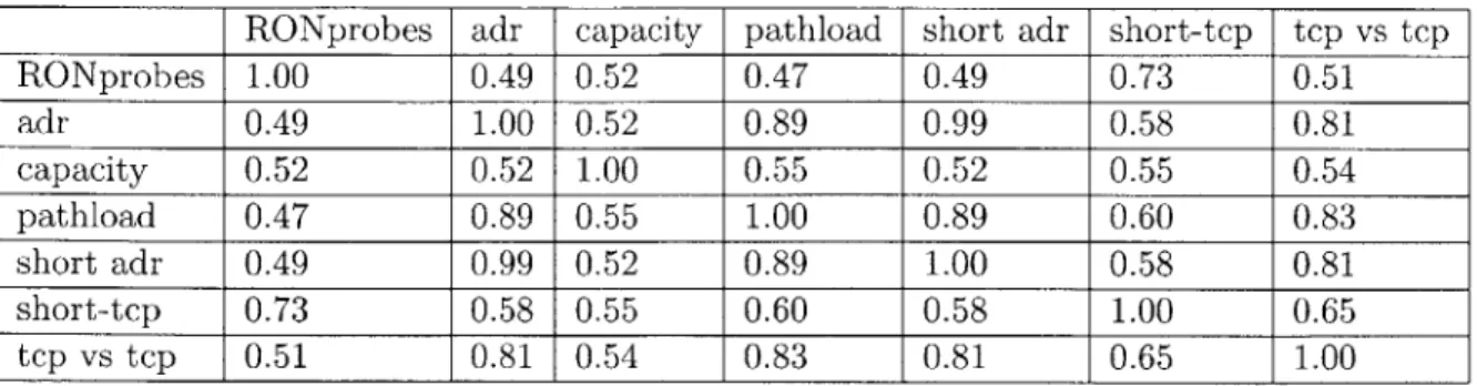
5.7 Correlations between Decision Methods . . . . 39
Chapter 1
Introduction
Predictions of end-to-end bulk transfer capacity, or BTC for short, between Internet hosts are useful for overlay networks, congestion control, streaming media, and network monitor-ing applications. For example, resilient overlay networks (RONs) can use BTC knowledge to select the Internet path that will achieve the highest TCP throughput [5]. In this thesis, we compare various methods for picking the path with higher BTC among pairs of paths between machines in the RON testbed.
Existing methods used to measure BTC are intrusive, sending large amounts of probe traffic, which interferes with other flows using the same path. Effective non-intrusive mea-surement methods do exist for other end-to-end path characteristics such as path capacity and available bandwidth, but not for BTC.
In addition to comparing BTC estimates on different paths, we compare BTC estimates with BTC measurements to gauge estimation error. These comparisons are useful for ap-plications that wish to know whether a given path can support a specific transfer rate.
We test BTC estimation methods on the RON testbed, a set of measurement machines spread throughout the Internet. The RON testbed was constructed to evaluate the per-formance of resilient overlay networks. We do not use any of RON's intermediate host forwarding mechanisms in our experiments.
1.1
Resilient Overlay Networks
RON [5, 6] is an overlay network that uses a collection of cooperating hosts spread through the Internet to provide communication between hosts that is better in metrics such as loss
rate, latency, and throughput than the underlying Internet alone provides.
RON takes advantage of underlying multiplicity in routes between Internet hosts to pick good paths over poor ones. The direct Internet path between a given pair of hosts is determined only by the routers along the path. RON can choose an indirect path whereby packets are first sent to another RON host and forwarded from there to the actual destina-tion. RON can therefore choose between the direct Internet path, and a number of paths that include one or more intermediate RON nodes.
Applications using RON can specify a preference for a latency-optimized path, a loss-optimized path, or a bandwidth-loss-optimized path. This work examines RON's method for choosing paths when applications desire a bandwidth-optimized path.
In order to choose between paths, RON hosts send periodic pings to each other to measure loss rates and latency. These probes are effective at choosing routes which minimize low loss rate and end-to-end latency. The probes, however, are not sufficient to choose the path with highest BTC in most cases.
Any method used to probe BTC values between RON nodes must constrain the amount of measurement traffic required to produce useful estimates. RON gathers information about each path between participating hosts, and must ensure that the sum total of probe traffic to each of its peers does not consume a burdensome portion of resources available to that host. For example, in a RON network consisting of 50 nodes, each host must allow for 49 times the probe traffic to any single peer.
1.2
Definitions
We will use the terms: bulk transfer capacity, available bandwidth, path capacity, link capacity, narrow link, and tight link, throughout this thesis. Not all related work assigns the same meaning to these terms, especially available bandwidth and bulk transfer capacity. To avoid confusion, we define these terms here before continuing. The definitions here are the same as in much of the recent related work [11, 16, 17, 4, 24].
Consider the path between two hosts on the Internet, from A to B. This path is made up of n links, each of which has a link capacity, ci through cn. Each link capacity is the fastest rate at which packets can be forwarded over that link. The path capacity from A to B is mingi...n(ci). We call the link with smallest capacity ci the narrow link from A
to B. There may be more than one narrow link along a path, in which case the capacity of each must be the same. We assume that link capacities change rarely; they should only change with either a route change, or a physical change to the underlying links. In the RON testbed, narrow links are almost always no more than a few hops away from RON machines. As such, we assume that ci is constant for the duration of one test, which may last as long as a half hour.
Each link has a current utilization ui. Utilization is the proportion of that links' capacity which is used over some time interval. 1 - ui is the idle fraction of that link for the same interval. The unused capacity on each link is ci(1 - ui).
The available bandwidth from A to B is mini=1..., ci(1 - ui). The tight link is the link
from A to B with smallest unused capacity. As with narrow links, there may be more than one tight link in a single path if queuing due to competing traffic or dropped packets occurs at more than one link.
The bulk transfer capacity, as described by Mathis and Allman [241, is the fastest rate a protocol that implements TCP-friendly congestion control can forward packets from A to B. TCP is one example of such a protocol, which we use to measure BTC. BTC depends only on network conditions and the choice of which congestion control algorithm to use. For example, buffer space on routers between A and B, queuing policies, and cross traffic on all hops will affect BTC. Buffer space available on A or B does not, as we require that BTC transfers not be limited by resources in the end hosts. An example setup to measure BTC is Reno TCP with unlimited receiver window size, MTU set to the maximum size which avoids IP fragmentation, infinite-length transfer, and end hosts sufficiently fast that packet processing time is insignificant. Like available bandwidth, BTC is a time dependent quantity. Unless stated otherwise, we refer to averages over periods of several seconds to a minute for BTC and available bandwidth.
Consider a simple example to illustrate the difference between available bandwidth and BTC. A path consisting of a single 1 Mbps link clearly has a path capacity of 1 Mbps. Let this path be idle except for a single TCP flow transmitting at 1 Mbps. The available bandwidth of this path is 0 Mbps, since there is no unused capacity. The BTC of this path is 0.5 Mbps, as a second TCP connection started over the path would eventually claim half of the total capacity.
from A to B is in general different than the capacity or BTC from B to A.
1.3
Bulk Transfer Capacity Properties
In many applications, BTC is the metric that best describes the performance of an Internet path. Capacity and available bandwidth measurements are in essence one step removed from BTC values. Capacity describes the quiescent network state, while available bandwidth describes load on the routers along a given path. For any application that is considering using the path and wishes an estimate of what the network will support, or picking between paths, neither capacity estimates nor available bandwidth adequately describe end-to-end performance. However, we have effective non-intrusive methods to measure capacity and available bandwidth, and none for BTC.
Why is BTC hard to measure? Unlike capacity and available bandwidth, we lack a
simple way to express BTC in terms of network observables. BTC is instead described in terms of TCP's congestion control algorithms [15][3].
TCP throughput is affected by many different factors, which include latency and ca-pacity of every link, nature of competing traffic at each link, router queuing policy and buffer sizes, link-level performance, reverse path conditions, and data corruption, among other factors. The Amherst model [27], expresses TCP throughput in terms of observed loss rate along with measurable parameters such as round trip time, and TCP implementation. However, a flow's loss rate cannot be predicted from other information easily. Goyal et al. [13] tried to refine this model to use loss rates obtained from routers along the path in question. However, their estimates required a high correlation between TCP loss rates and earlier measurements of router drop rates.
Bulk transfer capacity would be much easier to measure in networks consisting of XCP routers [19]. Unlike TCP routers, it is easy to express the expected long term BTC in terms of available bandwidth at each XCP router and characteristics of cross traffic flows. Moreover, XCP does not use slow start, and congestion window sizes converge to an average value faster than in TCP flows, so throughput for short flows should not differ greatly from throughput in long flows.
1.4
Contributions
This thesis compares the accuracy and measurement costs of a number of possible methods to measure BTC, including one novel approach. We evaluate the methods both on their ability to compare different paths and estimate which has higher BTC, and their ability to produce a numerical BTC estimate. We show that all of the non-intrusive methods are often incorrect by several orders of magnitude in numerical BTC estimates, though several non-intrusive methods are useful for choosing between paths.
We recommends a replacement for RON's method of choosing bandwidth-optimized paths. We show that the current method provides far from ideal performance, and propose
a replacement that is simple and more effective, and only moderately expensive to deploy. Finally, much related work on capacity and load estimates uses simulation and measure-ments over a few Internet paths. Only a few such methods have been tested over a wide variety of Internet paths. This work offers some practical experience of using a number of tools under real network conditions.
1.5
Overview
The remainder of this thesis is structured as follows. Chapter 2 discusses related work. Chapter 3 describes the measurement methods that we chose to examine. Chapter 4 details the experiments conducted over RON. Results pertaining to path choosing are discussed in
Chapter 5. Comparisons between estimated BTC and measured BTC are in chapter 6. We conclude with recommendations based on the results and areas for future work.
Chapter 2
Related Work
Many of the methods used to measure path properties such as capacity and available band-width are applicable toward BTC estimation. We describe serveral of these measurement methods, and discuss limitations of existing approaches for BTC measurement.
2.1
Capacity Estimation
Packet pair is the base method that is used in the most efficient methods of measuring path capacity. Packet pair was described by Keshav [20]. Its simplicity and wide use warrants a detailed explanation.
Consider a pair of hosts separated by a path of capacity C. The source host sends a pair of packets back-to-back each with size L. Assuming that these packets are uninfluenced
by competing traffic on any of the links between the source and destination, the two probe
packets will arrive at the narrow link between source and destination close enough that they will traverse the narrow link between back-to-back. At the narrow link, the packets will be spaced in time by At = L/C. All links after the narrow link will preserve this spacing. The destination then measures the difference between the arrival times of the two packets, and computes C as L/At.
In paths with cross traffic, however, the spacing at the receiver can be both larger and smaller than the spacing set solely by the capacity of the narrow link. If the pair traverses the narrow link with a cross traffic packet in between, then the packet spacing at the destination will be larger than capacity alone would dictate. If the first packet is delayed at a router after the narrow link, causing the pair to queue together, then the spacing at
the destination will be smaller than L/C.
The spacing also depends on the queing policy employed by the router. Packet pair will compute capacity when the routers use first-come-first-served queuing, but will instead compute a value lower than the path capacity if the routers employ fair queuing algorithms. Multipath links, traffic shapers, and end host load further complicate measurements.
All of the successful projects that measure path capacity make use of the packet pair
approach, either entirely, or as a base method. Each tool supplements packet pair and filters valid results to a varying degree.
Nettimer [21], Packet Bunch Modes [29], bprobe [9], and Pathrate [11] all discuss meth-ods for filtering packet pair measurements to determine path capacity. Pathchar [14] deter-mines hop-by-hop capacity.
2.2
Bulk Transfer Capacity Estimation
There are two current methods for estimating BTC. The first is to emulate TCP, which requires long measurement times and also a large amount of probe data. The second method is to use a bandwidth model for TCP based on packet loss rates. This reliance on loss rates makes makes TCP models good at describing bandwidth retrospectively, but are not good predictors in the absence of a current flow.
2.2.1 TCP and TCP emulators
Tools to measure BTC include Treno [23] and cap [4]. Both tools aim to abstract away the details of TCP implementations, but they still require long and intrusive measurements in order to obtain accurate results. Allman found that BTC values reported by cap generally agreed with the BSD TCP implementation to within 10% [4]. We use TCP as implemented directly by FreeBSD directly in our measurements, and assume that rates we observed are close to the BTC. We ignore any possible effects variations between TCP implementations.
2.2.2 TCP models
The Amherst model [27] estimates the throughput of a steady-state TCP flow. The model treats a TCP connection as a sequence of rounds, which generally consist of a set of packets sent nearly back-to-back within one RTT. The model assumes that packet losses in separate
rounds are independent, while within each round all packets after the first drop are also dropped. This assumption may be reasonable for DropTail routers, but not RED routers. Rounds with no packet losses cause the sender to increase its congestion window, and losses make the sender shrink the congestion window size just as real TCP implementations do. The model then computes the expected round length, and expected window size over the course of the flow in terms of the RTT and loss rate. The following expression is an approximation of the model's result for TCP throughput, in packets per second:
(Wm 1
B(p) ~ min - max I -(2.1)
RTT' RTT $2 + T min 1, 3 p(+ 32p2)
The round trip time between sender and receiver is RTT, Wmax is the maximum receiver window size, b is the the number of packets acknowledged with each ACK, and To is the
initial sender retransmission timeout. The Amherst model assumes that packet losses are independent when packets are sent at well-spaced times, but that losses are highly correlated between packets sent back-to-back. Using this assumption, the model breaks up a transfer into a number of rounds. The packet loss probability p, is the probability that a packet is lost when it is either the first packet in a round or none of the earlier packets in that round were lost. TCP receivers that implement delayed acks commonly use 2 as the value for b.
This model was revised by Goyal et al. [13] to use the overall packet loss probability, rather than the conditional probability based on the position of a packet within a round. They used their new model to predict TCP throughput based on packet loss probabilites reported by the tight link router. This approach is not possible when statistics from the tight link are not available, and when there are no end-to-end observable losses.
These two approaches both require accurate knowledge of the frequency of loss events. In the case of traditional TCP, this is the same as lost packets, though for an ECN-enabled sender [12, 30] this would include both lost packets and packets marked as experiencing congestion.
2.3
Available Bandwidth Estimation
Pathload [17, 16], which we use in our measurements, uses Self Loading Periodic Streams to measure available bandwidth. Self Loading Streams measure available bandwidth by
sending short bursts of evenly spaced packets and observing increasing queueing delays over the course of the burst. Sending bursts at rates below the available bandwidth does not cause increasing trend through the course of the burst. By starting with an initial estimate of the Aymptotic Dispersion Rate [11, an iterative search proceeds between rates that show increasing trends and rates which do not. Each rate tested currently requires a large amount of data - on the order of a hundred kilobytes - in 12 bursts each one hundred packets long. The stream length of 100 packets is currently not adjusted to match a paths RTT. On slow paths, a stream may be longer than one RTT, while on fast paths the duration is much shorter than one RTT. The authors argue that the short duration of each burst does not interfere with competing traffic. Pathload's authors verified correct operation through simulation and averages reported from in-path routers using Multi Router Traffic Grapher (MRTG) [26]. They did not address the issue of whether, or under what conditions, pathload could be used to predict TCP throughput.
An earlier attempt to use Self Loading Streams was done in [7]. Pathload is more advanced, and so we centered our efforts on evaluating and improving pathload rather than an alternate implementation.
2.4
Property Constancy
Zhang et al. [32] examined stationarity of TCP throughput measurements over many In-ternet paths. They found that in many cases, TCP speeds varied by less than a factor of three over the course of an hour or more. Paxson [28] found that routes between Internet hosts are often stable on scales ranging from hours to days. These two results are impor-tant in determining how to useful a property metric over varying timescales after the actual measurement.
Chapter 3
BTC Estimation Methods
This chapter describes the BTC estimation schemes we tested. Several of these methods were not designed with BTC in mind, but we include them because they target similar metrics, and we wish to evaluate whether they are good enough for measuring BTC as well.
3.1
TCP
Bulk TCP transfers provide the base values that we use to compare all other estimation methods. TCP throughput provides, by definition, the bulk transfer capacity of each path. We use a sequence of transfers so that we may use TCP transfers both as a measurement to judge other estimates and as a BTC estimate to compare against other estimation meth-ods. By using one of the TCP transfers as a base BTC measurement, and the other as a prediction, we can gauge how much TCP rates vary on short time scales. This variation provides an upper bound for how accurate any BTC estimation metric can possibly be.
Short TCP transfers themselves are worth comparing, since TCP's slow start mechanism aims to quickly increase the congestion window size until it is close to the correct value. If this mechanism works correctly, it would form a useful BTC estimation method.
The TCP test we perform consists of two bulk TCP transfers sent on the same path. The two transfers are separated by a pause of a few seconds. We evaluate short TCP transfers
3.2
Loss Rate
This test emulates the periodic probes that RON currently sends to gauge path latency and loss rate. RON sends ping packets every few seconds between hosts to measure the round trip time and loss rate along each path.
The loss rate is simply the average loss rate over the course of 100 probe packets. The round trip time of each set of ping packets is used to update a running value for the smoothed round trip time. The updates are done in exponential weighted moving average (EWMA) fashion. Namely, for each new RTT sample, srtt <- a * srtt + (1 - a) * rtt. RON uses a
value of 0.9 for a, which closely matches the value used in common TCP implementations. RON currently chooses bandwidth-optimized paths based on a first order approximation of the TCP throughput equation in the Amherst model[27]. RON assigns a score to each path based on the round trip time and loss rate p, which is:
1
score <- (3.1)
srtt x
RON estimates the one-way loss probability based on round trip loss rates assuming that the loss rates in each direction are independent. We log packets at both endpoints, and hence measure one-way loss rates directly.
In many paths, RON encounters no losses in the 100 ping packets. To obtain a numerical score in all cases, RON sets a minimum loss rate even if none are observed. We currently set a loss rate of 0.01 if no losses are seen in the 100 probe packets.
3.3
Asymptotic Dispersion Rate
The Asymptotic Dispersion Rate (ADR) test consists of a stream of large packets sent back to back. At the destination host we record the arrival time of each packet and determine the average inter-packet spacing, after removing the few largest and smallest inter-packet gaps. The estimated throughput is estimated as avggap/packetsize. The average inter-packet spacing is calculated by timestamping each inter-packet in turn, and taking the difference
between successive timestamps. The average gap is at least as long as the time the receiver
takes to process a single packet. The ADR name and description originates in Pathrate
The test here consists of 60 packets sent in two groups of 30 packets sent back to back. Dovrolis et al. found many paths where ADR measurements were the same as long as groups were 10 or more packets [11]. We use 30 packets per group so that we can validate their conclusion for group sizes larger than 10 packets. We also examine groups shorter than 30 packets by only considering prefixes of each group.
3.4
Pathload
Pathload [17] is a tool designed to measure available bandwidth. In this work, we instead attempt to use it to measure bulk transfer capacity. We wished to compare how available bandwidth and bulk transfer capacity differ in practice. We expected that in many cases, such as when the tight link is moderately loaded with many different flows, or when the tight link is entirely idle, available bandwidth and BTC should be similar.
3.5
Squeezed Pairs
Squeezed pairs represents an attempt to directly examine changes in queue length on the routers between sender and receiver on very short time scales. Squeezed pairs is an approach derived from Bolot's observations on packet delay [8], and inspired by Katabi and Blake's work on congestion sharing [18].
Unlike the methods described earlier, squeezed pairs do not yield a BTC estimate di-rectly. Instead, we use squeezed pairs to classify paths as one of two types, which we name tight-like-narrow and tight-unlike-narrow. The idea is to use these classifications in con-cert with other BTC estimation methods to either pick an appropriate method or refine expectations about how accurate other methods will be.
We do not expect that any of the BTC estimation methods we have described pre-viously will be able to provide accurate and non-intrusive BTC estimates in all network conditions. We belive that this problem may be intractable. Instead, we belive that each BTC estimation method will work well only for a limited set of network conditions. The subsequent task is to identify what conditions a given network path falls into, and find an appropriate BTC estimation method to match. We tried in past experiments to classify paths by describing them as high loss rate or low loss rate, short or long round trip time, but neither of these approaches correlated well with any of our other estimation methods.
In this work we investigate whether squeezed pairs can serve as such a classification tool. In this section we present squeezed pairs results from a few example paths to describe the kinds of properties that squeezed pairs make visible. Unlike the other methods in this chapter, squeezed pairs are a novel approach to bandwidth measurement, so here we provide background information about the approach that is not directly relevant to the measurement methodology.
The squeezed pair test sends a sequence of packet pairs from sender to receiver, in a manner similar to packet pair. Instead of sending the two probes back-to-back, they are spaced by a small, but deliberate, spacing. We perform the test for two spacings: one that is approximately half of the transmission time of 500 bytes on the path's narrow link, and one that is approximately half of the transmission time of 1500 bytes on the narrow link. These two packet sizes are the most common in the current Internet [10]. Probe packets are kept to the minimum possible size to allow cross traffic packets to queue between probe packets.
We compute the spacings based on the path capacity. We have used capacity estimates from Pathrate to estimate spacing, though now use the ADR rate, which is easier to measure even though it may underestimate path capacity.
Each pair encounters one of three effects during their travel. The pair may arrive with a spacing unchanged from the spacing at the sender, the packets may be squeezed together at the receiver, or they may be spread further apart.
The amount by which the pairs are squeezed or spread shows relations between the queues the first and second packet experienced. If a packet from cross traffic (packets from other flows that share some links in common with our path) queues between the two probes, and the probes are undisturbed on later portions of the path, the receiving gap must be at least as large as the transmission time of the cross traffic packet. Because the test spaces probe packets at an interval smaller than the transmission times of 500 and 1500 bytes, it is likely that a cross-traffic packet on the narrow link cannot be queued between the probe packets without disrupting the initial spacing.
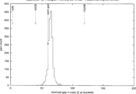
Figure 1 shows a histogram of received packet spacing for a nearly idle path. Figures 3-2 and 3-3 show common histogram shapes we found when run between different RON hosts. Each plot shows measurements for a single path. The histograms here were constructed
Squeezed Pair Histogram: intensity. lcs.mit.edu --> public-burning.lcs.mit.edu 500 M I C 0' o a 0) .I 10 0I 450 400 350 300 C 0 250 200 150 100 50 0 0 50 100 150 200
received gap in usec (2 us buckets)
Figure 3-1: Squeezed Pairs on an idle path. This histogram shows the time between packets at receiver for packets sent 60 /-s apart.
packets at the receiver. The gaps were computed by subtracting the timestamps attached to each probe packet by the receiver's packet filter. Figure 3-3(a) shows pairs that were sent spaced by half the transmission time for a 500 byte packet, and Figure 3-3(b) shows pairs that were sent spaced by half the transmission time for a 1500 byte packet. The long arrow marked 'sent gap' shows the time difference from immediately prior to the send() call for the first probe packet to immediately prior to the send() call for the second probe packet. The sending gaps were chosen dynamically by an online ADR test. Since ADR tests can underestimate capacity, the spacings are somewhat more than half of a transmission time for a 500 or 1500 byte packet. Pathrate was used to measure the path capacity and calculate the narrow link transmission time for 500 and 1500 byte packets.
Pairs plotted that are to the left of the sending gap arrived squeezed at the receiver, and those to the right of the sending gap arrow were spread at the receiver. There are three other arrows on each graph. The leftmost is marked as 'b2b.' This arrow marks the expected arrival gap at the receiver if our probe packets (which are 40 bytes long) exit the narrow link back-to-back and maintain this spacing at the receiver. Pairs may arrive with a spacing smaller than the 'b2b' arrow if the pair were squeezed together after the narrow
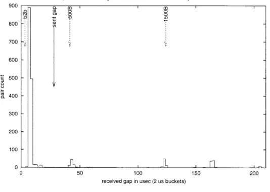
Squeezed Pair Histogram: ccicom. ronics. mit.edu -- > nyu. ronics. mit.edu 02 02 0 0 C C 4) LI) 900 800 700 600 500 400 300 200 100 0 800 700 600 500 400 300 200 100 0 -0 -0 0) C -T-. -0 50 100 150 200
received gap in usec (2 us buckets)
(a) Received gaps when send gap is half the width of a 500 byte packet
Squeezed Pair Histogram: ccicom.ron.Ics.mit.edu -- > nyu.ron.Ics.mit.edu
-C, 0) LP LI) 0
-0 50 100 150 200
received gap in usec (2 us buckets)
(b) Received gaps when send gap is half the width of a 1500 byte packet
Figure 3-2: Typical Squeezed Pair Histograms - A path with queuing on a tight link 0 0 CU) a-:3 0 CU) a CD i i CDA I
n
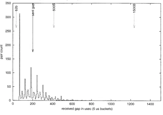
Squeezed Pair Histogram: nyu.ron.lcs.mit.edu --> lulea.ron.lcs.mit.edu n0 c,,j 22 M) Mo
0
200 400 600 800 1000 1200 1400received gap in usec (5 us buckets)
(a) Received gaps when send gap is half the width of a 500 byte packet
Squeezed Pair Histogram: nyu.ron.Ics.mit.edu -- > lulea.ron.Ics.mit.edu
C\J0 0) 0
LO
0 200 400 600 800 1000 1200 1400 received gap in usec (5 us buckets)
(b) Received gaps when send gap is half with width of a 1500 byte packet
Figure 3-3: Typical Squeezed Pair Histograms - A path with queuing on a link faster than
the tight link
0 0 LO 7
link. The arrow marked as '500B' shows the expected arrival gap if the probe packets are spaced by a 500 byte packet on the narrow link. The '1500B' arrow shows the same value for a 1500 byte cross traffic packet.
Figure 3-1 shows a unimodal distribution very close to the sending rate. The most frequently measured gaps at the receiver were between 63 and 65 microseconds, whereas the ideal sending gap was 60 microseconds. The sender and receiver in this test were connected to the same 100 Mbps Ethernet switch, and the machines were mostly idle except for the squeezed pairs test.
In Figure 3-2 only a few packets arrive at the receiver with the same spacing at which they were sent, indicating that there at least one link along the path that is not mostly idle. The other peaks are around 10 ps, 40 ps, 120 [is, and 160 ps. All of the links between ccicom and NYU have a capacity of 100 Mbps or faster. At 100 Mbps, a 1500 byte packet takes 120 ps, and a 500 byte packet takes 40 ps. We therefore assume that packets which arrived at the sender spaced by 40 ps were queued with a 500 byte packet between the two probes. Those that arrived spaced by 120 ps either had one 1500 byte packet or three
500 byte packets between them. The lack of any prominent peak around 80 ps suggests
the former. There is little difference between the histograms of packets sent with a 20 Ps spacing and those sent with a 60 ps spacing. The large mode around 10 As indicates that most pairs were squeezed together, and essentially arrived back-to-back at the receiver. In a separate experiment to determine the accuracy of our timing measurements, we found that the arrival spacing of packets was largely inaccurate with gaps below 20 Ps, though the measured gaps were almost always accurate to within 10 [is when packets were spaced farther apart. As such, the leftmost mode, though twice the 'b2b' rate, is not inconsistent with back-to-back transmission on the tight link.
Figure 3-3 shows almost no overlap between the histograms for the two different sending gaps. In this case, the received gaps are spread symmetrically around the sending gap, with submodes at even intervals. These patterns result when queuing occurs on a faster link along the path than the end-to-end capacity limiting hop. The modes to the right of the sending gap result when the first packet of the pair is queued less than the second. The space between sub-modes can be expressed simply in terms of the size of cross traffic packets. Since there are no packets that arrive with gaps appropriate for cross traffic on the 10 Mbps link, we conclude that all queuing delay occurs on links with capacity higher than 10 Mbps.
This conclusion does not imply that the 10 Mbit hops are idle, merely that they are idle enough that our probe packets are never queued there. We are unsure why the leftmost peak in figure 3-2(a) is roughly double the predicted back-to-back spacing.
Most plots of Squeezed Pair histograms show features in one or both of the non-idle path plots shown. Some do not show distinct sub-modes around the sending gap, but instead show a gradual smear up to a peak at the sending rate. This effect can occur when the the link where queues form is much faster than the capacity limiting link. In this case, the histogram bins are not fine enough to see a single packet gap. Paths where cross-traffic packet sizes are uniformly distributed rather than only a few discrete sizes would cause the same smeared shape.
We have developed a simple scoring program to describe whether or not the histogram modes are symmetric around the sending gaps. Instead of searching for a peak around the sending rate, we check each histogram bin to see whether there is a mode in one or both of the sending rate plots. If a mode appears in both plots, we increment a counter. If a mode appears in only one plot, we decrement the same counter. At the end if the counter is positive, we group that path in those like in figure 3-2, and call these paths tight-like-narrow paths. If the counter is negative, we label the path as tight-unlike-narrow at the time the test was run. For the two paths shown, the path in figure 3-2 scored 1055118, whereas the path in figure 3-3 scored -364009.
We do not claim that these classifications represent the true network state, and in fact know of no general way to identify the true tight link in any path. We use the labels
tight-like-narrow and tight-untight-like-narrow because they are more descriptive than labeling paths as 'sqp+' and 'sqp-', for example. We can construct some simple example cases where the naming fails: consider a path with a narrow link of capacity a, and another link of capacity 2a. If the path is completely idle except for a few cross traffic packets on the 2a link, the true tight link is still the capacity a link, even though squeezed pairs would classify the
Chapter 4
Methodology
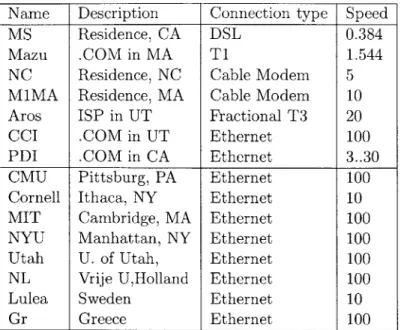
We performed measurements on the RON[5] testbed to compare each of the BTC estimation methods described in chapter 3. The RON testbed currently consists of hosts installed at business, residential, and educational installations. While running our tests, we used fifteen different sites. Three are in Europe, and the remainder are in the US. Table 4.1 lists properties of each host.
We ran tests between successive pair of RON machines at a time. Hosts were picked randomly, with the exception of hosts MlMA and NC. These two hosts were only available for use between 2am and 5am EDT, and thus are underrepresented in the overall sample. Each test proceeded through the phases as follows, and then the same tests were run with the source and destination reversed. We did not perform any measurements during the experiment aside from logging packet departure and arrival times for each test other than the Pathload and Pathrate tests. We discuss calculations needed to process the logs into measurements in section 4.3
4.1
BTC
Tests
4.1.1 Ron probes
The source sends a sequence of 100 UDP packets, on average 10 seconds apart with a random offset of 3 seconds. Each packet is 32 bytes long including IP and UDP headers, and contains only a 32 bit sequence number. The destination echoes each packet back to the source. The whole test takes 16 minutes on average, and sends 3.2 Kilobytes of data,
Table 4.1: RON sites and locations. Bandwidths are in only to the known local Internet access capacity
Mbps. Connection Speed refers
not including link level headers.
4.1.2 Asymptotic Dispersion Rate
The source sends 30 packets back-to-back, pauses for one round trip, and then sends another
30 packets to the destination. Each packet is 1428 bytes long, and includes a sequence
number. The total amount of data sent is 83 Kilobytes. The time for the test varies by link, but would be around 5 seconds for a 128 Kbps path. The test duration on faster paths is usually limited by round trip time rather than the probe packets' transmission time.
4.1.3 Squeezed Pair test
The source sends up to 4000 pairs of packets, with the spacing within each packet set to alternate between half the width of a 500 byte and half the width of a 1500 byte packet based on the path capacity estimate. The pairs are sent with exponentially distributed inter-pair spacings, with a mean space of the larger of ten times the largest intra-pair gap, or 2 milliseconds. Probe packets are 40 bytes long, including IP and UDP headers. The large number of pairs and random spacing was chosen to ensure that received-spacing modes that appear infrequently could be observed. We have not attempted to determine a minimum
Name Description Connection type Speed MS Residence, CA DSL 0.384 Mazu .COM in MA T1 1.544
NC Residence, NC Cable Modem 5
M1MA Residence, MA Cable Modem 10
Aros ISP in UT Fractional T3 20
CCI .COM in UT Ethernet 100
PDI .COM in CA Ethernet 3..30
CMU Pittsburg, PA Ethernet 100
Cornell Ithaca, NY Ethernet 10
MIT Cambridge, MA Ethernet 100
NYU Manhattan, NY Ethernet 100
Utah U. of Utah, Ethernet 100
NL Vrije U,Holland Ethernet 100
Lulea Sweden Ethernet 10
number of pairs to send to ensure that receiver modes are still observable.
4.1.4 Pathload
We use Pathload [17], version 1.0.2. We included a number of local patches to fix bugs, allow operation on paths slower than 1 Mbps, and change the bandwidth resolution parameter to specify a ratio between high and low rates. We ran the modified Pathload with a bandwidth resolution parameter of 0.2, meaning that Pathload tries to report a range where the lower end is no more than 20% below the upper end of the range. We found that this setting allowed Pathload to produce an estimate by testing between 4 and 8 different rates in most cases.
Each Pathload test varies in the amount of data it sends, as it is an iterative algorithm which proceeds by evaluating a number of possible transfer rates. Each rate tested involves 1200 probe packets, broken up into 12 streams each spaced by one round trip time. Each probe packet is at least 200 bytes, for a total cost of at least 234 Kbytes. A typical run that tests 4 different sending rates would source nearly 1 MByte in total probe packets.
4.1.5 TCP test
We send 2 separate TCP bulk transfers from source to destination, one following the other
by one round trip time plus a 5 second delay. In FreeBSD, the largest allowable TCP
window size can be set through the kern. ipc. maxsockbuf sysctl, which we set to allow 1MB socket buffers on both end hosts. We set SO-SNDBUF and SORCVBUF to 1 MB, which causes the receiver to use TCP's window scaling option to advertise a 1 MB receiver window. Each transfer proceeds by placing data into the socket send buffer for 30 seconds. After 30 seconds, if 2 MB of data has not yet been added to the buffer, the source continues sending until 2 MB is sent. In practice, nearly all paths were limited by the 30 second requirement, so the actual amount of data transferred varied widely between paths.
Earlier versions of our TCP test, and also many measurements discussed in the related works, used a fixed transfer size. We found that in many cases the TCP congestion window would not have time to grow large enough to induce any packet losses when sending only a few megabytes of data. A time based approach provides a more accurate base estimate of BTC because we ensure that measurement continues over the course of many round trips.
4.1.6 Capacity Measurements
We ran Pathrate [11] between all pairs of RON nodes. We did not run Pathrate at the same time as all other tests, as a single pathrate run often lasted for as much as twenty minutes, and initially it failed to arrive at a capacity estimate at all on many paths. We found the cause of the failed measurements, namely that pathrate would abort when the last two or three packets of each group, and only those few, were consistently dropped. We repeated pathrate measurements on the paths that exhibited this problem after implementing a fix.
4.1.7 Loaded Paths
In order to ascertain whether the accuracy of various decision metrics depends on how loaded the paths are beforehand, we repeated the sequence of tests above with the addition of an additional ttcp stream between the same source and destination pair. The ttcp stream used the same window sizes and socket buffer sizes as the actual BTC measurement TCP stream. This approach does not display the same features as real cross traffic, since the
competing traffic traverses all of the same links. However, this approach is the easiest way to ensure that the links are not idle.
4.2
Processing
All tests except the Pathload and Pathrate test are captured by tcpdump [25] on both the source and destination. Tcpdump provides timestamps for all packets with a resolution of 1 ps. For received packets this timestamp occurs during the interrupt handler, and for sent packets the timestamp occurs immediately before the packet goes to the Ethernet card. Similar timing data for received packets is available through the use of the SOTIMESTAMP socket option, though tcpdump log processing is more flexible for our purposes. None of our tests require accurate packet timestamps at the source. Measuring gaps at the sender in a tight loop calling gettimeofday( is sufficient for squeezed pairs tests. Although we cannot ensure that the sending process will not be swapped while waiting to send a packet, we can detect pairs with abnormally large spacing at the receiver by filtering out gap sizes that differ greatly from the median value. However, verifying correct operation and processing is easier with logs from both machines. Consequently, any of the methods could be used in an application without requiring the use of tcpdump or libpcap, which implements tcpdump's
interface to the kernel's packet filter.
4.3
From Test Phases to BTC Estimates
In the results chapters we refer to BTC tests by label. Here we describe how BTC estimates for each labeled test are computed.
tcp vs. tcp The tcp vs. tcp metric compares the full transfers on each path. For each of the two bulk TCP transfers, we compute the TCP throughput on the path from the tcpdump traces. The times are computed at the sender, from the time the first SYN packet is sent until the last data packet is sent. Transfer size includes data only, and does not include packet headers or retransmissions. We then treat the throughput of the first connection as a BTC estimate, and the throughput of the second transfer as a BTC measurement to judge the estimate by. We compare the BTC measurement against BTC estimates from
other methods.
short-tcp The short-tcp test is similar to the full tcp test. The difference is that only the first 128 KB (around 90 packets on Ethernet with a 1500 byte MTU) from the first TCP transfer are used to produce a BTC estimate. The full transfer from the second TCP transfer is still used as the BTC measurement to judge the estimate.
adr The ADR measurement phase consists of two groups of 30 packets each. At the receiver, we record the arrival time of each packet, and from this we construct a list of the interarrival times between each successive packet. We then remove the two largest and two smallest interarrival time from each group. We then take the average of the remaining 50 interarrival times, and compute the ADR as L/Atavg, where L is the packet length of each packet including headers, and Atavg is the average spacing.
short adr The short adr is computed in the same manner as the ADR test, but only considers the first 15 packets of each group.
capacity Pathrate reports both an upper range and lower range estimate, corresponding to the size of the bin histograms that pathrate uses. We use the average of these two values as the path capacity.
pathload Pathload reports a range of throughput ranges. The lower range estimate is the highest rate that Pathload found to be below the path's available bandwidth. The upper range endpoint is the lowest tested rate found to be above the path's available bandwidth. Here we consider only the average of the upper and lower end of the range.
RON probes For the RON score comparison, we use the computed score as described in section 3.2.
RON
lossonly
We also show results, labelled as RONlossonly,
for comparisons where atChapter
5
Path Choosing Results
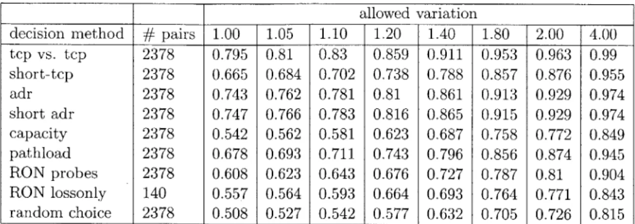
In this chapter we compare the ability of each method to pick between a pair of paths. Tests were conducted between August 5, 2002, and August 12, 2002 for normal (unloaded) paths, and between August 15, 2002 and August 19, 2002 for loaded paths. The tests described in the previous chapter describe the set of packets sent along a path between two RON testbed machines. In this chapter we consider pairs of these of measurements. There is no relation between the time at which one path was measured and the time at which the other path was measured. Since the times (and consequently network conditions) are unrelated, we treat measurements from the same host to the same destination as distinct paths when constructing pairings. We did not use any
forwarding packets through intermediate no
of the RON overlay networks' mechanisms for
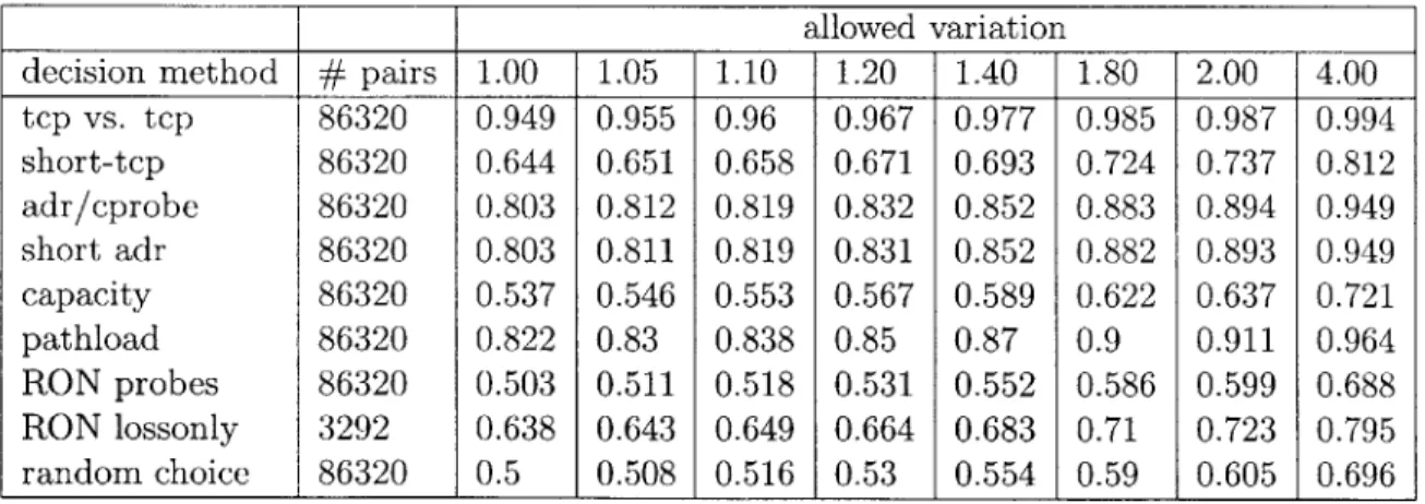
Table 5.1: Correct Decision rates all possible path-pairs allowed variation
decision method
#
pairs 1.00 1.05 1.10 1.20 1.40 1.80 2.00 4.00tcp vs. tcp 86320 0.949 0.955 0.96 0.967 0.977 0.985 0.987 0.994 short-tcp 86320 0.644 0.651 0.658 0.671 0.693 0.724 0.737 0.812 adr/cprobe 86320 0.803 0.812 0.819 0.832 0.852 0.883 0.894 0.949 short adr 86320 0.803 0.811 0.819 0.831 0.852 0.882 0.893 0.949 capacity 86320 0.537 0.546 0.553 0.567 0.589 0.622 0.637 0.721 pathload 86320 0.822 0.83 0.838 0.85 0.87 0.9 0.911 0.964 RON probes 86320 0.503 0.511 0.518 0.531 0.552 0.586 0.599 0.688 RON lossonly 3292 0.638 0.643 0.649 0.664 0.683 0.71 0.723 0.795 random choice 86320 0.5 0.508 0.516 0.53 0.554 0.59 0.605 0.696
5.1
Method Comparisons
To evaluate each decision method, we note whether that metric correctly decides the path with higher BTC for each possible pairing of paths between RON nodes. We use the average throughput of the first of the two bulk TCP transfers as the BTC to decide which path is actually faster. If the method in question chooses the path with higher BTC, then it is counted as a correct choice, otherwise as an incorrect choice. Table 5.1 summarizes the rate of correct choices for each decision metric.
In addition to a strict ordering test, we also examine whether the test decides correctly as long as the BTC values on the two paths are not 'too close' together. We used a range of possible values for the allowed separation ratio. If the ratio of larger BTC to smaller BTC is less than this constant, then the decision metric is counted as correct regardless of which path it chooses. These additional values are relevant for applications that aren't concerned with choosing the best path if the performance of either will be similar, but do care about not choosing a path that is significantly worse than the other.
For example, in Table 5.1, the row labeled tcp vs. tcp describes the correct decision rate where the first bulk TCP transfer is used to predict the second. The column where the separation ratio is 1.0, which shows a correct choice rate of nearly 96%, shows that TCP is consistent on 96% of all path-pairs. The column labeled '1.4' shows that given the results of the first TCP test, there is over a 98% chance that the second TCP test will either agree as to which path is faster, or the BTC of the faster path will be no more than 40% higher than the BTC of the slower path.
We include results for a random choice, labeled random choice, between path pairs for reference. The expected accuracy rate for a random choice is 50% when the allowed variation in BTC measurements is 1.0. When allowed BTC variation is greater than 1.0, the expected accuracy of a random choice depends on the distribution of measured BTC values.
5.1.1 Measurement Costs
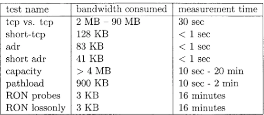
Table 5.2 shows the approximate amount of data and time required for each method to measure a single path. Several of these methods vary the amount of data and measurement times based path conditions as well as parameter settings. In addition, there is room for
Table 5.2: Approximate Bandwidth consumed by each test
efficiency improvements in the implementations. Our purpose in showing these values is to show that measurement costs vary over over several orders of magnitude rather than provide exact values to expect.
5.1.2 All path pairs
First we discuss the most general results shown in table 5.1 and discuss their properties. Later we examine some cases where tests perform poorly and look for correlations between common results for each method. The all-pairs results are useful for applications that wish to rank BTC among a set of Internet paths without regard for whether or not the paths include a given host. One example of such an application would be downloading a large file through an overlay network where you can choose from a set of servers and an intermediate node to transfer through.
Unsurprisingly, the tcp vs. tcp test is by far the most accurate among those we have tried. It is the only test that shows accuracy above 90% in any but the most error-tolerant decision metrics. Several other metrics, short-tcp, capacity, RONprobes, for example, perform poorly even when large variations are allowed in base BTC values. All of these measurements choose the correct pair in less than 75% of pairings, even when we allow a factor of 2 in BTC variation. The RON probes appear little different than random guessing, though matters improve in RON lossonly. Unfortunately, probe losses are quite rare and occur in less than 4% of paths we examined in RON, so we cannot in general choose to use the lossonly test.
Examining the tier of performers just below the tcp vs. tcp test, we find pathload, adr, and short-adr. These tests all miss on the order of 20% of path pairings for exact comparisons,
test name bandwidth consumed measurement time tcp vs. tcp 2 MB - 90 MB 30 sec
short-tcp 128 KB < 1 sec
adr 83 KB < I sec
short adr 41 KB < 1 sec
capacity > 4 MB 10 sec - 20 min
pathload 900 KB 10 sec - 2 min
RON probes 3 KB 16 minutes
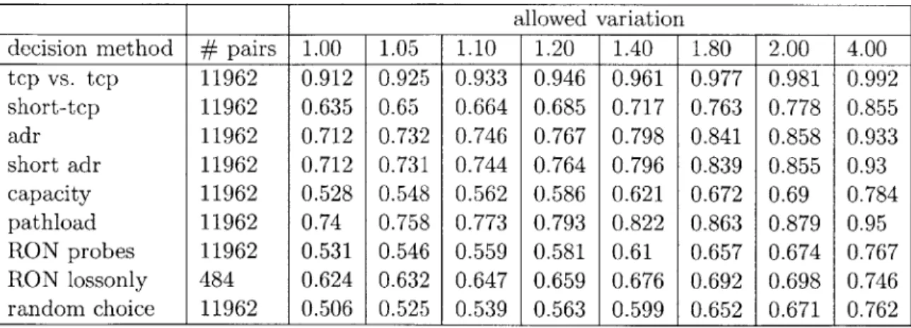
allowed variation
decision method
#
pairs 1.00 1.05 1.10 1.20 1.40 1.80 2.00 4.00tcp vs. tcp 11962 0.912 0.925 0.933 0.946 0.961 0.977 0.981 0.992 short-tcp 11962 0.635 0.65 0.664 0.685 0.717 0.763 0.778 0.855 adr 11962 0.712 0.732 0.746 0.767 0.798 0.841 0.858 0.933 short adr 11962 0.712 0.731 0.744 0.764 0.796 0.839 0.855 0.93 capacity 11962 0.528 0.548 0.562 0.586 0.621 0.672 0.69 0.784 pathload 11962 0.74 0.758 0.773 0.793 0.822 0.863 0.879 0.95 RON probes 11962 0.531 0.546 0.559 0.581 0.61 0.657 0.674 0.767 RON lossonly 484 0.624 0.632 0.647 0.659 0.676 0.692 0.698 0.746 random choice 11962 0.506 0.525 0.539 0.563 0.599 0.652 0.671 0.762
Table 5.3: Correct decision rates for path pairs that share a common endpoint
and only 10% when BTC may vary by a factor of two. The results for the adr test are nearly identical to the short-adr test. This similarity implies that using 60 packets rather than 30 provides little additional value, though we cannot tell from this table whether the two metrics fail on the same or different paths. We address this question in section section 5.3.
The predictive ability of the capacity test are somewhat disappointing. Path capacity changes rarely, and is easy to measure though each measurement is expensive. We speculate on two reasons why capacity estimates are inaccurate. The first is that nearly all paths have a capacity that is one of only a few discrete values, corresponding to popular link types. We can expect capacity estimates only to correctly compare paths that use different physical methods. The second observation is that capacity estimates would perform best if all links operate at loads less than their capacity. We speculate that edge links are often heavily loaded, which makes path capacity an unattractive measurement.
5.1.3 Common Endpoint Pairs
Table 5.3 shows values computed in the same manner as the first table, but is limited to measurements where the two paths shared either a common sender or a common receiver. Here we discuss the differences between these results and the ones for all path pairings. Common endpoint paths are relevant for applications, such as choosing a mirror from which to download a large file, in which only one end of the path may be chosen freely.
In general, the accuracy rate of common-endpoint tests are slightly lower than all pairs tests. For example, the tcp vs. tcp test accuracy declined from 95% to 91%, and other tests