CHARACTERIZATION OF MEASUREMENTS IN QUANTUM COMMUNICATIONS
by
Vincent Waisum Chan
Submitted to the Department of Electrical Engineering on June 25, 1974 in partial fulfillment of the requirements
for the Degree of Doctor of Philosophy. ABSTRACT
A characterization of quantum measurements by operator-valued measures is presented in this thesis. The
'genera-lized' measurements characterized include simultaneous approximate measurement of noncommuting observables. This characterization is suitable for solving problems in quantum communications.
Two realizations of such measurements are discussed. The first is by adjoining an apparatus to the system under
observation and performing a measurement corresponding to a self-adJoint operator in the tensor-product Hilbert space of the system and apparatus spaces. The second realization is by performing on the system alone, sequential measurements
that correspond to self-adJoint operators, with the choice of each measurement based on the outcomes of previous
measurements.
Simultaneous generalized measurements are found to be equivalent to a single 'finer grain' generalized measurement, and hence it is sufficient to consider the set of single
measurements.
An alternate characterization of generalized measurement is proposed. It is shown to be equivalent to the characteri-zation by operator-valued measures, but it is potentially more suitable for the treatment of estimation problems.
Finally, a study of the interaction between the informa-tion carrying system and a measuring apparatus, provides
suggestion for the physical realizations of abstractly characterized quantum measurements.
THESIS SUPERVISOR: Robert S. Kennedy
ACKNOWLEDGMENT
I wish to express my sincere gratitude to Professor
Robert S. Kennedy for his generous guidance and encouragement throughout my years as a graduate student. Under his
super-tision, I have acquired very valuable theoretical and experimental knowledge in the area of communications, and he has provided me with the right stimulation to make this research both interesting and challenging.
I would also like to thank the readers -- Professor Hermann Haus and Professor David Epstein for their valuable suggestions and time in reviewing the manuscript.
My thanks also go to Dr. H.P. Yuen for his valuable discussions and suggestions.
I also want to thank my colleague Sam Dolinar for the many discussions we have had and for reading the manuscript and offering numerous valuable suggestions. Our years of association have been a lot of fun.
Last, but not least, I would like to thank Ms. Agnes Hui for her expert typing and constant encouragement during the course of this research.
Abstract ... Acknowledgment ... Table of Contents ... List o List o PART I CHAPTE CHAPTE CHAPTE CHAPTE CHAPTE ... e...
.. e..ee...eeeeeeo . . . .. eel ee e e.e
eeeeeeeeeeaeeeeaeeeeeeeeeeeeeeeeeee
2
3
II
f Appendices ... .... ... 7
f Theorems and Corollaries 9... 9
CHARACTERIZATION OF MEASUREMENTS IN QUANTUM COMMUNICATIONS ... ... ... 11
IR 1 INTRODUCTION 1.1 Motivation for Research ... 12
1R;2 Introduction to Part I -- the Characteriza-tion of Quantum Measurements ... 13
1.3 Brief Summary of Part I ... 17
1.4 Relation of Part I to Previous Work ... 19
1.5 Introduction and Summary of Part II **... 20
R 2 GENERALIZATION OF QUANTUM MEASUREMENTS --AN INTRODUCTION ... 21
R 3 THEORY OF GENERALIZED QUANTUM MEASUREMENTS ... 25
iR 4 EXTENSION OF AN ARBITRARY OPERATOR-VALUED MEASURE TO A PROJECTOR-VALUED MEASURE ON AN EXTENDED SPACE ... 38
R 5 FIRST REALIZATION OF GENERALIZED MEASURE-MENTS -- FORMING A COMPOSITE SYSTEM WITH AN APPARATUS ... ... .... 45
CHAPTER 6 CHAPTER 7 CHAPTER 8 CHAPTE CHAPTE CHAPTE CHAPTE CHAPTE CHAPTE
PROPERTIES OF THE EXTENDED SPACE AND THE RESULTING PROJECTOR-VALUED MEASURE ... APPARATUS HILBERT SPACE DIMENSIONALITY .... SEQUENTIAL MEASUREMENTS
8.1 Introduction ... 8.2 Sequential Detection of Signals
Trans-mitted by a Quantum System ... 8.3 The Projection Postulate of Quantum
Measurements ... 8.4 The Mathematical Characterization of
Sequential Measurements ... R 9 SOME PROPERTIES OF SEQUENTIAL
MEASURE-MENTS ... ... R 10 SECOND REALIZATION OF GENERALIZED
MEA-SUREMENTS -- SEQUENTIAL MEASUREMENTS ...
R 11 EQUIVALENT MEASUREMENTS ...
R 12 ESSENTIALLY EQUIVALENT MEASUREMENTS ... R 13 SIMULTANEOUS GENERALIZED MEASUREMENTS .... R 14 AN ALTERNATE CHARACTERIZATION OF
GENERALIZED MEASUREMENTS
14.1 Introduction ... 14.2 Another Characterization of Generalized
Quantum Measurements ... 50 62 67 68 74 77 85 90 113 117 133 139 141
CHAPTE PART I CHAPTE CHAPTE CHAPTE CHAPTE CHAPTE
14.3 The Necessary and Sufficient Condition for the Existence of an Extension to
an Observable ... :R 15 CONCLUSIONS TO PART I ... ,1 THE ROLE OF INTERACTIONS IN QUANTUM
MEASUREMENTS ...
:R 16 INTRODUCTION TO PART II ... :R 17 SPECIFICATION OF THE INTERACTIONS
REQUIRED FOR REALIZATION OF QUANTUM
MEASUREMENTS ...
'R 18 THE INTERACTION HAMILTONIAN
18.1 Characterization of the Dynamics of
Quantum Interactions ... 18.2 The Inverse Problem for Finite Duration
of Interaction ... 18.3 The Inverse Problem for Infinite
Duration of Interactions ... :R 19 CONSTRAINTS OF PHYSICAL LAWS ON THE
FORM OF THE INTERACTION HAMILTONIAN
19.1 Introduction ... 19.2 Conservation of Energy ... 19.3 Conservation of an Arbitrary Quantity ... 19.4 Constraints of Superselection Rules ... .R 20 CONCLUSIONS TO PART II ... 144 147 149 150 156 164 170 177 180 181 187 190 193
APPENDIX
A
APPENDIX B
APPENDIX C
APPENDIX D
APPENDIX E
APPENDIX F
APPENDIX G
APPENDIX
H
APPENDIX IAPPENDIX
J
APPENDIX
K
APPENDIX L
APPENDIX
M
APPENDIX
N
APPENDIX OStatement of Theorem for Orthogonal Family of
Projections .
...
194.
Spectral Theorem ...
195.
Naimark's Theorem
.
...
196.
Proof of Theorem 4.2 ...
202.
Proof ot Theorem 4.3 ...
209.
Proof of Theorem 6.1 ...
211
Proof of Theorem 6.2
.
...
214.
Proof of Theorem
6.3
...
219
Proof of Corollary 6.3 ...
227.
Sequential Detection of Signals Transmitted
by a Quantum System (Equiprobable Binary
pure state) ...
23 0
Proof of Theorem 10. 1 ... . 236.Proof and Statement of Theorem 10.2 ...
246.
Procedure to Find the 'FINEST' simultaneous
invariant subspaces of a Set of Bounded Self-adjointOperators ...
249.
Proof of Theorem 12.3 ...
255.
APPENDIX P ... ... 267.
APPENDIX Q Stone's Theorem ...
270.
References ...
271
Biographical Note ... 274
Theorem
3.1
......
...36
Theorem 4.1 . ... ... 38 Theorem 4.2 ... ...5...
40 Theorem 4.3 ... 42 Theorem 3.1 (a) ... 48 Theorem 6.1 ... 55 Theorem 6.2 ... 56 Theorem 6.3 ... 57 Corollary 6.1 ... .. ... 57 Corollary 6.2 ... . ... ... 58 Corollary 6.3 ... ... 58 Theorem 7.1 ... ... ... 62 Theorem 7.2 ... 63 Theorem 7.3 ... ... 64 Theorem 7.4 ... ... 65 Theorem 9.1 ... ... 86 Corollary 9.1 ... 87 Corollary 9.2 ... 88 Theorem 9.2 ... . ... . 89 Theorem 10.1 ... . ... 91 Corollary 10.1 .. ... ... ... 94 Corollary 10.2 ... ... 94 Theorem 10.2 ... 94 Theorem 10.3 ... ... 95 Corollary 10.3 ... ... 101Theorem 10.4 . ... *... 108 Theorem 10.5 ... ... 111 Corollary 11.1 ... 115 Theorem 12.1 .... ... ... 117 Theorem 12.2 ... ... ... 125 Theorem 12.3 ... 128
Theorem
13.1
...
...
...
135
Theorem 13.2 ... 137 Theorem 14.1 ... 144PART I
CHARACTERIZATION OF MEASUREMENTS IN QUANTUM COMMUNICATIONS
CHAPTER 1 INTRODUCTION
SECTION 1.1 Motivation for Research
Recent developments in coherent and incoherent light sources, optical processors, detectors, optical fibers, etc. have sparked wide interests in optical communication systems and optical radars. At optical frequencies, quantum effects can be very significant in the detection of signals. In fact, there are many cases where quantum noise completely dominates other noise sources in limiting the performance of optical systems. In order to design, and to evaluate quantum optical systems, it is essential to have a good understanding of the properties of quantum measurements. It is the purpose of this thesis to present a characteriza-tion of quantum measurements which the communicacharacteriza-tion
engineers will find convenient to use. The study of the interaction between the information carrying system and a measuring apparatus, provides a suggestion for the physical realization of abstractly characterized quantum measurements.
SECTION 1.2 Introduction to Part I -- the Characterization of Quantum Measurements
It is a general assumption in quantum mechanics that a measurement on a quantum system is characterized by a self-adjoint operator, also known as an observable. Usually, the Hilbert space in which this self-adJoint operator acts, is not well defined. And in some literature it is not even
mentioned. Frequently, one assumes that the Hilbert space is the one that includes all (but only) the accessible states of the system. That is, it is possible to put the system in
any given state in this Hilbert space. Occasionally, one can make use of the a priori knowledge of how the quantum system has been prepared, and specify the Hilbert space as the one that is spanned by the set of states that occur with non-zero a priori probabilities. Only rarely is the Hilbert
space considered as any one that includes the set of acce-ssible states as a proper subspace. And it is only in such a definition of the Hilbert space that every measurement is
characterized by a self-adJoint operator. However, this definition of the space is often unacceptable, because one
is seldom sure how big the Hilbert space has to be before a particular measurement can be characterized by a
self-adjoint operator within the space. It is particularly
the optimal measurement, by optimizing over a set of such loosely and poorly defined measurements. Therefore, the communication engineer is interested in characterizing the set of all quantum measurements by operators acting in more well-defined Hilbert spaces, such as the space spanned by all the accessible states, or the space spanned by the set of states with non-zero a priori probabilities. When
defined on such spaces, not every measurement can be charac-terized by a self-adJoint operator. For example, Louisell and Gordon [1], and recently Helstrom and Kennedy [2] and Holevo [3] have noted that if the system under observation is adjoined with an apparatus, and a subsequent measurement is performed on both systems, the scope of measurement can be extended to at least simultaneous approximate measurements of noncommuting observables. This particular type of measure-ment is important because it has been shown [2] that minimum Bayes Cost in communication problems may sometimes be
achieved by such measurements. The several authors noted above, have suggested that the characterization of quantum measurements by operator-valued measurements is appropriate
for quantum communications. Yuen [4], and then Holevo [3] have derived necessary and sufficient conditions on the
operator-valued measures for optimal performances in detection problems. It seems then, this characterization of measurement is at least useful in calculating optimal performances of
quantum receivers. However, being essentially an abstract mathematical characterization, it does not suggest how the measurement can be realized physically. Furthermore, it does not explain what happens to the system as a result of the measurement. This is in contradiction to the self-adjoint observable view of quantum measurement, where the observable can be expressed as a function of a set of genera-lized coordinates of the system and one can at least see
what coordinates of the system the measurement should measure in some fashion. Also the von Neumann Projection Postulate
(see Chapter 8) gives the final state of a system after a self-adjoint measurement. So there are nice properties about a self-adjoint observable that are better than the operator-valued measure approach, particularly when one is interested in physical realization of quantum measurements. An observable is usually considered to be physically
measurable, at least in principle, while there has been
no indication at all that any measurement characterized by an operator-valued measure can be measurable at all, even in principle. But it is very important for a communication engineer to optimize his receiver performances on a set of measurements that is at least physically implementable in principle. Recently Holevo [3] has noted that for every operator-valued measure, one can always find an adjoining apparatus and a self-adJoint observable on the composite
system, such that the measurement statistics is the same as given by the operator-valued measure. In Part I of this thesis, we show, given the operator-valued measure, how the apparatus Hilbert space can be found and what the corres-ponding observable is. This constructive procedure, we will call our 'first realization of generalized measurements'.
The method described is not the only way to realize a
generalized measurement however. If one considers a sequence of self-adjoint measurements performed on the system alone, the statistics of the outcomes sometimes correspond to those given by an operator-valued measure. This, we call our
'second realization'.
Since considerations of simultaneous measurement of noncommuting observables lead to the operator-valued measure characterization, we will consider the simultaneous measure-ment of two or more measuremeasure-ments characterized by operator-valued measures.
Finally, we propose an alternate (but equivalent)
characterization of generalized measurements. This charac-terization is potentially very useful in considering
SECTION 1.'3 Brief Summary of Part I
In Chapters 3 and 4, we address the mathematical problem of the extension of operator-valued measures to
projector-valued measure on an extended space. (The results are used only in the proofs of the theorems in later chapters. For a general appreciation of the results of this thesis,
Chapter 4 can be skipped). The first realization of genera-lized measurement by adjoining an apparatus is described in Chapter 5. In Chapter 6, several properties of the extended space and the resulting measure are discussed. The dimen-sionality results are used in Chapter 7 to determine the dimensionality of the apparatus Hilbert space required for the first realization. They are also used in the 'second' realization of several classes of generalized measurements by sequential measurements, which is developed in Chapters 8 and 9 and the main results given in Chapter 10. Although not every operator-valued measure corresponds to a sequential measurement, we have.been able to show in Chapters 11 and 12 that a large class of measurements in quantum communications can be realized by sequential measurements with the same or arbitrarily close performances.
In Chapter 13, we show that a simultaneous measurement of two or more generalized measurements corresponds to a
single generalized measurement. Hence, consideration of such measurements will not give improved performances.
Chapter 14 gives an alternative characterization of generalized measurements.
SECTION 1.4 Relation of Part I to Previous Work
Holevo suggested the realization by adjoining an apparatus, when he noted Naimark's Theorem provides an extension of operator-valued measures to projector-valued measures on an extended space [3]. The method of embedding
the extended space in the tensor product space of the system and apparatus is found by the author.
P. A. Benioff has done some work in the area of sequen-tial measurements, 51, [61, [71 at the same time of this thesis research. The characterization of sequential measure-ment is similar to that given in Chapter 8.
SECTION 1.5 Introduction and Summary of Part II
Although self-adJoint observables can in principle be measured, very few of them correspond to known implementable measurements. In Part II, we will show, how by means of an interaction between the system under observation and an apparatus, the relevent information can be transformed in such a way that by measuring a measurable observable, we can obtain the same outcome statistics of the abstractly charac-terized measurement. Chapter 17 shows what type of trans-formation is required and Chapter 18 provides means to find the required interaction Hamiltonian. Inferences as to what coordinates of the system and apparatus should be coupled together and in what fashion, are drawn. Then in
Chapter 19, the constraints of physical law on the 'allowable' set of interactions are discussed.
CHAPTER 2
GENERALIZATION OF QUANTUM MEASUREMENTS AN INTRODUCTION
It is generally assumed in quantum mechanics that an observable of a quantum system is characterized by a self-adJoint operator defined on the Hilbert space which describes the state of the system. Let us call this operator K, and assume it has a complete set of orthonormal eigenvectors
{Iki>}iei, associated with distinct eigenvalues {kil}i¢l
where I is some countable index set, and,
Klki> = kilki> (2.1)
Each commuting and orthogonal projection operator
{Hi - Iki><kiJ}ie projects an arbitrary vector of the
Hilbert space into the subspace spanned by Iki> and together they form a complete resolution of the identity, that is,
AI
i = I (2.2)where
I
is
the
identity
operator
where I is the identity operator.
performed, one of the eigenvalues ki will be the outcome and the probability of getting ki is,
P(ki) = <sinils>, (2.3)
if the system is described by a pure state Is>, or,
P(ki) = Tr{Ps1l i }, (2.4)
if the system is described by the density operator p s
This formulation of the measurement problem does not include all possible measurements. For example it does not encompass a simultaneous measurement of noncommuting observa-bles. Louisell and Gordon [1] and recently Holstrom and Kennedy [2] and Holevo [3] have noted that if the system S
is made to interact with an apparatus A and subsequent measure-ments performed on S+A or A alone, the scope of measurement
can be extended to at least simultaneous approximate measure-ments of noncommuting observables of S. In particular, one
can perform measurements corresponding to a set of noncommuting, nonorthogonal self-adJoint operators {Qi}icl, defined on HS
the system Hilbert space, which forms a resolution of the identity in HS.
I Qi = I (2.5)
To illustrate this possibility we consider the interaction of the system S with an apparatus A. Before interaction the Joint state of S+A can be represented by the density operator
to = to to (2 .6)
PS+A PS A
defined on the Tensor Product Hilbert space HS ® HA = HS+A
where denoted tensor product. The result of the interaction is a unitary transformation on the oint state. At any
arbitrary time t later than to, the density operator of the combined system and apparatus is,
pt = tU(tto)ptO o pOut(t,to ) (2.7)
PS+A ' S A
where U(t,to) is the said unitary transformation.
Let {i(t)}iel be a set of commuting, orthogonal projectors in HS® HA at the time t. If we perform a
measurement characterized by the i' s, the probability of getting the eigenvalue ki corresponding to the subspace which ni projects into, is
P(ki) = Tr{p +Ai(t ) (2.8)
The {Ri(to))ic! again form a commuting, orthogonal projector-valued, resolution of the identity in HS$ HA, and
P(ki) = Tr{p to ptoi(to)} (2.10)
Defining Q TrA{Ptoll(to). (2.11)
where TrA indicates taking partial trace over HA. We obtain
P(ki) = TrS{PSQi} (2.12)
where TrS indicates taking trace over HS.
The set {Qi}is! is again a resolution of the identity but in general the Qi's are not orthogonal, nor commuting and furthermore, they only have to be nonnegative definite self-adJoint operators. However, it can be easily shown that if the Qs are projectors it is necessary and sufficient that they are orthogonal (A statement of the theorem due to Halmos is given in Appendix A). This particular form of measurement is important because it has been shown that minimum
Bayes Cost in the communication problems may sometimes be achieved by such measurements.
CHAPTER 3
THEORY OF GENERALIZED QUANTUM MEASUREMENTS
We will now specify a generalized theory of quantum measurements, that does not necessarily correspond to
measurements characterized by self-adJoint operators on the Hilbert space that describes the system under observation.
As we have noted in the last chapter, in quantum mechanics, an observable is characterized by a self-adJoint operator K
which possesses a set of orthogonal projection operators { i} such that
Ski
=I.
i
The set of projection operators are said to form a commuting resolution of the identity, and defines a projector-valued measure on the index set {i}.
Due to the inconvenience of this characterization of quantum measurements to take into account of simultaneous approximate measurement of noncommuting observables, it is necessary to consider more generalized measurements
characterized by 'generalized' resolutions of the identity.
The requirement on the i's being projection operators is relaxed, by replacing i's with nonnegative definite operators Qi's, having norms less than or equal to one, so
Cs iJi I.
Now the 'measurement operators' Qi's no longer have to pair-wise commute, nor are they orthogonal to each other in
general. The Qi's then define an operator-valued measure on the index i.
Sometimes, the resolution of the identity does not have to be defined on countable index sets like the integers.
For example the index set can be the whole real line. In the next few pages, we will discuss more general definitions of
resolutions of the identity. Some of the terminologies will be required for the discussion of estimation problems, although for detection problems, what is given above is generally
adequate.
* See references [9], [10],[11] for more detailed motivations and discussions.
DEFINITION. A resolution of the identity is a one parameter family of projections {Ex<} X<+ which satisfies the following conditions,
(i)
EkE = Emin(A,)(ii) E o -= 0, E+ = I,
(iii) EX+ 0 - EX
where E+0x = Ji EX
E+O x = 1$ E x,
x is an element in the space H. (3.1)/
Such a family of operators defines a projector-valued measure on the real line R. For an interval A (X,1X2], where X1<X2, the measure E(A) E E2-EX1 is a projection
operator (thus the name). It follows from condition (i) that for two disjoint intervals A1,A2 on the real line,
E(A 1)E(A 2) = 0. (3.2)
arbitrary disjoint subsets of the real line (see Appendix A). In this sense the resolution of the identity EX is also
called an orthogonal resolution of the identity.
For a small differential element d, the corresponding measure is dE. = E(dX) = E+dX-E .
The integral
A = flXdEX (3.3)
converges in strong operator topology, and defines a self-adjoint operator in the Hilbert space H. Conversely, by the Spectral Theorem for self-adjoint operators (see Appendix B), every self-adjoint operators possesses such integral repre-sentation. The family {Ex} is called the spectral family for the operator A.
Sometimes the projector-valued measure is defined on only a finite number of discrete points, (for example the points may be the integers i = 1,...,M) and it is often more convenient to write the measure Hi corresponding to each point i explicitly. The measures { i} are projection
Ci n = I (3.4)
The orthogonality condition in equation (3.1) becomes,
Bidj = 6ijEj (3.5)
where 6ij is the Kronecker 6-function 6ij = {o i='J
To reconstruct the resolution of the identity given in the definition, one only has to define,
X)
= I Ili (3.6)
i's
and {Ed} will have all the desired properties of a resolution of the identity.
EXAMPLE 3.1
If a self-adJoint operators A has a set of eigenvectors {lai>}i=l that forms a complete orthonormal basis for the Hilbert space H, then A can be written as,
M
A =
i
I ailai><ail (3.7)The set of projection operators,
Hi = lai><ail (3.8)
forms a projector-valued measure on the integers, i 1,...,M, and they sum to the identity operator.
M
I ri = I (3.9)
i=l
DEFINITION. A generalized resolution of the identity is a one parameter family of operators {F } _.<x<+ . which satisfy the following conditions,
(i) if 2>1, F 2-F 1 is a bounded nonnegative definite
operator (which implies it is also self-adJoint.) (ii) FX+ F1
(iii) F_ = 0, F+ = I. (3.10)/
Such a family of operators defines an operator-valued measure on the real line. For example, if we have an interval
A = ( 1,A2], where 1 Ax2, the measure is F(A) = FX2-F 1. For a small differential element d, the corresponding measure is dF = F(dX) = F +dX-F . Whenever the integral
A = fIdFl converges in strong operator topology, it defines a symmetric operator A in the Hilbert space H (i.e. its
the family {Fa} is called the generalized spectral family for the operator A.
A projector-valued measure is a special type of operator-valued measure. However operator-operator-valued measures are more
general in the sense that the measures are nonnegative definite self-adjoint operators instead of being restricted to projec-tion operators only, as is the case in projector-valued
measures. One of the consequences of this definition of
measure is that the measures of two disjoint subsets of the index set do not have to be orthogonal as in projector-valued measures.
EXAMPLE 3.2
An example of operator-valued measures that is not a
projector-valued measure is when {El}, {El} are two projector-valued measures that do not commute for at least one value of X, and we form the generalized resolution of the identity,
FX = E + (-a)E X (3.11)
where a is a real parameter in the interval (0,1). Specifical-ly, FX defines an operator-valued measure, but not a
As in the case of projector-valued measure, sometimes an operator-valued measure is defined on only a finite number of discrete points (for example, the points may be the integers, i = 1,...,M) and it is more convenient to write the measure Qi corresponding to each point i explicitly. The measures Qi's are nonnegative definite self-adJoint operators with norm less than or equal to one. To reconstruct the resolution of the identity given in the definition, one only has to define
F = I Qi (3.12)
i<Ai
and {Fx} will have all the desired properties of a resolution of the identity.
EXAMPLE 3.3
Figure 3.1 shows three vectors Isi>, i=1,2,3 with the symmetry that <s is > - / for all i. (3.13)
Is2
> 120 1200 53>Figure 3.1
If we define = lsi><sil, i = 1,2,3 (3.14) i 3 Then Qi = (3.15)
i=l
and Q (3.16) SoQ} i iSo {Qi}i= is an operator-valued measure but not a
projector-valued measure, on the space spanned by the {Isi>}.
The operator-valued measure {Qi above is defined on the real line R. One can also define operator-valued measures on general measurable spaces.
If (X,A) is a measureable space (where X is the space, and A a collection of subsets of X, on which an appropriate measure can be defined (for example, A can be a a-algebra, a-ring, a-field, and so forth); a map F(.) can be defined as follows,
For all subsets AcA, A F(A), where,
(i) F(A) is a bounded nonnegative definite self-adjoint operator,
(ii) the map F(.) is countably additive, i.e. for any countable number of pairwise disjoint subsets in A, {Ai} say,
F( VAi) = I F(Ai), (3.17)
i
(iii) F(X) = I, the identity operator in H, so F(.) is
a resolution of the identity, (iv) for the null set 0, F(0) = 0./
EXAMPLE 3.4
The output of a laser well above threshold is in a coherent state 151 A coherent state a> is labeled by a complex number a, where the modulus corresponds to the
amplitude of the output field, and the phase of a corresponds to the phase of the field. The inner product between two coherent states
Ia>,1>
is given by,al
= expa a- 2a
-
81
2 (3.18)The coherent states can be expressed as a linear combina-tion of the photon states In>, n = ,1,... where the integer n indicates the number of photons in the field
la> = e l/21 (n!)l ln (3.19)
The Hilbert space H that describes the field is spanned by the set of photon states {In>}n0 and,
n=Oand
(3.20)
XI n><nl = I. H n=O
If we define
{IIn = In><nl n=O
n ~n=O (3.21)
The set of projectors { n } is a projector-valued measure defined on the positive integers of the real line.
The set of coherent states also spans H, and the integral
fcla><ald2a = IH (3.22)
where C is the complex plane and d2a c dIm(a)dRe(a). If we define
{Q = la><a }aeC (3.23)
we have an operator-valued measure {Q a} defined on the complex plane C instead of the real line and
so it is not an orthogonal resolution of the identity.
A measurement on a physical system can be characterized by an operator-valued measure, with the outcome of the measure-ment having values in (or labeled by elemeasure-ments in) X. The
probability of the outcome falling within a subset AcA, is given by Tr{pF(A)}, where p is the density operator for the system under observation. When a measurement is characterized by a single self-adJoint operator, sometimes called an
observable, the measures are all projector-valued. Here, the measures are generalized to nonnegative self-adJoint operators with norms less than or equal to one. A natural question that arises is, how do we realize such generalized measurements. Does every operator-valued measure corresponds to some physical measuring process? In the sequel we will prove the following major theorem.
THEOREM 3.1
Every operator-valued measure can be realized as corresponding to some physical measurement on the
quantum system under question in the following sense, (a) it can always be realized as a measurement
corres-ponding to a self-adJoint operator on a composite system formed by the system under observation and
or,
(b) under suitable conditions which will be specified later, it can be realized as a sequence of
self-* adJoint measurements on the system alone. /
In conclusion to this chapter we will give a simple example where
an observable cannot provide the type of information we desire and
generalized measurements have to be used.
Consider the situation when the information to be transmitted is
being stored in the orientation of the spin of an electron.
The
electron
will be in one of three possible states, just as those described in Example
3.3. By performing a spin measurement on the electron (that is, a
Stern-Gerlach type experiment), one can only have one of two possible
outcomes. This measurement is clearly unacceptable for distinguishing
between three possibilities.
It is then necessary to bring in an apparatus
to interact with the electron and the subsequent measurement done onthe compoiste system will give the desired outcome statistics.
* We will restate this theorem in more precise mathematical
CHAPTER 4
EXTENSION OF AN ARBITRARY OPERATOR-VALUED MEASURE TO A PROJECTOR-VALUED MEASURE ON AN EXTENDED SPACE
This chapter entirely concerns the proof of Theorem 3.1 and actually provides two construction procedures for the extension space and extended projector-valued measure. For those readers, who neither are interested in the proof nor the construction, this chapter can be skipped without major difficulties later in understanding the thesis. Example 4.1 then may be very instructive to read.
In order to prove Theorem 3.1 we need some preliminary mathematical results. First we like to investigate the extension of an arbitrary operator-valued measure to a
projector-valued measure on an extended space. Two slightly different methods of extension will be given, since each has its own merits and usefulness.
Holevo has noted that Naimark's Theorem provides such an extension
THEOREM 4.1 NAIMARK'S THEOREM
for the space H. Then there exists a Hilbert space H which contains H as a subspace, and there exists an
orthogonal resolution of the identity Et for the space
H+, such that Ftf = PHE f, for all feH, where PH is the
projection operator into H./
The proof, which provides an actual construction, is given in Appendix C.
The second method of extension is related to the unitary representations of *-semigroups.
DEFINITION. Let G be a group. A function T(s) on G whose values are bounded operators on a Hilbert space H, is called positive semi-definite if T(s- 1 ) = T(s)t, for every sG and
CI {T(t-ls)h(s),h(t)} > 0 (4.1)
seG tG
for every finitely nonzero function h(s) from G to H,
(that is, h(s) has values different from zero on a finite subset of G only)./
DEFINITION. A unitary representation of the group G is a function U(s) on G, whose values are unitary operators
on a Hilbert space H, and which satisfies the conditions, U(e) = I (e being the identity element of G), and
U(s)U(t) = U(st), for s,teG./
The following theorem is due to Sz-Nagy [12].
THEOREM 4.2.
(a) If U(s) is a unitary representation of the group G in the Hilbert space H , and if H is a subspace of H , then T(s) = PHU(s)/H is a positive definite function on G such that, T(e) = IH. If moreover, G has a topology and U(s) is a continuous function of s (weakly or
strongly, which amounts to the same since U(s) is
unitary), then T(s) is also a continuous function of s.
(b) Conversely, for every positive definite function T(s) on G, whose values are operators on H, with T(e)=IH, there exists a unitary representation of G on a space H+ containing H as a subspace, such that
T(s) = PHU(s)/H for sG, (4.2)
* / means the operatorsis restricted to operate on elements in H.
and the minimality condition for the smallest possible f , i given by,
H+ = GU(s)H * (minimality condition) (4.3)
This unitary representation of G is determined by the function T(s) up to an isomorphism so that one can call it "the minimal unitary dilation" of the function T(s). If moreover, the group G has a topology and T(s)
is a (weakly) continuous function of s, then U(s) is also a (weakly, hence also strongly) continuous function of s./
The proof, which also involves a construction, is given in Appendix D for easy reference.
Given Theorem 4.2, one can easily arrive at the following theorem for the extension of arbitrary operator-valued measures.
* U(s)H means the set of all elements U(s)f, for all fH. AMJ is defined as the least subspace containing the family of subspaces {Mj).
** An isomorphism between two normed linear spaces H1 and 2
is a one-to-one continuous linear map M : H1 + H2 with MH 1 = 2'
THEOREM 4.3.
Let {Fk} be an operator-valued measure on the interval 0 < X < 2, then there exists a projector-valued measure Ek} in some extended space H+= H such that F = PHEX/H for all ./
The proof is given in Appendix E.
Note that the minimality condition of Theorem 4.2
a H = V U(n)H (4.4) n=O is equivalent to H+ = VE H (4.5) XX
and the system (H ,{E } ) is determined up to an isomorphism. Also the interval of variation of the parameter X, [0,2w) can be extended to any finite or infinite interval by using a continuous monotonic transformation of the parameter X.
EXAMPLE 4.1. [31]
In Example 3.3 we give an operator-valued measure that is not a projector-valued measure. Three vectors {Isi>}3= have the structure shown in Figure 4.1. If we define,
Is2
>1>
-/7f
Fig.4.1 Possible states Fig.4.2 Configurations of
of S. n i =
kfi><
1il2.s>
il,2,3
(4.6)
Qi = 3i i><sil i=1,2,3
Then, C = I (4.7)
iIlQi
=I
where IH denotes the identity operator of the two dimensional Hilbert space H spanned by the three vectors {Isi>i=l . Pick
any extra dimension orthogonal to H to form H+ together with H. Let {lIi>i=1l be an orthonormal basis for the three
dimensional space H+ as shown in Figure 4.2. By symmetry considerations, we adjust the axis of the coordinate system made up of the {(li>}3l to be perpendicular to the plane H spanned by the (Isi>). The projections of the oi>'s on the plane of the Isi>'s along the axis are adjusted so that they coincide with their respective si>, so that <$ilsi> =constant for all i, is maximized (see Figure 4.2). By straight-forward
_-geometric calculations
v< ils>,12 2
and
PHi
>= Isi>.
Hence
PHI i><~ilPH 2= si><si
= PH1HiPH for all i
where i Iyi><~il for all i, and
i
= I +.
(4.11)
i=l H
Therefore, {I i) is the projector-valued extension of {Qi} on
the extended space H
+.
(4.8)
(4.10)
= QiCHAPTER 5
FIRST REALIZATION OF GENERALIZED MEASUREMENTS -FORMING A COMPOSITE SYSTEM WITH AN APPARATUS
Given Theorems 4.1 and 4.3, we can immediately prove part (a) of Theorem 3.1. However we will first define some
mathematical quantities in order to state the Theorem more precisely.
When we combine two systems, S and A say, together to form a composite system, and if Hs and HA are the respective Hilbert spaces that previously describe their individual
states, then the oint state of S+A can be described by the Tensor Product Hilbert Space HS HA formed by the tensor product of the two spaces Hs and HA. Thus if the state of S is Is> and the state of A is a>, in the absence of any interaction between S and A the oint state of S+A is denoted by Is>la>. Moreover every element in HS® HA is of the form,
E cilsi>lai>,
* Holevo has suggested this procedure in a former paper [3] though a detail development was absent.
where the ci's are complex numbers such that 1Ici12<oo, and the
i i
Isi>'s and lai>'s are elements in HS and HA respectively.
The inner product on HS HA is induced in a unique way by the inner products on the constituent spaces HS and HA,
so that,
(<all<sll,IP 2>la 2>) = <lls 2><a11a2> (5.1)
It is an immediate consequence of the above structure for the tensor product space HS® HA that if we have a set of complete orthonormal basis for each of the two spaces HS and HA then the set of tensor products of the elements in these two sets, taken two at a time, one from each set, forms a complete orthonormal basis for HS ® HA' That is if {Isi>)ie! and
{laj>)jeJ
are sets of complete orthonormal basis for HSand HA respectively, then the set {Isi>laj>}iI, jeJ forms a complete orthonormal basis for the space HS HA cannot be separated into the tensor product of an element in HS and an element in HA but it is possible to express every element in HS @H A as a linear combination of elements that are separable.
Given the above definition of the space HS0 HfA' the operators in this space can easily be defined. If TS and TA are bounded linear operators in HS and HA respectively, then
there is a unique bounded linear operator TS0 TA in HS HA with the property that
(TS TA)(Is>Ia>) = (TsIS>)'(TAla>) (5.2)
for all Is>eHS, and all la>eHA.
TS TA is called the tensor-product of the operators TS and TA. Thus if the state of S is described by the density operator pS and A by PA' one can show in the absence of inter-actions, the Joint state is given by the operator PS0 PA' By linearity the operation of the operator TS0 TA can be extended to arbitrary elements in HS0 HA. Again the most general operator on HS® HA cannot be written in the form of the tensor product of two operators as above, but they can
be expressed as a linear combination of such product operators, and linearity defines their operations uniquely on elements in HS HA
It is obvious that the above description can be extended easily to describe a composite system with arbitrarily many (but finite), instead of two, component systems.
This concludes, for the moment, the characterization of composite quantum systems. We will discuss the dynamics of
such systems later when we talk about interactions.
Now we are able to state Theorem 3.1 (a) more precisely.
THEOREM 3.1 (a)
Given an arbitrary operator-valued measure {Q }aA' where A is one index set on which the measure is defined,
one can always find an apparatus with a Hilbert space HAP a density operator PA, and a projector-valued measure {Ha csA corresponding to some self-adjoint operator
= q on HSOHA such that the probability of A'
getting a certain value q corresponding to Qa as the outcome of the measurement, is given by,
P(q ) = TrS{PSQ a
TrS+A{PS® PAnl} (5.3)
for all density operators pS in HS; where TrS is the trace over HS and Trs+A the trace over HS@HA./
* The trace of an operator D over a space H is defined as Tr{D}=I<filDIfi>, where {Ifi>} is any complete orthonormal basis of H.. This quantity is independent of the particular choice of basis.
Proof.
We already know from Theorem 4.1 and 4.3 that an arbitrary operator-valued measure {Q }caA with operator-values on the space HS can be extended to a projector-valued measure {alae A
with operator-values on an extended space H + that contains HS
as a subspace. H+ can be embedded easily in a tensor product space HS® HA for some apparatus Hilbert space with enough dimensions. We will address the question of how many dimen-sions are required, later. Assume, for the moment, that HA has enough dimensions such that the dimensionality of the space
HS® HA is greater than or equal to that of H+. If the state
of the apparatus is set initially at some pure state la>, then the oint state of +A can be described as the tensor product PS la><al of a density operator pS in HS and the density operator PA = la><al in HA. Hence for every element Is> in
Hs it can be identified as the element Is>la> in HS0 HA. And the whole space HS can be identified as the space HS$ Mla> where Mla> is the one dimensional subspace of HA spanned by the element a>. Now H = HSa MIa> is a proper subspace of HS ®HA. The projection operator into the subspace H can be identified as PH = Iffs® la><al where the set {Isi> } is any orthonormal basis in Hs. We can form an operator-valued
measure {Qa ela><al} zA with values in the space H. By Theorem 4.1 and 4.3 there exists a projector-valued measure
{I}a I A on an extended space H+, which we can take as HS HA
since we have assumed that H
A has enough dimensions, such that,
Qa a><al = PHllaPH, for all acA.
Now for an arbitrary density operator PS in HS,
Trs{ SQa} = TrS+A{(PS ® I a><al )(Qa ® a><al )}
= TrS+A{(PS Ia><al )PHIIaPH}
Using the relation, T
Trs{ PSQa }
But
® l a><a
r{BC} = Tr{CB},
= TrS+A{PH(PS @ la><al )PHII}.
is an operator PH(PS lIa><al)PH = in H. PS @ la><al. Therefore, Trs{PsQ } = Trs+A{PSI la><a lI },
for any arbitrary density operator pS./
Note, Q = <a (Qa la><al)la>
(5.5)
(5.6)
Hence,
(5.7)
= TrA{ (Qa I a><al )(IHS la><al )} = TrA{ (PHa PH ) P } = TrA{PHaPH } = TrA{PH a} = TrA{(IH I a><al)n a } Sa
= TrA{ (IHS PA )II a }
where TrA denotes partial trace over the space HA.
(5.9)
*
EXAMPLE 5.1
We will make use of the operator-valued measure described
* The partial trace of an operator D in H H A over the apparatus Hilbert space HA is defined as the operation
i
Isj ><ai
<sj
ID sj,>
ai><ssj
Iwhere {Isj>}, {ai>} are complete orthonormal bases in HS and HA respectively.
--in Example 3.3 and 4.1, In Example 4.1 we have already found the projector-valued measure extension {ii3= in the
three-i three-i=l
dimensional extended space H . If we consider the original two-dimensional Hilbert space H as the system space HS, all we have to do is to find an apparatus whose state is described by a Hilbert space HA, and then embed H+ in the tensor product Hilbert space HS0 HA. Any apparatus Hilbert space of
dimensionality bigger than or equal to two will work (dimen-sionality of HS HA will be bigger than or equal to four).
Let pA = a><aI where a> is some pure state in HA. Therefore, the three possible oint states of S+A are {Isi>la>}=1, and
again they span a two-dimensional subspace in HS40HA, namely HS ®MIa>' where Mla> is the subspace spanned by la>. Choose any other one-dimensional subspace MS+A of HS® HA orthogonal to HGMla>,. Then the space HSMIa>V MS+A (=H ) is three-dimensional and includes HS®Mla> (=H) as a subspace. Hence three orthogonal projectors {Ni}i=1 can be found in H , so
that they are the extensions of the corresponding operator-valued measures {Q3i)il (see Example 4.1 for the structure of the Ni's). Let Id be the identity operator of the space
HS(DHA - {HSMla>v MS+A}) and
II a i® Id for i=1,2,3 (5.10)
3then
i
(5.11)
then IlS (5.11)
TrA{(I @ I a><al )) }
=
TrA{(IHs
1
a><al )i
}= Qi for i=1,2,3. and
CHAPTER 6
PROPERTIES OF THE EXTENDED SPACE AND THE RESULTING PROJECTOR-VALUED MEASURE
In this section we will examine the properties of the extended Hilbert space and the resulting projector-valued measure. The most important property will be the dimensiona-lity of the extended space, and it is important for two
reasons. First it will tell us the minimum number of dimen-sions required of the apparatus Hilbert space. In a communi-cations context, the apparatus should be considered as a part of the receiver. If the dimensionality of the extended space is known, we will have some idea on the required complexity of the receiver. Secondly, the analysis of the minimum dimen-sionality of the extended space is absolutely necessary for the discussion of the realization of generalized measurements by sequential techniques in Chapter 10.
When very little of the properties of the operator-valued measure is known, Theorem 4.3 is very powerful. It will provide an upper bound for the dimensionality of the extended space whenever the cardinality of the index set, on which the measure is defined, is given. For example, in the M-ary detection problem, one tries to decide on one of
M different signals. The characterization of that receiver is given by an operator-valued measure defined on an index set with M elements corresponding the M possible outcomes of the decision process. That is, we will have M different
M
'measurement operators' {Qi)i=l that form a resolution of the identity Qi = I. If the density operator of the
i=l
message carrying field is p, the probability of choosing the k-th message is Tr{pQk}. The detailed properties of the
optimum Qi's depend heavily on the states of the received field and the performance criterion chosen. Without going into a more detailed analysis of the communication problem all we know about the quantum measurement for an M-ary
detection problem is that it is characterized by M 'measure-ment operators' N{Qiil' It will be under this kind of
situation where Theorem 6.1 is useful.
THEOREM 6.1.
For an arbitrary operator-valued measure {Qi)i=l' Qi = I, whose index set has a finite cardinality M,
i=l
the dimensionality of the minimal extended Hilbert space min H+, is less than or equal to M times the dimensiona-lity of the Hilbert space H. That is,
The proof is given in Appendix F.
We will later show that there exists a general class of {Qi} such that the upper bound is actually achieved. So in the absence of further assumptions on the structures lf the Qi's, this is the tightest upper bound.
If more structures for the operators Qi's are given, we can determine exactly how large the extension space has to be. The following two theorems will provide us with that knowledge.
THEOREM 6.2.
If the operator-valued measure {Q }IeA has the
property that every Qa is proportional to a corresponding projection operator that projects into a one-dimensional
subspaces S of H, (i.e. Qa = qlqa><qal where lq >0, and Iqa> is a vector with unit norm), then the minimal extended space has dimensionality equal to the cardinality of the index set A (card {A}), i.e.
dim {min H + = card {A}. (6.2)/
THEOREM 6.3.
Given an operator-valued measure {Q }a¢A' let R{Qa} denote the range space of {Qa}, asA, then
dim {min H+ = I dim {R{Qa}}. (6.3)/ aEA
The proof is given in Appendix H.
Given Theorems 6.2 and 6.3 we can make some interesting observations.
COROLLARY 6.1.
It is an immediate consequence of the proof of Theorem 6.3 (see Appendix H) that the statistics of the outcomes of measurements characterized by some
operator-valued measure {Qa}aeA can be obtained as the 'coarse-grain' statistics of the outcomes of a measurement characterized by a set of one-dimensional
operator-valued measures {P ><q By considering
k
oik=l,cA
k
sk
the associated set of one-dimensional operator-valued measures {Pk} instead of {Q } no additional complica-tions will be introduced, since the minimal extensions
-
58-of the two sets -of measures are exactly the same. In this sense the two sets {Q}A and {Pk}K are
a aeA k k=1,teA 'equivalent'./
COROLLARY 6.2.
If all of the operators Q are invertible (that is if each of their ranges is the whole space H) then
dim {min H+} = card {A}dim {HI. (6.4)/
The proof is obvious with Theorem 6.3.
Note that the upper bound of Theorem 6.1 is exactly achieved when all the Q's are invertible.
COROLLARY 6.3.
The construction of the projector-valued measure and the extended space provided by Naimark's Theorem
(Theorem 4.1) is always the minimal extension./
The proof is given in Appendix I.
EXAMPLE 6.1.
In example 4.1, the operator-valued measure
is proportional to a one-dimensional projector. Hence, by either Theorem 6.2 or Theorem 6.3 the dimensionality of the minimal extended space should be equal to the cardinality
of the index set which is three. Therefore the extension given in Example 4.1 is minimal. It is clear from that example that the projector-valued extension has to be defined on at least a three-dimensional space./
DISCUSSIONS.
All the theorems in this chapter hold when the dimensiona-lity of the Hilbert space H is countably infinite (o);
but one has to be careful in interpreting the results.
In Theorem 6.1, the dimensionality of the minimal extended space min H+ is given as,
* The following is some useful rules for cardinality multipli-cations:
Finite cardinality indicated by an integer, Countably infinite cardinality indicated by K ,
Uncountably infinite (or continuum) cardinality indicated by i, integer-integer = integer, integer-Ko = Ko, integer , 0 -- K0·
KO
=
.
K K V=dim {min H + < M dim {H}. (6.5)
So if dim {Hi = K , then dim {min H+I = M-K = K also. This does not mean min H+ = H. If one examine the proof of that theorem closely, the minimality statement really means
dim {min H+ - H = K (6.6)
The reason is, besides the space H itself we need
(M-l)dim{H}=(M-1)Ko=K0 number of dimensions for the extension. (This holds even if M goes to infinity since KO-KO= K.)
The same idea is also true for the result of Theorem 6.2 which states
dim {min H +} = card {A}. (6.7)
In the event that card {A} = Ko, the result should be inter-preted very carefully. Let A' be a subset of the index set A such that for all aA', 1 >q. This means for all the aceA-A', q = 1 and Qa is already a projector which requires no
extension. Hence all the 'extra' dimensions required in min H+ is for those Qa with acA'. So we have the following interpretation of the result of Theorem 6.2,
dim {min H+ - H} = card {A'}- dim {R{ Q }}, (6.8)
where R{*} indicates the range space of the operator in the brackets. Obviously card {A'} can be finite or infinite. So the 'extra' dimensions needed to form min H+ from H is also accordingly finite or infinite.
Similar interpretations should be made for the result of Theorem 6.3. In Corollary 6.1 we have noted that the exten-Sion in Theorem 6.3 is structurally similar to that in
Theorem 6.2, so the same interpretation applies. If one
follows the proof of Theorem 6.3, it is easy to arrive at the following result (which we will not derive in detail),
dim {min H+ - HI
= I dim{R{lim(Qa-Qn )}} - dim {R{ I lim(Q -Qn )}}.
acA n+ a A n a
(6.9)
CHAPTER 7
APPARATUS HILBERT SPACE DIMENSIONALITY
We are now in a position to make some general comments about the complexity of the apparatus required at the receiver of a quantum communication system. Bearing in mind that the dimensionality of a tensor product Hilbert space HSo HA is given by,
dim {HSi HA) = dim {(Hs)dim {HA)}. (7.1)
We can show the following theorem for the minimum dimensiona-lity of the apparatus Hilbert space.
THEOREM 7.1.
If the system Hilbert space H is first extended to the space H+ Hf and H+ is a minimal extension, then the minimum number of dimensions of the apparatus Hilbert
space A required, for a realization of the measurement described in the sense of Theorem 3.1(a), is given by the smallest cardinal N such that,
The proof is obvious.
In the absence of detailed knowledge of the nature of
the operator-valued measure, Theorem 6.1 gives us the following very useful theorem.
THEOREM 7.2.
For an arbitrary operator-valued measure {Qi}i=l' kQi = IH' whose index set has a finite cardinality M,
the minimal dimensionality of the apparatus Hilbert space HA required to guarantee an extension of the measure to a projector-valued measure in the tensor product space HS®HA, is equal to M./
Proof.
The inequality in Theorem 6.1 asserts,
dim min H+} < M dim {Hs}. (7.3)
So if we make dim {HA} = M,
dim {HS HA} = dim {Hs}.dim {HA}
= M dim {HS} > dim {min H+}. (7.4)
s-Hence we can always guarantee an extension. Since we have shown in Corollary 6.2 that the bound can be achieved
for some classes of measures, M is the minimum dimensionality that will always guarantee an extension./
The implications of the theorem are very interesting. One of the sole reasons for our investigations of measurements
characterized by generalized operator-valued measures is that we hope to improve receiver performances by optimizing over
an extended class of measurements that are not completely characterized by self-adJoint operators. Theorem 6.1 tells us that if we are interested in the M-ary detection problem, all we have to do is to adjoin an apparatus with an M-dimen-sional Hilbert space HA and consider only measurements
characterized by self-adjoint operators in the tensor product Hilbert space HS( HA.
The following theorems are immediate consequences of Theorems 6.2, 6.3 and 7.1.
THEOREM 7.3.
If the operator-valued measure {Q aaA has the
property that every Qa is proportional to a corresponding projection operator, that projects into a one-dimensional
and q,> is a vector with unit norm,) then the minimum number of dimensions of the apparatus Hilbert space
required, for a realization of the measurement described in the sense of Theorem 3.1 (a), is given by the smallest cardinal N such that,
N dim {HS } > card {A}. (7.5)/
THEOREM 7.4.
Given an operator-valued measure {Qa}acA' let R{Qa} denote the range space of Q, asA, then the minimum number of dimensions of the apparatus Hilbert space required, for a realization of the measurement described in the sense of Theorem 3.1 (a), is given by the smallest cardinal N such that,
N dim {HS } > I dim {R{Q }}. (7.6)/
aA
The proofs are obvious and are omitted.
EXAMPLE 7.1.
In Example 5.1, we showed how the extended space in
Example 4.1 can be embedded in a tensor product Hilbert space of HS and an apparatus Hilbert space HA. We noted that the
this chapter confirm that the dimensionality for HA must be at least two./
DISCUSSION.
Again, one has to be careful when interpreting the results of this chapter when the dimensionality of the Hilbert space HS is infinite.
In Theorem 7.1 when both dim HS} = dim {min H+ ) = Ko (countably infinite), the dimensionality of the apparatus space will be an integer. In fact, it will be either one or two. One, when the measure is already projector-valued and does not need an extension. Two, whenever the measure is not a projector-valued measure. Hence, if the Hilbert space H in Theorem 7.2 is infinite dimensional (Ko ), the minimal extended space is also infinite dimensional (M'Ko = K ). The 'extra' dimensionality required for the most general
measure is at most (M-l)-KO0= 0 Hence if the apparatus space is two-dimensional, we can guarantee an extension of any
measure on the tensor product space HS HA.
For both Theorems 7.3 and 7.4, if both dim {Hs}=dim{H+=K 0o, then again, the dimensionality of the apparatus space required is two. /
CHAPTER 8
SEQUENTIAL MEASUREMENTS
SECTION 8.1 Introduction
In this chapter we will discuss the second realization of generalized quantum measurements as stated in Theorem 3.1 (b). Our interests in sequential measurements originate from the investigations of the interaction of a system under observation with an apparatus, and sequential measurements being performed separately on the system and apparatus, with the structure of the second measurement optimized depending on the outcome of the first measurement
In section 8.2, in order to illustrate how one may actually perform a sequential measurement, we give an example of a simple binary detection problem . The rest of the chapter will analyse sequential measurements more mathematically.
SECTION 8.2 Sequential Detection of Signals Transmitted by a Quantum System [13]
Suppose -we want to transmit a binary signal with a
quantum system S that is not corrupted by noise. The system is in state Iso> when digit zero is sent, and in state Isl> when the digit one is sent. (Let p and p1 be the a priori probabilities that the digits zero and one are sent, po+P1 1.) The task is to observe the system S and decide whether a
"zero" or a "one" is sent. The performance of detection is given by the probability of error. Helstrom has solved this problem, for a single observation of the system S that can be characterized by self-adJoint operator [19]. The
probabi-lity of error obtained for one simple measurement is
Pr [el = 2 [1-i El/-4plpOI<slso>2]. lob (8.1)
We try to consider the performance of a sequential
detection scheme by bringing an apparatus A to interact with the system S and then performing a measurement on S and
subsequently on A, or vice versa. The structure of the second measurement is optimized as a consequence of the outcome of the first measurement.
with the system S so that after the interaction different states of system S will induce different states of system A. Suppose the initial state of the apparatus is known to be
lao>, and the final state is af> if S is in state I s>, and
iaf>
if S is in state Il>, and la af> la o>. As is shown in Part II of this thesis, the inner product of the state that describes the system S+A when digit zero is sent and that which describes it when digit one is sent is invariant under any interaction that can be described by an interactionHamiltonian HAS that is self-adJoint. That is,
<ss>
<SoSls><aolao>
<SollS><aollaf>,
(8.2)
where sof> and sl> are final states of S after interaction if a zero or a one is sent. Now suppose
<solsl>l < I<Solsl>l < 1 (8.3)
which implies also
I<solsl>l < <a flaf> < (8.4)
We want to observe S first in an optimal way. The process is similar to Helstrom's in that we choose a measurement that is characterized by a self-adJoint operator OS in the Hilbert
space HS so that the probability of error Pr[eS] is minimized,
and it is given by,
Pr [ = [l-/l-4pLPpp0 sfisfi>12] (8.5)
and the probability of correct detection is,
Pr [CS = [l+/1-4p 1po|<sfisf>12]. (8.6)
Suppose the outcome is one. The a priori probabilities pl,Po
of apparatus A being in states laf> and laf> has been updated to Pr[CSI and Pries], respectively.
Now we perform a similar second measurement on A, characterized by an operator 0A in the Hilbert space HA.
A new set of a priori probabilities p -= Pr[Cs], po = Pr[ES] is used for the states l> and af>. Assuming that we
already have all available information from the outcome of the first measurement in the updated a priori probabilities for A, we will base our decision entirely on the second
measurement. The optimal self-adjoint operator OA is chosen to minimize the probability of error of detection PrIE] in a process similar to the first measurement, and the per-formance is,
we can indicate this whole measuring process diagrama-tically. When the first measurement characterized by the operator OS is performed, one of two outcomes will result
we will decide (temporarily) that either the digit "zero" is sent or the digit "one" is sent. OS being a self-adJoint operator, possesses an orthogonal resolution of the identity
(and so defines a projector-valued measure on the digits "0" and "1"). Let II0 be the corresponding projector-valued
measure for the outcome "0O". Then I-No is the measure for the outcome "l". The probability of getting the outcome "O" is, P = <sinlOs>, where Is> is the final state of S (either
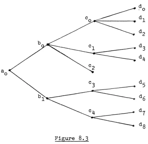
Isf> or Isl>), and the probability of getting the outcome "1" is, of course, 1 - P. Diagramatically we can represent this first measurement by the following tree with two branches.
. Temporarily decide on "0"
I-Iol-p *-Temporarily decide on "1" Figure 8.1
The transition probabilities are given by P for the branch zero, "0", and 1 - P for the branch one, 1". If the outcome
is "1", we will perform a second measurement on A characterized by the self-adJoint operator O.A Associated with 0A are the
and "0" respectively. However, if the first outcome is "O", we will perform a different measurement corresponding to O0,A' and with associated projector-valued measures 2 and I-H2
for "1" and "0" respectively. OA and 0 do not have to commute. in fact, they do not, for the optimum detection scheme (the one that minimizes the probability of error) in this example. Diagramatically we can represent both measure-ments in the following tree,
0Ott It01 -decide on "O" 1" "" decide on "1" 11 t1111
J
Figure 8.2 1 'The probabilities of the different outcome sequences are,
Pr("O","O"} = (<slHols>)(l-<alH2la>)
= <al<sl1o0 (I-12 ) s>la> (8.7)
Pr{"0 ","l" = (<slllols>)(<aflH21a>)