HAL Id: hal-01276211
https://hal.archives-ouvertes.fr/hal-01276211
Preprint submitted on 19 Feb 2016
HAL is a multi-disciplinary open access
archive for the deposit and dissemination of
sci-entific research documents, whether they are
pub-lished or not. The documents may come from
teaching and research institutions in France or
abroad, or from public or private research centers.
L’archive ouverte pluridisciplinaire HAL, est
destinée au dépôt et à la diffusion de documents
scientifiques de niveau recherche, publiés ou non,
émanant des établissements d’enseignement et de
recherche français ou étrangers, des laboratoires
publics ou privés.
Spatial instabilities in a cloud of cold atoms
Rudy Romain, Antoine Jallageas, Philippe Verkerk, Daniel Hennequin
To cite this version:
Rudy Romain, Antoine Jallageas, Philippe Verkerk, Daniel Hennequin. Spatial instabilities in a cloud
of cold atoms. 2016. �hal-01276211�
Rudy Romain,∗ Antoine Jallageas,† Philippe Verkerk, and Daniel Hennequin‡
Université Lille, CNRS, UMR 8523 - PhLAM - Physique des Lasers Atomes et Molécules, 59000 Lille, France Dense cold atomic clouds have been shown to be similar to plasmas. Previous studies showed that such clouds exhibit instabilities induced by long-range interactions. However they did not describe the spatial properties of the dynamics. In this Letter, we study experimentally the spatial nature of stochastic instabilities and find out that the dynamics is localized. Data are analyzed both in the spectral domain and in the spatial domain (principal component analysis). Both methods fail to describe the dynamics in terms of eigenmodes, showing that space and time are not separable.
PACS numbers: 37.10.Gh, 05.45.-a, 37.10.Vz, 52.35.-g
During the last decades, cold atoms have proven to be more than an extraordinary tool for studying the physics of dilute matter. Many spectacular results concern the field of condensed matter, as e.g. the direct observation of the Anderson localization [1], or that of the BEC-BCS crossover [2]. But even in the field of dilute matter, cold atoms are thought to be a good model system for plas-mas, in particular because experiments are considered to be relatively simple and well controlled. Although cold atoms in a Magneto-Optical Trap (MOT) are neutral, it has been demonstrated that a coulombian-like repul-sive force appears in the multiple scattering regime [3]. Based on this analogy, fluid-dynamical models used in plasma physics have been adapted to cold atoms physics [4–6]. On the other hand, it has been demonstrated that the dynamics of cold atoms in a MOT can be described through the Vlasov-Fokker-Planck equations [7], as e.g. the plasma dynamics in the inertial confinement fusion [8], the stellar dynamics [9] or the electron dynamics in storage rings [10].
Most of these systems are known to exhibit instabili-ties under appropriate parameter sets. Numerous types of instabilities have been observed, with very different properties and signatures. Although plasmas are gov-erned by long-range interactions, instabilities appear not only at large spatial scales, but also at smaller scales. Some examples of local instabilities are the microbunch-ing instability in the storage rmicrobunch-ings [10], drift wave mi-croinstabilities in plasmas confined by a magnetic field [11], or microinstabilities of the solar corona [12].
Instabilities in MOTs have been observed for several decades, and have been studied for 15 years. Mainly two types of instabilities have been reported through exper-iments. Self-sustained instabilities are periodic oscilla-tions [13, 14], while stochastic instabilities exhibit ran-dom characteristics [15]. In all cases, the experimental characterization is done through the temporal evolution of global variables, such as the fluorescence of the cloud or the location of its center of mass. The spatial proper-ties of the instabiliproper-ties, in particular their location in the cloud, is not known. However, most simplified models allowing to reproduce these instabilities have considered
they are global [16, 17]. On the other hand, taking for-mally into account the different processes involved in the MOTs leads to the Vlasov-Fokker-Planck equations, im-plicitly predicting local instabilities [7]. Models derived from plasmas also predict local phenomena, such as pho-ton bubbles [5], but none of them has been observed yet. Thus gaining knowledge on the spatio-temporal charac-teristics of the cloud dynamics appears to be crucial to know which methods and approximations can be used to solve the full set of equations describing the MOT. It could also help to precise the similarities between cold atoms and plasma instabilities.
We report in this paper the experimental observation of local instabilities, through a novel detection setup al-lowing to record the spatio-temporal evolution of the atoms in the MOT. We focus here on the previously ob-served stochastic instabilities [15, 16], and we show that these instabilities are localized in a limited area of the cloud. The analysis of the dynamics by two different methods does not give results consistent with the hy-pothesis of global temporal or spatial motion. The paper is organized as follows: after a brief description of the ex-perimental setup, we analyze the dynamics of the MOT through global tools, as used in the literature, in order to clearly establish the type of instabilities we are studying. Then we analyze the dynamics through two methods: the local temporal analysis gives information on the motion eigenfrequencies, while the Principal Component Analy-sis (PCA) allows to identify spatial eigenmodes.
Our experimental setup is described in detail in [14– 17]. The MOT is a standard Cs MOT with three retro-reflected beams. However, special care is taken to the stability of parameters which could introduce artefacts in the dynamics. For example, we use a single mode op-tical fiber to clean the transverse profile of laser beams. We also modulate the relative phases of all the beams to avoid possible interference patterns. The modulation frequency (> 1 kHz) is chosen larger than the collective atomic response frequencies, so that the intensity is av-eraged [18]. The MOT produces a dense cloud of cold atoms with a typical diameter of 4 mm. This size is char-acteristic of the multiple scattering regime in which the
2 collective effects play a key role in the behavior of the
cloud [19]. To obtain the desired dynamical regime, we adjust two control parameters: (i) the intensity I of a single incoming beam, expressed in units of the satura-tion intensity Isat= 1.1 mW.cm−2(D2line of133Cs) and
(ii) the detuning ∆ between the laser frequency and the atomic transition, expressed in units of the natural line width Γ = 2π × 5.22 MHz. In the following, all the il-lustrations and examples correspond to I = 11 Isat and
∆ = −1.8 Γ. They are typical of the dynamics observed for 10 Isat≤I ≤ 15 Isatand −1.9 Γ ≤ ∆ ≤ −1.6 Γ.
The spatio-temporal dynamics of the atoms is analyzed by recording the local temporal evolution of the fluores-cence at any point of the cold atom cloud. Let us re-member that the number of atoms is proportional to the fluorescence for a given set of the MOT parameters. As during an acquisition, the MOT parameters are kept con-stant, we thus record the spatio-temporal evolution of the atomic density in the cloud.
It has been shown that instabilities exhibit frequencies ranging from 1 to 100 Hz [14–17]. Thus to record the dy-namics, a standard video camera at 30 frames per second is not adapted. We use a fast video camera (Phantom v7.3 camera from Vision Research) able to record up to 10,000 frames/s. A set of lenses is used to cover an opti-cal field of 15×10 mm and a depth of field of 2.5 mm, well fitting the cloud size. An important point is to determine if the light recorded by such a camera comes only from the surface of the cloud, or from any point inside the cloud. Instabilities grow up when the atomic density is high enough, i.e. when the collective nonlinear processes inside the cloud cannot be neglected [14–17]. However, even for such relatively dense clouds, the number of scat-tering events for most photons escaping the cloud is 1 or 2 [18]. That means that the camera captures photons coming from any point inside the cloud, but with a dif-ferent weight depending on the location. This last point has to be kept in mind, although it has marginal con-sequences on the interpretation of the pictures. Indeed, the main difficulty is that we record a 2D projection of the cloud, while the dynamics occurs in 3D. This makes the interpretation of the records harder.
The location of the camera is imposed by the avail-able space on the setup. Let us call Ox, Oy and Oz the three perpendicular axes corresponding to the three in-cident beams of the trap, Oz being also the axis of the coils. The camera axis is close to the (x = y, z = 0) di-rection. Thanks to the choice of a retro-reflecting beam configuration, and because of the shadow effect [14–17], the amplitude of the dynamics is enhanced in a direction along the line x = y = 2z. The main direction of the dy-namics projects with an angle of 20° on the picture plane, leading to a satisfactory resolution of the dynamics.
In order to make the link between the present work and the previous reported observations, we also use a 4-quadrant photodiode (4QP) to monitor the total cloud
fluorescence and the position of the cloud center of mass, as e.g. in [14]. The signals from the 4QP and the pictures from the video camera are recorded synchronously.
As pointed out above, we focus here on the regime of stochastic instabilities. In [15], that regime is ana-lyzed through the dynamics of the number of atoms in the cloud and that of its center of mass. It is described to be a noisy dynamics cut off with bursts of large oscil-lations, and the analysis focused on the main frequency component, appearing inside the bursts. It is also shown that these instabilities are induced by a stochastic reso-nance centered on a given detuning.
In the present work, the unstable regime shows the same characteristics as in [12]. In particular, for the parameters given above, instabilities are maximal for ∆ = −1.8Γ; the dynamics (number of atoms and cen-ter of mass) is a succession of regular bursts and noisy intervals; in the bursts, a frequency ω1≃2π×21 Hz
dom-inates the dynamics. In order to be more exhaustive than the previous studies, we also studied the characteristics of the secondary frequency components. In the burst regime, the second component ω2 ≃ 2π × 72 Hz is two
orders of magnitude smaller than ω1. The components
2ω1and ω2−ω1are also present, with amplitudes similar
to that of ω2. In the noisy intervals, ω2 is present, with
the same amplitude as in the bursts. ω1 is also present,
but with an amplitude smaller than ω2. In summary,
ω1 appears mainly inside the bursts, while ω2 is always
present.
For this study, our aim is to characterize the nature – space dependent or not – of the dynamics. Thus we do not need to record long time series with a good time resolution, as it would be necessary for e.g. making a topological analysis of the dynamics attractors. We only need to follow the usual rules of frequency analysis, i.e. to record at least two points per period. The following results correspond to 512 × 512 pixels pictures recorded with a rate of 400 frames/s. The length of the analyzed sequences is 625 ms, i.e. 250 frames, corresponding to the typical length of the bursts.
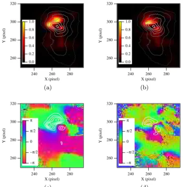
To determine the spatial dependence of the dynam-ics, a straightforward approach consists in applying the frequency analysis used previously to each point of the cloud. Fig. 1 shows a typical result for the dynamics in-side a burst. In fig. 1a, we represent in gray levels (Color online) the amplitude of the ω1component in each point
of the cloud, obtained by Fast Fourier Transform (FFT) of each pixel of the picture sequence. The dynamics ap-pears with no doubt to depend on the space. Instabilities appear in two small areas of the cloud, covering typically 10 % of the whole cloud. The two areas have very differ-ent shapes and sizes, and we see two local maxima in one of the area. Fig. 1c shows that the two areas pulse with opposite phases. It is difficult to deduce from such 2D observations the exact 3D dynamics, but it is clear that the instabilities consist in a local pulsation or rotation,
320 300 280 260 Y (pixel) 280 260 240 X (pixel) 1.0 0.8 0.6 0.4 0.2 0.0 (a) 320 300 280 260 Y (pixel) 280 260 240 X (pixel) 1.0 0.8 0.6 0.4 0.2 0.0 (b) 320 300 280 260 Y (pixel) 280 260 240 X (pixel) −π −π/2 0 π/2 π (c) 320 300 280 260 Y (pixel) 280 260 240 X (pixel) −π −π/2 0 π/2 π (d)
Figure 1: Spatial distribution of instabilities for one sequence: (a) and (b) show the local amplitude of the
two main components: ω1and ω2. The normalized
magnitude squared of the spectral component is represented in gray level (Color online). The contour
plot shows the averaged fluorescence during the sequence. (c) and (d) represent the corresponding phase
distributions. Grayscale (Color online) represents the relative phase of the local oscillation between ±π. The
contour plot identifies the unstable areas.
while the rest of the cloud is stable.
The above example is typical of what we observed in all recorded sequences. Some differences appear, as the location of the unstable area, its structure, in particular the number of local maxima, and its shape, but we always observed that the instabilities were localized in a limited area of the cloud, covering typically 10 % of the whole cloud.
We performed the same analysis for the ω2component,
and found the same type of results as for the ω1
compo-nent: the instabilities are localized in a relatively small area, and they correspond to a motion of pulsation or ro-tation of a part of the cloud. As discussed above, inside the bursts, the ω2component is small as compared to the
ω1 component, making the analysis of data less reliable.
However, it appears clearly that in this case, the char-acteristics of the ω2 component follow those of the ω1
component, delimiting the same unstable area with the same type of motion. Figs 1b and 1d show respectively the amplitude and the phase of the ω2 component for
the same burst as figs 1a and 1c: the spatial distribution
of the instabilities are the same for the two components. The similarity of the phase distributions is less convinc-ing, due to the weakness of the component, but in spite of that, a phase opposition appears between the two areas. To generalize this observation, we computed the spatial overlap between the two components for all the recorded sequences, and found that they have in most cases a sim-ilar spatial distribution.
Outside the bursts, the ω2 component is still present,
and has the same characteristics. Thus the dynamics ap-pears to be a small (in space) and weak (in amplitude) periodic motion of a small part of the cloud at the ω2
frequency, cut off by bursts where the amplitude of the motion increases temporarily, while its main frequency shifts to ω1. However, this description is not completely
satisfactory. Indeed, it gives information about the tem-poral components of the dynamics, but does not give any information about the spatial components. In par-ticular, it seems to associate one spatial component with two different frequencies, while in spatio-temporal sys-tems where the temporal dynamics and the space distri-bution can be separated, as e.g. in multimode lasers [20], a spatial eigenmode is associated with only one eigenfre-quency. We adopt in the following another approach.
PCA presents the advantage to give a description of the dynamics of the system without requiring any prelim-inary hypothesis. The dynamics is described in terms of a superposition of spatial modes, giving complementary information with respect to the Fourier analysis. The analysis is performed using the method described in [21]. The result of the PCA is a set of spatial modes forming a basis whose size is equal to the number of pictures of the sequence (250 in our case). If these modes are sorted ac-cording to their weight, i.e. their contribution to the to-tal statistical deviation around the averaged atomic dis-tribution, the method leads to the determination of the number of modes useful to describe the dynamics. In our case, we find that in the sequences considered here, the main mode contains between 50 % and 80 % of the statis-tical fluctuations, and the second mode between 5 % and 25 %. Thus the dynamics appears to be dominated by one single mode, although the weight of the second mode is not negligible. Depending on the desired accuracy, the third mode, with a weight of 10 % ± 5 %, could be taken into account. In the following, we consider only the first two modes.
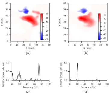
Figure 2 shows the first two modes obtained by the PCA of the sequence of figure 1. Note the similarity of the main mode with the ω1spatial distribution (fig. 1a).
However, this result is not general. On the contrary, we observe a major difference between the modes given by the PCA and the ones resulting from the Fourier analysis. While in the latter a wide variety of shapes are obtained, the results are more homogeneous in the former. In fact, one set of modes dominates the whole dynamics. This basis – let us call it the main basis – is not the only one
4 60 50 40 30 20 10 0 Y (pixel) 60 50 40 30 20 10 0 X (pixel) -60 -40 -20 0 20 40 60 (a) 60 50 40 30 20 10 0 Y (pixel) 60 50 40 30 20 10 0 X (pixel) -80 -60 -40 -20 0 20 40 60 80 (b)
Figure 2: Two first spatial modes given by the PCA (2a and 2b respectively) for the same sequence than in
figure 1. In both cases, the spatial distribution is represented in absolute value in gray level (Color online), and the upper and the lower areas have to be
understood respectively as an excess (in blue online) and a depletion of atoms (in red online). This information is similar than the one given by the phase
of the Fourier analysis.
found by the PCA, but it is the most frequent in the set of recorded sequences. This regime is randomly interrupted by short intervals where the dynamics is described by another basis, before it returns to the main basis. These alternative bases differ from one sequence to another one, and we did not found any common properties. For exam-ple, in a few cases, the modes of the main basis appear, but in a different order: the first mode of the main basis becomes the second mode of the basis.
A surprising result is that the regimes found with the PCA do not correspond to those given by the Fourier analysis. In particular, the sequences described by the main basis do not follow the succession of bursts and noisy intervals. As a consequence, the frequencies associ-ated with the main basis may change from one sequence to another. Moreover, the time evolution of a given spa-tial mode may exhibit different frequencies in different sequences. Fig. 3 shows the time evolution and the FFT of two modes dominating the dynamics in two consecu-tive sequences. Although the two modes are similar, they are associated with two very different time evolution: for the first one, both frequencies ω1and ω2drive the
dynam-ics, while the second one corresponds to a burst where ω1 dominates the dynamics.
In summary, the PCA leads to a description of the dy-namics in terms of spatial modes. The results show that such a description is as relevant as the description in terms of frequency components. Two regimes are found: the first one corresponds to a well identified spatial mode basis, referred as the main basis, and a second one, de-scribed by different bases. From this point of view, the description obtained by the PCA is similar to that of the Fourier analysis. But surprisingly, the two regimes
60 50 40 30 20 10 0 Y (pixel) 60 50 40 30 20 10 0 X (pixel) -60 -40 -20 0 20 40 60 (a) 60 50 40 30 20 10 0 Y (pixel) 60 50 40 30 20 10 0 X (pixel) -60 -40 -20 0 20 40 60 (b) 1.0 0.5 0.0
Spectral power (arb. unit) 0 20 Frequency (Hz)40 60 80 100
(c)
1.0
0.5
0.0
Spectral power (arb. unit) 0 20 Frequency (Hz)40 60 80 100
(d)
Figure 3: From top to bottom: first modes calculated by the PCA for two consecutive sequences and the FFT
of the time evolution of these modes.
of the PCA do not correspond in time sequences to the two regimes of the Fourier analysis. Thus the two ap-proaches – temporal and spatial – give complementary information on the dynamics: the dynamics of the cloud of cold atoms in a MOT is a genuine spatio-temporal sys-tem, where the spatial and temporal behaviors cannot be separated.
We report in the present paper experimental results on the dynamics of an unstable cloud of cold atoms in a regime of stochastic instabilities. Previous studies fo-cused on the temporal behavior of the instabilities. Here we study both the spatial and temporal properties of the dynamics. Although the atomic motion cannot be clearly identified as our analysis is based on a 2D projection of a 3D motion, we show that the oscillations are localized in space. We analyze the dynamics through two differ-ent methods, and both point out the key role of space in the dynamics. Moreover, the analyses in terms of fre-quency components and in terms of spatial modes show that the relation between the temporal regime and the spatial distribution is not straightforward, as the same spatial distribution can correspond to different tempo-ral regimes. These results invalidate the description in terms of purely temporal models, as in [13–17], and re-quire the use of fully spatio-temporal models, as the Vlasov-Fokker-Planck model [7] or plasma-derived model [5]. They strengthen the relationship between cold atoms and plasmas, and show that cold atoms could be a good model system for plasmas. However, a fine comparison of both systems and a deep physical interpretation of the observed behavior require a better knowledge of the dy-namics of cold atoms. So, the next step is to run
numeri-cal simulations to obtain quantitative agreement between models and experimental observations, in particular in the dynamical regimes.
ACKNOWLEDGMENTS
The authors would like to thank R. Dubessy for helpful discussions about the PCA. This work was supported by the Labex CEMPI (Grant No. ANR-11-LABX-0007-01) and “Fonds Européen de Développement Economique Régional”.
∗ Current address: Department of Physical Sciences, The Open University, Walton Hall, MK7 6AA, Milton Keynes, United Kingdom
† Current address: Laboratoire Temps-Fréquence, Institut de Physique, Université de Neuchâtel, Avenue de Belle-vaux 51, 2000 Neuchâtel, Switzerland
‡ Corresponding author: [email protected]; Permanent address: Laboratoire PhLAM Bât. P5 - Uni-versité Lille, 59655 Villeneuve d’Ascq cedex, France [1] F. Jendrzejewski, A. Bernard, K. Müller, P. Cheinet, V.
Josse, M. Piraud, L. Pezzé, L. Sanchez-Palencia, A. As-pect and P. Bouyer, Nature Physics 8, 398 (2012) [2] T. Bourdel, L. Khaykovich, J. Cubizolles, J. Zhang, F.
Chevy, M. Teichmann, L. Tarruell, S. J. J. M. F. Kokkel-mans, and C. Salomon, Phys. Rev. Lett. 93, 050401 (2004)
[3] L. Pruvost, I. Serre, H. T. Duong, and J. Jortner, Phys. Rev. A 61, 053408 (2000)
[4] J. T. Mendonça, R. Kaiser, H. Terças and J. Loureiro, Phys. Rev. A 78, 013408 (2008)
[5] J. T. Mendonça and R. Kaiser, Phys. Rev. Lett 108, 033001 (2012)
[6] J. D. Rodrigues, J. A. Rodrigues, A. V. Ferreira, J. T. Mendonça, Opt. Quant. Electron. 48, 169 (2016) [7] R. Romain, D. Hennequin, and P. Verkerk, Eur. Phys. J.
D 61, 171 (2011)
[8] C. P. Ridgers, R. J. Kingham, and A. G. R. Thomas, Phys. Rev. Lett. 100, 075003 (2008)
[9] Pierre-Henri Chavanis, Phys. Rev. E 68, 036108 (2003) [10] E. Roussel, C. Evain, C. Szwaj, and S. Bielawski, Phys.
Rev. ST Accel. Beams 17, 010701 (2014)
[11] Jan Weiland, Stability and Transport in Magnetic Con-finement Systems, Springer Series on Atomic, Optical and Plasma Physics 71 (Springer, New-York, 2012) [12] Eckart Marsch, Living Rev. Solar Phys. 3, 1 (2006) [13] G. Labeyrie, F. Michaud, and R. Kaiser, Phys. Rev. Lett.
96, 023003 (2006)
[14] Andrea di Stefano, Marie Fauquembergue, Philippe Verkerk, Daniel Hennequin, Phys. Rev. A 67 033404 (2003)
[15] David Wilkowski, Jean Ringot, Daniel Hennequin, Jean Claude Garreau, Phys. Rev. Lett. 85 1839 (2000) [16] D. Hennequin, Eur. Phys. J. D 28 13 (2004)
[17] A. di Stefano, Ph. Verkerk, D. Hennequin, Eur. Phys. J. D 30 243 (2004)
[18] R. Romain, H. Louis, P. Verkerk and D. Hennequin, Phys. Rev. A 89, 053425 (2014)
[19] D.W. Sesko, T.G. Walker, and C. Wieman, J. Opt. Soc. Am. B 8 946 (1991)
[20] D. Hennequin, D. Dangoisse, P. Glorieux, Opt. Commun. 79200–206 (1990)
[21] R. Dubessy, C. De Rossi, T. Badr, L. Longchambon and H. Perrin, New J. Phys. 16 122001 (2014)