Publisher’s version / Version de l'éditeur:
Proceedings 9th International Offshore and Polar Engineering Conference
ISOPE'99, 2, pp. 659-664, 1999-05
READ THESE TERMS AND CONDITIONS CAREFULLY BEFORE USING THIS WEBSITE.
https://nrc-publications.canada.ca/eng/copyright
Vous avez des questions? Nous pouvons vous aider. Pour communiquer directement avec un auteur, consultez la
première page de la revue dans laquelle son article a été publié afin de trouver ses coordonnées. Si vous n’arrivez pas à les repérer, communiquez avec nous à [email protected].
Questions? Contact the NRC Publications Archive team at
[email protected]. If you wish to email the authors directly, please see the first page of the publication for their contact information.
NRC Publications Archive
Archives des publications du CNRC
This publication could be one of several versions: author’s original, accepted manuscript or the publisher’s version. / La version de cette publication peut être l’une des suivantes : la version prépublication de l’auteur, la version acceptée du manuscrit ou la version de l’éditeur.
Access and use of this website and the material on it are subject to the Terms and Conditions set forth at
Adapting the Canadian Ice Regime System to operational ice navigation
Frederking, R.
https://publications-cnrc.canada.ca/fra/droits
L’accès à ce site Web et l’utilisation de son contenu sont assujettis aux conditions présentées dans le site LISEZ CES CONDITIONS ATTENTIVEMENT AVANT D’UTILISER CE SITE WEB.
NRC Publications Record / Notice d'Archives des publications de CNRC:
https://nrc-publications.canada.ca/eng/view/object/?id=3ba2c30f-e5ac-47f1-818f-852bb9def72f
https://publications-cnrc.canada.ca/fra/voir/objet/?id=3ba2c30f-e5ac-47f1-818f-852bb9def72f
Proceedings of the Ninth (1999) International Offshore and Polar Engineering Conference Volume II, pp 659-664,
Brest, France, May 30-June 4, 1999
Adapting the Canadian Ice Regime System to Operational Ice Navigation
R. Frederking
National Research Council of Canada Ottawa, Canada
Abstract
The Canadian Arctic Ice Regime Shipping System (AIRSS) uses ice conditions and vessel class to provide guidance on safe navigation in ice. In this paper the AIRSS has been modified to take into account ice decay, ridging, floe size and icebreaker escort to calculate a Transit Numeral, an indicator of ice severity. Transit Numerals have been determined for a number of vessels operating in the Russian Arctic and in turn related to average vessel speed. The ice navigation data have been analysed to predict mean speed, standard deviation of speed and an upper limit average transit speed. These transit speeds provide an experience-based indication of expected long-term ship performance in actual practice along the Northern Sea Route.
Key Words: Ice navigation, ice conditions 1. Introduction
Commercial shipping in the Arctic must be both safe and economical. Traditionally such navigation has been based on the skill of the Captain and crew, and a vessel adequate for the ice conditions. With the envisioned expansion of international marine traffic through various Arctic sea routes it is not expected that the same level of operational skill will be available on all transiting vessels. Training will be one important factor in providing the required skills; however, other aids to safe and economic navigation will also be required.
There are already systems in place in several countries to assist navigation in ice. In Canada the Arctic Ice Regime Shipping System (AIRSS) (Transport Canada, 1996) has been implemented as part of a revised Arctic Shipping Pollution Prevention Regulations (ASPPR, 1989). ASPPR is oriented to safety of shipping operations, setting requirements for hull strength, machinery strength and the limiting ice conditions in which various categories of vessels are permitted to operate. The AIRSS provides advice on whether a particular class of vessel can advance into an area having a specific set of ice conditions. In Russia, the Russian Registry maintains a classification of icebreakers and icebreaking vessels. There is additionally an Ice Passport (Likhomanov et al, 1998) that provides guidance to the captain on safe speed for navigation in various ice conditions, and a
QAD (Quantitative Assessment of navigation Difficulty in ice) system (Brovin et, 1995) which provides a quantitative means for predicting transit speeds.
In the present work, the Canadian AIRSS is modified to make it more suitable for planning and managing vessel transit. The AIRSS does not take into account ship operations (vessel speed, visibility, etc.) in a direct fashion. It does, however, take advantage of current ice condition information generated by most national ice services, supplemented by detailed ice observations available on-board the vessel to guide safe transit. The same ice information, in a recast form, can provide a useful guide for the maximum speed with which a vessel may proceed through ice. Information on Russian navigation experience in the Arctic will be used to develop an experience-based model. This model can be used to predict transit times for particular classes of vessels in relation to quantifiable ice conditions (average and extreme) for particular regions and seasons. It can also be used to select a preferred routing. This paper will briefly describe the AIRSS and how it has been modified to make it suitable for providing guidance on route selection based on actual ice conditions as determined from normal ice charts.
2. Description of Canadian Arctic Ice Regime Shipping System
The AIRSS was developed to provide guidance on safety of navigation in the Canadian Arctic. It relates the level of hull strength of a vessel to the actual ice conditions through which the vessel will transit. Based on this assessment of ice conditions in relation to ship type or class, the vessel is either allowed to proceed to not. AIRSS is strictly safety oriented; there is no provision for special operations, i.e. lower speed, extra caution, etc., which would allow a vessel to proceed into an otherwise forbidden ice condition. Similarly, it provides no operational guidance on how a vessel is allowed to proceed, other than due caution of mariners.
The core of AIRSS is the quantitative description of ice conditions. The starting point is an ice regime, that is, a geographic area composed of a relatively uniform distribution of any mix of ice types, including open water. Thus an ice regime can have dimensions of several 10s of m to several 10s of km. The World Meteorological Organization (WMO) nomenclature is used to describe the ice types. Shorthand for this is the WMO Ice Code or “egg” code. The code provides
information on partial ice concentration, Ci, stage of development
(thickness), Si, and predominant floe size for each partial concentration,
Fi. Usually only the three oldest (thickest) ice types are included, but
this can be extended as necessary.
In the Canadian regulations (ASPPR, 1989), the ship’s structure must be designed to safely withstand impacts with a maximum thickness of ice. This is the thickest ice type in which a properly navigated ship may operate without risk of structural damage. The regulations define 9 categories of vessels such that each ship category is related to a specific ice type (thickness). The vessel category, and ice capability, increases with increasing ice thickness.
An ice regime has two components: 1) ice that is thicker (or more severe than) the ice specified for the vessel; and 2) ice thinner than that specified. These two components always total 10/10ths. In any given ice conditions, the ratio of the two components will differ between ship categories, since each ship category has a different specific ice. The risk of damage, therefore, will depend on the proportions of hazardous ice (i.e. ice thicker than that specified for the vessel) and non-hazardous ice (thinner ice) in the regime.
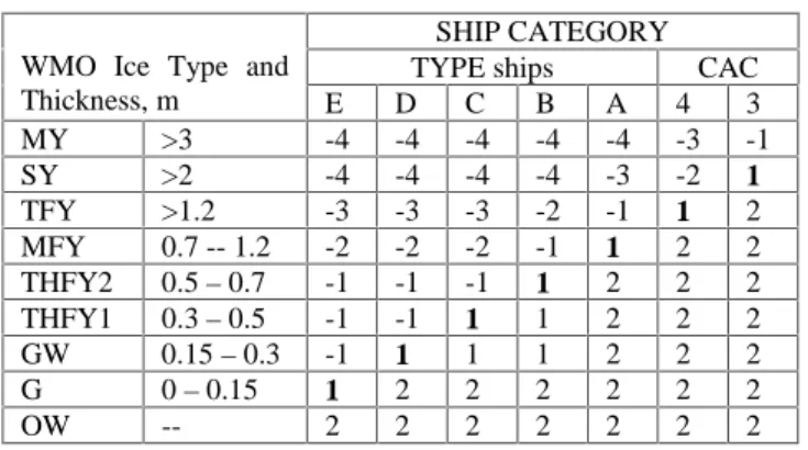
To quantify the ice regime, a scheme has been developed which takes into account the relative amount of each type of ice, and relates it to the ship category. This is reflected through an Ice Multiplier (IM). The value of the Ice Multiplier reflects the level of danger that the particular ice type poses to the particular category of ship, with the larger negative numbers representing larger hazards. For more explanation of Ice Multipliers WMO ice types and ship categories, see Transport Canada (1996). Table 1 lists the Ice Multiplier values for each ship category). The specified ice for that category of ship is shown in bold.
Table 1 Ice Multipliers for each Ship Category
SHIP CATEGORY
TYPE ships CAC
WMO Ice Type and
Thickness, m E D C B A 4 3 MY >3 -4 -4 -4 -4 -4 -3 -1 SY >2 -4 -4 -4 -4 -3 -2 1 TFY >1.2 -3 -3 -3 -2 -1 1 2 MFY 0.7 -- 1.2 -2 -2 -2 -1 1 2 2 THFY2 0.5 – 0.7 -1 -1 -1 1 2 2 2 THFY1 0.3 – 0.5 -1 -1 1 1 2 2 2 GW 0.15 – 0.3 -1 1 1 1 2 2 2 G 0 – 0.15 1 2 2 2 2 2 2 OW -- 2 2 2 2 2 2 2
For any ice regime, an Ice Numeral (IN) is calculated by taking the sum of the products of the concentrations of the ice types present (in 10ths), and their ice multiplier. The Ice Numeral is defined as:
IN = (Ca x IMa) + (Cb x IMb) + ... (1)
where IN is the Ice Numeral, Cn is the concentration (in tenths) of ice
type “n”, and IMn is the Ice Multiplier from Table 1. The right side of
the equation is expanded to include all the types of ice that are present, including open water. Note that the total of the partial concentrations (ice and open water) must add up to 10 tenths. The Ice Multipliers (IM) may be either positive or negative, depending on the ice type and ship category, so when combined into an Ice Numeral (IN) they represent a quantitative measure (a weighted average) of the ice regime in relation to a ship’s structure. The Ice Numeral therefore depends on the particular ice regime and category of ship operating within its boundaries. The system takes into account ice decay and ice ridging.
For any given ship category, entry or non-entry into an ice regime is determined by the sign of the Ice Numeral. If the IN is negative, entry is not allowed. However, if the IN is zero or positive, then entry by the ship into that ice regime is allowed. The system does not make any allowance for the magnitude of the Ice Numeral. The Ice Multipliers in Table 1 are empirically based. They were initially established from judgement and experience of many Canadian Arctic mariners. Subsequently a number of validation voyages were conducted to adjust the multipliers and establish the effects of ice decay and ridging. Currently there is a project underway to put the AIRSS on a more scientific basis (Timco et al, 1997).
3. Russian Ice Navigation Data
Analysed data of Russian ice navigation experience for a number of vessels were procured from the Arctic and Antarctic Research Institute (Timofeev et al, 1997) as part of a study being conducted for Transport Canada on validating the Canadian Arctic Ice Regime Shipping System. The vessels studied were part of the fleet of the Murmansk Shipping Company. The experience, from the first half of the 1980s, covered both successful navigation in ice and a very small number of damage events.
The data were divided into two groups: the first examined the experience of the "Ivan Susanin", a Russian Registry type UL vessel for four ice navigation seasons from 1981 to 1985; and the second examined 3 types of ships, ULA, UL and Ll for a single season (1983-84). L1, UL and ULA are Russian Registry designations for progressively more ice able vessels. Information on the ship particulars is summarized in Table 2. More details on the ships can be found in Timofeev et al (1997).
Table 2 Description of Ships
Ice Class of Ships ULA UL L1
Name of Ship Series “Norilsk” “Dmitry Donskoy” “Pioner” Length overall (m) 174.0 162.1 105.7 Breadth (m) 24.5 22.86 15.6 Summer Draft (m) 10.5 9.88 6.8 Deadweight (t) 20,000/14,700 19,885 4648 Service Speed (kn) 17.0 15.2 13.8 Power (kW) 13,850 8240 2390
For the Ivan Susanin there were 136 voyage segments and for the 1983-84 season there were 555 voyage segments involving 24 different ships. Date, time, name of geographic location and coordinates of start and end points of each segment were given, so average transit speeds could be determined for each voyage segment. Average ice conditions, according to WMO nomenclature, were give for each voyage segment. This allows vessel progress to be related to ice conditions. Detailed results of this analysis are given in Frederking (1998).
The area covered by this navigation experience was the Russian Arctic, primarily from Murmansk as far east as Dikson, but there were a few voyages across the entire Northern Sea Route. Navigation from Murmansk to Dudinka is conducted on a year round basis and includes transits through the Pechora Sea, Kara Sea and Yenisey River.
4. Modification of AIRSS for Operational Application
As was pointed out previously, the Canadian Arctic Ice Regime Shipping System relates ice conditions to ship capability and advises on entry into an ice regime. This is done through a quantification of the ice regime using the WMO egg code and a system of Ice
Multipliers to calculate an Ice Numeral that determines whether the ship should advance into that ice regime. In adapting the AIRSS for operations it has been decided to start from the same basis of the WMO ice code to quantify the ice conditions. However, different ice multipliers have to be established to allow the ice information to be used for operations. As a starting point for setting ice multipliers, the following assumptions will be made
- ice multipliers will always be taken to be positive - ice multiplier for open water will be the same for all
classes or types of ships
- the minimum ice multiplier for the most severe ice for each class or type of ship will be zero
- the most severe ice for each class or type of ship will increase in thickness as the ice capability of the vessel increases
- the ice multiplier will vary with ice thickness
- regardless of the ship class, the same magnitude of ice numeral should reflect a similar level of risk and difficulty for that speed
In addition to the ice multipliers discussed above, adjustment for ice decay, ridging and floe size will be applied. Decay is accounted for by adding 1 to each of the ice multipliers for medium and thick first year sea ice, and second year and multi-year ice. In this study it is assumed that during the months of June through September ice is decayed. Ridging is accounted for by subtracting 1 from the multiplier of each ice type for which the proportion of ridging is 2 fifths or more, and provided the total ice concentration is greater than 6 tenths. The influence of floe size is taken into account by adding 1 to each ice type for which the floe size is 20 m or less, that is WMO floe size codes 1 or 2. The effect of an icebreaker breaking a channel is accounted for by considering the floe size in the broken channel to be less than 20 m. The result of this operation is the determination of a Transit Numeral,
TN, which is defined by the following equation
TN = (Ca x (TMa + D – R + F)) + (Cb x (TMb + D – R + F)) + ...(2)
where , Cn is the concentration (in tenths) of ice type “n”, TMn is the
Transit Multiplier for that ice type and ship category, D is the adjustment for decay, R is the adjustment for ridging, and F is the adjustment for floe size. A higher Transit Numeral would be expected to be associated with a higher speed, and a lower Transit Numeral with a lower speed. A set of Ice Multipliers has been established for the three classes of Russian Registry ships for which ice transit data are available. The multipliers are given in Table 3 below.
Table 3 Transit Multipliers for determination of Transit Numeral for Russian Registry ships
Ice Type and Thickness, m L1 UL UL A >3 -- -- 0 >2 -- -- 2.0 >1.2 -- 0 3.6 0.7 -- 1.2 0 2.3 4.2 0.3 – 0.7 3.2 4.0 4.7 0.15 – 0.3 4.4 4.7 4.9 0.1 – 0.15 5 5 5 0 – 0.1 5 5 5 MY SY TFY MFY THFY GW G New OW -- 5 5 5
The multipliers range from 5 for open water to 0 for ice in which it is expected a ship of that type would just be able to move continuously under full power. The decrease in ice multiplier with increasing ice
thickness is taken to be proportional to ice resistance. Ice resistance is assumed proportional to ice thickness raised to the 1.5 power. All the ice information to calculate a Transit Numeral can be obtained from an ice chart on which ice regimes are designated with a WMO egg code. The application of these multipliers for a particular ice regime will result in a Transit Numeral for a particular type of ship. For a given Transit Numeral, it is proposed that there is an average transit speed which, if exceeded, would result in an elevated risk of damage. Additionally there is a range of speeds that represent what ships actually realize in practice. In the following two sections, the empirical approach using Transit Multipliers to determine Transit Numerals will be tested against navigation data from the Russian Arctic.
5. Application of AIRSS to Ivan Susanin data for several seasons
The four seasons of ice navigation experience with the Ivan Susanin provide a number of opportunities for analysis of the results. The Ivan Susanin is classified as UL under the Russian Registry of ships. The navigation experience of the Susanin will be examined in terms of expected transit speed using the modified AIRSS.
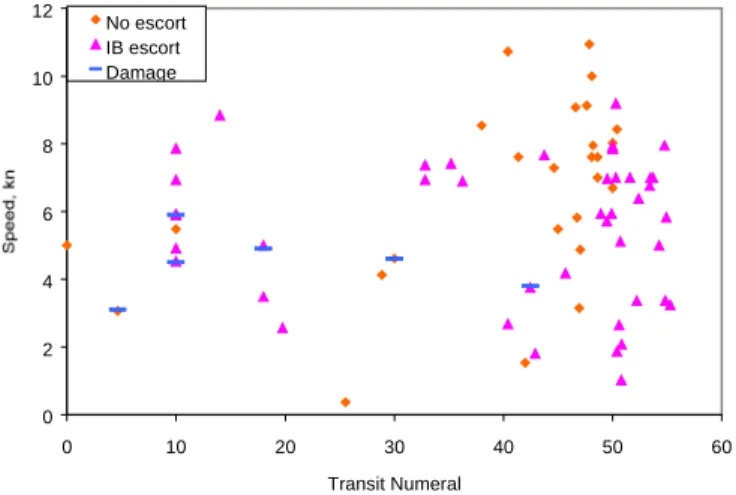
Using the methodology described in Section 4, Transit Numerals were calculated for the Susanin navigation experience. The results presented in Figure 1 show the average speed in knots in relation to the calculated Transit Numeral. The Transit Numerals include the effects of decay, ridging and floe size. The influence of icebreaker escort is taken into account by assuming that the icebreaker reduces the floe size to the range 2 to 20 m, WMO floe size category 2. Referring to Figure 1, it can be seen that there is no clear trend of speed as a function of Transit Numeral. A simple analysis of all the data indicates a mean transit speed of 6 kn with a standard deviation of 2.5 kn. Transit speed of voyage segments with icebreaker escort seems to be particularly independent of Transit Numeral. In Figure 2 the data are plotted again with the icebreaker escorted segments removed. Now there is a much clearer trend of decreasing transit speed with decreasing Transit Numeral. 0 2 4 6 8 10 12 0 10 20 30 40 50 60 Transit Numeral No escort IB escort Damage
Figure 1 Transit speed of the Ivan Susanin as a function of Transit Numeral for years 1981-85
Another approach to the analysis is to examine transit speed as a function of month of the year in which that voyage segment commenced, see Figure 3. Note that only the data for unescorted voyages are considered. There is scatter in the data, but it can be seen that there is a general trend of decreasing speed from January through to May, and then a trend of constant speed from July through December.
0 2 4 6 8 10 12 0 10 20 30 40 50 60 TRANSIT NUMERAL
Figure 2 Transit speed of the Ivan Susanin for the years 1981/85 as a function of the Transit Numeral, escorted voyage segments removed 0 2 4 6 8 10 12 1 2 3 4 5 6 7 8 9 10 11 12 Month of Year
Figure 3 Seasonal variation of Transit Speed for Ivan Susanin, escorted voyage segments removed
6. Application to different vessels in one season
For the 1983/84 shipping season, data from over 700 voyage segments for three Russian Registry classes were available for analysis. These voyage segments cover a large part of the Russian Arctic, with some voyages traversing the entire Northern Sea Route. As discussed before, there are no direct equivalencies between the Russian Registry classes and ASPPR, however as a starting point ULA was treated as CAC4, UL as Type A and L1 as Type B. The ice navigation experience or these three classes will each be examined in turn.
6.1 ULA Vessels
Transit Numerals were calculated for the ULA vessels using the Transit Multipliers from Table 3. The resulting of average transit speeds versus Transit Numerals are plotted in Figure 4. It is possible to estimate an upper envelope curve of maximum anticipated average transit speed as a function of Transit Numeral. Transit speed is taken to increase uniformly with Transit Numeral up to 13 kn at a TN of 40 and then remain constant. For Transit Numerals between 35 and 55 the mean transit speed is 8 kn with a standard deviation of 2 kn. Thus the
upper envelope speed is equivalent to the mean plus 2 ½ standard deviations. Note that these data include voyages to Dudinka as well as 4 voyages across the Northern Sea Route. For comparison the voyages across the Northern Sea Route have been separated out and plotted in Figure 5. For the Northern Sea Route section the mean transit speed is 7.5 kn, a slight decrease from the overall mean.
0 5 10 15 0 10 20 30 40 50 60 Transit Numeral
Figure 4 Transit Numerals as a function of transit speed for ULA vessels 0 5 10 15 0 10 20 30 40 50 60 Transit Numeral
Figure 5 Transit Numerals as a function of transit speed for ULA vessels on Northern Sea Route
6.2 UL Vessels
Transit Numerals for the UL vessels were calculated using the Transit Multipliers from Table 3. The results of transit speed versus Transit Numeral are plotted in Figure 6. These results are similar to Figure 1 for the Susanin, which is also a UL vessel. No clear trend of decreasing transit velocity with decreasing Transit Numeral is apparent. For Transit Numerals from 35 to 55 mean transit speed is 9 kn with a standard deviation of 2.5 kn. This speed is higher than the value of 6 kn for the “Ivan Susanin” over the period 1981 to 1985. For a closer comparison, Susanin data for 1983/84 was examined; however the mean transit speed for this period was 6.5 kn.
0 5 10 15 0 10 20 30 40 50 60 Transit Numeral
Figure 6 Transit Numerals as a function of speed for UL vessels
6.3 L1 Vessels
Transit Numerals for the L1 vessels were calculated using the Transit Multipliers from Table 3. The results of transit speed versus Transit Numeral are plotted in Figure 7. In this case a trend of increasing transit velocity with increasing Transit Numeral is apparent. For Transit Numerals from 35 to 50 mean transit speed is 7.2 kn with a standard deviation of 3.4 kn. The trend line indicated in this figure increases linearly to 10.6 kn (mean speed plus one standard deviation) at a Transit Numeral of 40, and then remains constant. This trend line represents an upper limit of likely average transit speed for an L1 vessel in the ice conditions described by the Transit Numerals.
0 5 10 15 0 10 20 30 40 50 60 Transit Numeral
Figure 7 Transit Numerals as a function of speed for L1 vessels 7. Discussion
Ice conditions, ship capability and operational skill are the three factors which combine to provide for safe and economical navigation in ice. The analysis and prediction of ship capability in the sense of structural strength and powering is perhaps the most technically advanced of the three factors. The quantification of ice conditions and their relation to ship safety and performance is still an area of active research. Ice conditions vary both spatially and temporally. While quantifiable in one respect (thickness, strength, floe size, ridging, etc.), they are difficult to quantify in a manner, which relates them to ice navigation
performance. Currently there is a comprehensive research project underway on defining “ice state” (Tuhkuri et al, 1997). The future will undoubtedly bring improved characterizations of ice conditions. Finally, operational skill is the least quantified factor and yet the most important.
The modification of the AIRSS to generate Transit Numerals as an indicator of average transit speed produced mean and upper limit average transit speeds that could be realized in actual practice in the Russian Arctic. It had been anticipated that there would be a more definitive relation between average transit speed and Transit Numeral. While not presented in the report, numerous variations of Transit Multipliers and corrections for decay, ridging and floe size were tried, however none produced clearer results. It appears that uncertainty in defining the ice conditions and actual transit speeds in ice preclude trying to refine the analysis any further at this time. In certain cases it is known that vessels stopped, perhaps to wait for icebreaker escort or for other reasons, resulting in low average transit speeds. There is no way at this time to filter out questionable average speeds. The average transit speed results should be treated as “operating gross ice velocity” as defined by Brovin et al (1995). As such they are a true indication of transit speed which are likely to be realized in actual operations. In the case of ULA and L1 vessels a speed dependency on Transit Numeral could be set. What can be drawn from the transit speed analysis is a value of mean and standard deviation of transit speed for various vessels. This is presented in Table 4.
Table 4 Mean and standard deviation of transit speed
Vessel Season/Area Mean Speed Standard Deviation Number of Samples kn kn Ivan Susanin All seasons 5.9 2.4 70 “ 1981-82 5.9 3.2 20 “ 1982-83 4.8 2.6 12 “ 1983-84 6.5 1.7 17 ‘ 1984-85 6.7 1.7 11 ULA 83-84/overall 8.0 2.1 197 “ 83-81/NSR 7.6 2.6 39 UL 83-84 9.3 2.5 93 L1 83-84 7.2 3.4 17
These values can generally be used to predict expected average transit speed provided ice conditions are characterized by a Transit Numeral greater than about 35 as calculated with the Transit Multipliers given in Table 3.
8. Conclusions
- Modification of the AIRSS to generate Transit Numerals provides a means for predicting average transit speeds which particular classes of vessels will realize under actual operating conditions along the Northern Sea Route provided the Transit Numeral is greater than 35. - Data quality do not permit any further refinement of a
proportional dependence of transit speed on magnitude of the Transit Numeral.
- WMO egg code definition of ice conditions, in the absence of any other accepted means, is the best method for classifying ice regimes from the perspective of safety and efficacy of ice navigation.
9. Acknowledgements
This project was supported by the International Northern Sea Route Project. The interest and support of Victor Santos-Pedro at Transport Canada in this work is acknowledged, as well as the assistance of Jelte Borneman, a work term student at Transport Canada.
10. References
ASPPR, 1989, Proposals for the Revision of the Arctic Shipping Pollution Prevention Regulations, Transport Canada, December 1989, Transport Canada Publication No. TP 9981.
Brovin, A. and Tsoy, L., 1995, Planning and Risk Assessment, Volume 1 – 1993 project work, INSROP Working Paper No. 23 – 1995, I.5.5.
Frederking, R. 1998, Modification of the Canadian Ice Regime System to Include Ship Operations, INSROP Working Paper in press. Likhomanov, V., Timofeev, O., Stepanov, I. and Kashtelyan, V., 1998,
Ice Passport for Icebreaker “Pierre Radisson” and Passport’s concept: Further Development, Proc. 8th (1988) International Offshore and Polar Engineering Conference, Montreal, May 24-29, 1998, Vol. II, pp. 566-571.
Timco, G.W., Frederking, R. and Santos-Pedro, V., 1997, A Methodology for Developing a Scientific Basis for the Ice Regime System, Proc. 7th (1987) International Offshore and Polar Engineering Conference, Honolulu, May 25-30, 1997, Vol. II, pp. 498-503.
Timofeev, O., Frolov, S. and Klenov, A., 1997, Compilation and Analysis of Russian Navigation Experience, Report of Arctic and Antarctic Research Institute, St. Petersburg, October 1997, Transport Canada Publication No. TP 13159.
Transport Canada, 1996, Arctic Ice Regime Shipping System (AIRSS) Standards, Transport Canada, June 1996, Transport Canada Publication No. TP 12259.