Monitoring the thermal performance of the above-grade portion of basement walls with exterior insulation

Publisher’s version / Version de l'éditeur:

Vous avez des questions? Nous pouvons vous aider. Pour communiquer directement avec un auteur, consultez la Questions? Contact the NRC Publications Archive team at

PublicationsArchive-ArchivesPublications@nrc-cnrc.gc.ca. If you wish to email the authors directly, please see the first page of the publication for their contact information.

https://publications-cnrc.canada.ca/fra/droits

L’accès à ce site Web et l’utilisation de son contenu sont assujettis aux conditions présentées dans le site LISEZ CES CONDITIONS ATTENTIVEMENT AVANT D’UTILISER CE SITE WEB.

Internal Report (National Research Council of Canada. Institute for Research in Construction), 2000-09-14

READ THESE TERMS AND CONDITIONS CAREFULLY BEFORE USING THIS WEBSITE.

https://nrc-publications.canada.ca/eng/copyright

NRC Publications Archive Record / Notice des Archives des publications du CNRC :

https://nrc-publications.canada.ca/eng/view/object/?id=f8125bd7-a681-4a6b-b5e4-a0a213e94637 https://publications-cnrc.canada.ca/fra/voir/objet/?id=f8125bd7-a681-4a6b-b5e4-a0a213e94637

NRC Publications Archive

Archives des publications du CNRC

For the publisher’s version, please access the DOI link below./ Pour consulter la version de l’éditeur, utilisez le lien DOI ci-dessous.

https://doi.org/10.4224/20386185

Access and use of this website and the material on it are subject to the Terms and Conditions set forth at

Monitoring the thermal performance of the above-grade portion of basement walls with exterior insulation

Maref, W.; Swinton, M. C.; Bomberg, M. T.; Kumaran, M. K.; Normandin, N.; Marchand, R. G.

http://irc.nrc-cnrc.gc.ca

M onit oring t he T he r m a l Pe rfor m a nc e of

t he Above -Gra de Por t ion of Ba se m e nt

Wa lls w it h Ex t e rior I nsulat ion

_{M a r e f , W . ; S w i n t o n , M . C . ;}

B o m b e r g , M . T . ; K u m a r a n , M . K . ;

N o r m a n d i n , N . ; M a r c h a n d , R . G .

I R C - I R - 8 1 5

Monitoring the Thermal Performance of the Above-grade

Portion of Basement Walls with Exterior Insulation

Table of Contents

Installation and instrumentation of specimens____________________________________________ 6 Data acquisition ___________________________________________________________________ 7 Duration of the field assessment ____________________________________________ 8 Instrumentation _________________________________________________________ 8 Results and analysis ____________________________________________________ 11

Data analysis ______________________________________________________________ 11 West Side _________________________________________________________________ 13 Specimen W5____________________________________________________________________ 13 East Side _________________________________________________________________ 15 Specimen E5 ____________________________________________________________________ 15 Conclusion ___________________________________________________________ 19 References ___________________________________________________________ 20

APPENDIX A- EIBS ADDITIONAL THERMOCOUPLES INSTALLED ON SUMMER OF 1997_________________________________________________________________ 25 APPENDIX B- EIBS INSTRUMENTATION RECORD - TEST HUT #1 ____________ 34

Introduction

This work is an extension of the project ‘Exterior Insulation Basement Systems’ “EIBS”, a joint research project initiated by Canadian Plastics Industry Association, Expanded Polystyrene Association of Canada, Canadian Urethane Foam Contractors Association, Owens Corning Inc. and Roxul Inc.

This project assesses the in situ performance – above and below grade - of several exterior insulation specimens.

The experimental set-up and instrumentation and data collection have been completed. The analysis indicated that the heat flows from below-grade to above-grade portion of the basement wall to outdoors in cold weather. As well, the majority of heat loss through steel studs on the east wall appears to be above-grade. Therefore, a three-dimensional heat transfer analysis has been undertaken and heat loss analysis must be extended above grade and past the guards, in order to assess the magnitude of these heat flows.

In the summer of 1997, additional thermocouples set were placed above grade and at the guard locations at the south end of each east and west walls at Test Hut #1. This internal report concerns the analysis of this additional data. This project is outside the scope of the original EIBS project.

Objectives

The aim of this study was to determine the in situ thermal performance – above and below grade - of basement insulation specimens placed on the exterior of the wall. The objectives were to:

1. Assess for each specimen the heat flow out of the above–grade portion of the basement wall (east and west),

2. Assess, for the two glass fibre (GFI) specimens on the east and west walls, what portion of heat flow by-passes the specimens and flows out of the guards and the corner in the directions X, Y and Z.

3. Assess then the correction of the in-situ R-value of each specimen.

Task

The following tasks were planned and done:

1. Digging up the exterior of the guard specimens, in order to instrument the south guards of each wall.

2. Placement of additional thermocouples above-grade of each specimen. Placements of 2 additional thermocouples into surrounding soil (30’ from the east wall and 6’’ depth) (summer 1997).

3. Commissioning of monitoring system, replacement of faulty thermocouples.

4. Perform quality control checks, analysis post-processing for presentation of results of the additional measurements.

Approach

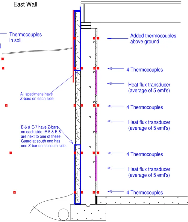
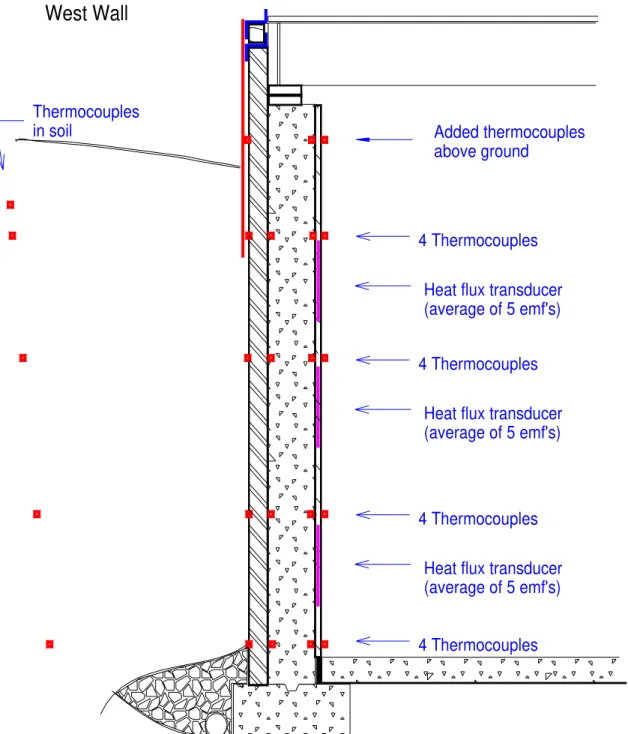
To test and assess the performance of exterior insulation of the basement, different specimens were installed at the exterior of the wall. There were 8 specimens in both walls (east and west) covering a whole wall with approximately 76-mm thickness and 2.44 height, and placed side-by-side. As well, ‘guard specimens’ were installed at each extremity of the two walls (4 specimens in total). On the inside of basement wall, a 25-mm layer of thermally calibrated EPS (expanded polystyrene) board insulation was installed over the entire surface. The thermocouples were systematically placed at the surface of each element in the wall, in a vertical array consisting of 16 points per specimen in the below-grade and 3 above-grade plus thermocouples on each metal Z-bar at the east wall. There were 3 heat flux transducers placed at 3 vertical location on the interior wall. The configurations are shown in figures 1a and 1b. The dimensions and the locations on the wall are shown in figures 2a and 2b.

This thermally calibrated insulation was used to determine heat flux going into the basement wall.

In addition to the temperature measurements, four separate soil analyses were performed to characterise the soil environment, including a vertical profile of moisture content. This information was used to qualify differences in thermal performance of specimens (reported in the main EIBS reports 1,2,3,4).

Installation description

The experimental set up was installed at Test Hut #1 on NRC’s Montreal Road Campus in Ottawa.

Test Hut #1

Installation and instrumentation of specimens

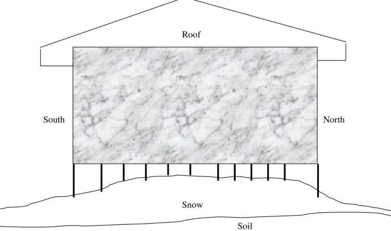
Test Hut #1 has outer dimensions of 2.44 m x 9.144 m, providing about 22.31 m² of east and west walls combined, to be used for insulation studies. Several specimens were placed along each wall (see figure 1a and 1b), (8 specimens), 2 insulation guards were placed at the north and south of the wall. From north to south, the specimens are identified according to insulation:

East Wall:

EPS-C, EPS-B, EPS-C, EPS-C, EPS-A (wrapped in poly), SPF, MFI, & GFI. West Wall:

EPS-B, EPS-B, EPS-C, EPS-C, EPS-B (three 25 mm layers wrapped in poly), SPF, MFI, & GFI.

In the East Side the specimens were labelled E1, E2, E3, E4, E5, E6, E7, E8 and the West Side there were labelled W1, W2, W3, W4, W5, W6, W7, and W8.

Figure 4 illustrates a plan view of the EIBS monitoring set-up at Test Hut #1.

All specimens were fully instrumented excepted for E1, E4 and W1, which were instrumented only at mid-height position.

As well, all specimens were instrumented with heat flux meters in three vertical position except specimen W4 which was instrumented only at the middle vertical position.

The west wall installation featured a cantilevered cementitious board that covered the specimens above-grade. The ground at the west wall was sloped towards the wall at a 5% grade. The east wall cementitious board was supported by metal Z-bars placed between samples and fastened directly to the concrete. The grade on the East Side was sloped 5% away from the wall.

Data acquisition

The data collection was done through an automated data acquisition 6 ½ digit and scanning system, using a multimeter module with high precision, which measures thermocouples, thermopiles and relative humidity sensors. All thermocouples and power signals were routed through a HP command module (HP E1406), which was connected to a PC 486/50.

HP Data acquisition software package (HP-VEE) was used to program the data acquisition routines:

• Wall thermocouples were averaged every 10 minutes, • Soil thermocouples were averaged every 30 minutes.

All measurements were taken every 2 minutes. For the wall thermocouples, 5 readings were averaged every 10 minutes. For the soil thermocouples, 15 readings were averaged every 30 minutes.

This information was stored on PC hard drive as well as floppy disks weekly, in text formatted files, comma-delimited, with column headers showing thermocouples #, date and time for each set of readings. For more information on data organization, see Appendix B.

There were 18 initial files, with 6 additional files for the added thermocouples.

Duration of the field assessment

The first data acquisition system was commissioned in the spring of 1996 and official monitoring started on June 5, 1996. The additional thermocouples on the above-grade portion of the specimens were installed in summer of 1997. The HP-VEE program was modified to store the additional thermocouple readings in separate files. The updated version of data acquisition program was commissioned on August 1997 and official monitoring started on September 29, 1997. The monitoring ended in June 1998 - 2 full years of monitoring.

Instrumentation

The parameters monitored in the EIBS were:

1. Surface temperatures, on both sides of the reference, the concrete and the specimens. 2. Heat flux across the calibrated interior insulation layer (Reference).

3. Soil temperatures from 1 to 2 m away from the specimens, and at 5 depths 4. Interior basement air temperature (average of 4 readings),

5. Exterior air temperature (at north face, shielded from sun), 6. Relative humidity (RH) of indoor and outdoor environment.

The instrumentation package consisted of approximately 275 thermocouples and 81 additional thermocouples, 2 RH sensors, 21 site-built EMF sensors and calibrated heat flux transducers, 4 junction boxes, a data acquisition unit and computer. (For the configuration of the additional thermocouples see Appendix A).

Screen displays of configuration sketches with instantaneous readings of temperatures mapped into these were used as a first level of quality control of the data. These were used for commissioning, debugging and ongoing quality review of the data. The following notes describe the methods of sensing the thermal environmental and the instruments used.

METHODS Temperature

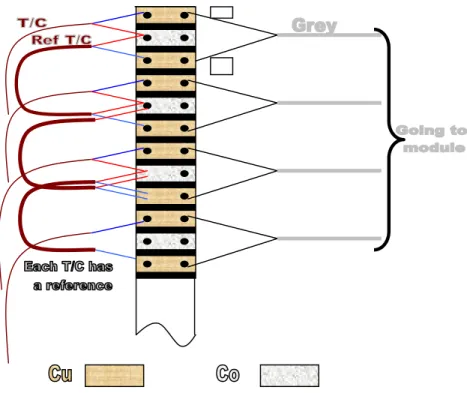
Temperature sensing was carried out using thermocouples. For the EIBS, 30 gauge, type T thermocouple wire was used (TEX/TEX-30-TT). All thermocouples were connected to terminal strips mounted in four sheet metal boxes of 24”x24”x6” in dimensions. Each thermocouple had a copper/constantan/copper terminal. This way connection at the module is done with Cu-Cu wire thus eliminating error caused by dissimilar metal junction (see figure 5).

Figure 5- Schematic Diagram of Thermocouple Junction Box. (Shown are thermocouples, their references and their connection to the module)

Heat flux

All specimens were instrumented with a site-built heat flux transducer consisting of a calibrated sample of 25 mm EPS and five pairs T-Ci sensors for accurate temperature difference measurement. They were placed in the three vertical positions excepted the specimen W4 which was instrumented only at the middle vertical position.

The configuration of the east wall for the heat flux meter placement is shown in the figure 6. The heat flux across this specimen is calculated using a 4th order polynomial function.

In addition to the thermocouples installed on the walls, other sensors and thermocouples were placed to monitor the surrounding environment: indoor and outdoor air temperature and RH.

Relative humidity

Two RH sensors were used – one placed at central location in the basement, the other outdoors on the north wall below the eaves.

Interior basement air temperature (average of 4 readings),

The indoor air temperature is calculated as the average of 4 thermocouples placed inside the Hut#1 in each corner and 1.5 m above floor.

Exterior air temperature (at north face, shielded from sun),

This thermocouple was shielded from the sun and placed at the north face of the Hut#1.

Results and analysis

In the previous sections, a description of the equipment and the testing methodology was presented. In this section, results are presented and discussed.

Data analysis

The data was organised in data file for each week. The weekly data records temperature histories for:

Reference inside surface for the 5 locations (bottom, low, middle, high and top), Concrete inside surface for the 5 locations,

Concrete outside surface for the 4 locations (bottom, low, middle and high), Insulation outside surface for the 5 locations,

Soil temperature at the specimens/soil interface,

Soil temperature placed at 2 m away from the east wall and 10 m away, Indoor and outdoor temperature and RH.

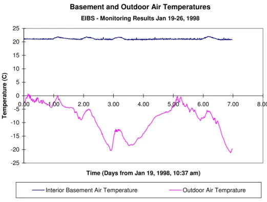
To illustrate a typical cold week of data, week 93 was chosen, from January 16 to January 26, 1998.

Figure 7 shows the indoor and outdoor air temperature profiles versus time. The time period is 1 week, plotted every 10 minutes.

The interior air temperature was controlled and maintained at 23°C and the exterior thermocouple shows temperature. That week, the maximum outdoor air temperature was around 0°C and the minimum was around -20°C.

Basement and Outdoor Air Temperatures

-25 -20 -15 -10 -5 0 5 10 15 20 25 0.00 1.00 2.00 3.00 4.00 5.00 6.00 7.00 8.00

Time (Days from Jan 19, 1998, 10:37 am)

Temperature (C)

Interior Basement Air Temperature Outdoor Air Temprature

EIBS - Monitoring Results Jan 19-26, 1998

West Side

Specimen W5

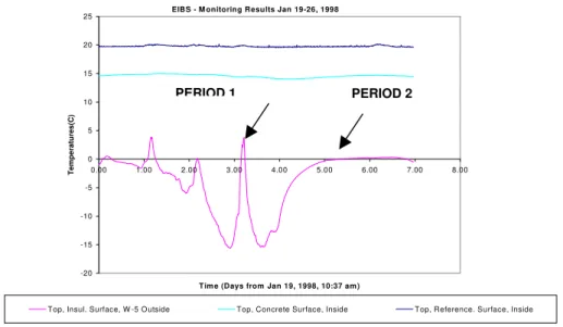
The following figures illustrate the temperature history in the top position for the specimen W5, the west-south guard, specimen E5 and the east-south guard.

The Figure 8 represents the top outside insulation surface temperature of the specimen W5, the concrete temperature inside and the reference temperature inside. The latter 2 temperatures stayed relatively constant in time and were respectively 20°C and 14.5°C. The outside insulation temperature of the specimen follows the profile of outdoor temperature, excepted in 2 periods as shown in this figure, period 1 and 2.

East W all, Sam ple W -5, Top Position

-20 -15 -10 -5 0 5 10 15 20 25 0.00 1.00 2.00 3.00 4.00 5.00 6.00 7.00 8.00

Tim e (Days from Jan 19, 1998, 10:37 am )

Temperatures(C)

Top, Insul. Surface, W -5 Outside Top, Concrete Surface, Inside Top, Reference. Surface, Inside

EIBS - M onitoring Results Jan 19-26, 1998

PERIOD 2 PERIOD 1

Figure 8- Temperatures at Top position for specimen W5

Those 2 periods were the consequence of snow clearance near the wall for a distance between of about 2 feet. In this part the snow was not in contact with the thermocouple, and in the afternoon when the sun heated the wall, it hit directly the thermocouple on the top surface (see figure 9), increasing the temperature for that time period.

Reference-Concrete-Specimen

2’

Snow

Indoor Soil

Figure 9- Lateral view of the wall

The same observations were made on the south guard. The temperature profile is represented in figure 10.

West Wall, Guard South, Top Position

-20 -15 -10 -5 0 5 10 15 20 25 0 1 2 3 4 5 6 7 8

Time (Days from Jan 19, 1998, 10:37 am)

Temper

at

ur

es(

C)

Top, Insul. Surface, Outside Top, Reference Surface, Inside

EIBS - Monitoring Results Jan 19-26, 1998

PERIOD 2 PERIOD 1

East Side

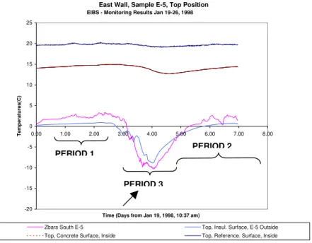
Specimen E5

Figure 11 represents 1 week of the temperature evolution on the metal Z-bar, the outside insulation, the concrete inside and the reference inside versus time period, which is 1 week, and with 10 minutes time step recording. The temperatures are similar to those of top position of the previous graphs. Specimens E5 and W5 are the same product and have the same dimensions. The West face is mirror image of the East face. However, one difference between the East and the West Side is that the East Side has metal Z-bars placed between samples, which are fastened directly to the concrete.

East Wall, Sample E-5, Top Position

-20 -15 -10 -5 0 5 10 15 20 25 0.00 1.00 2.00 3.00 4.00 5.00 6.00 7.00 8.00

Time (Days from Jan 19, 1998, 10:37 am)

T e mp erat u res( C )

Zbars South E-5 Top, Insul. Surface, E-5 Outside Top, Concrete Surface, Inside Top, Reference. Surface, Inside

EIBS - Monitoring Results Jan 19-26, 1998

PERIOD 1

PERIOD 3

PERIOD 2

Figure 11- Temperatures at Top position for specimen E5

The reference and the concrete temperatures are nearly constant, except for the concrete (Period 3), where the temperature decreases (1°C) in the 4th day of the week. The exterior temperature, which decreases considerably, can explain this and it drops to -20°C, as

shown in the figure below. The specimen surface temperature also drops, which is normal.

The profiles of the outside specimen and the Z-bar temperatures compared to the outdoor temperature have 2 anomalies (period 1 and 2). Those profiles don’t follow closely the exterior temperature. The temperatures are above 0°C while the exterior is under 0°C. This is explained by the fact that the specimens were covered partially in this side but the end wall still exposed to the air, so, the thermocouples were heated directly by the sun (see figure 12). For this reason the temperature at the Top position stayed above 0°C.

Roof

South North

Snow

Soil

Figure 13 represents the temperature of the metal Z-bar, the insulation inside and the inside reference of the south-guard at the top position are presented.

The curves respond well to the exterior temperature and have the same shape. A difference of 3°C between the 2 metal Z-bar installed in each edge of the specimen becomes much higher when the exterior temperature decrease considerably. This can be explained by the specimen exposure to the snow as shown in Figure 12, and the especially to the conductivity of the metal.

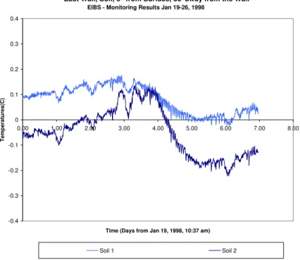
Figure 14 shows the temperatures of the 2 thermocouples placed at 30 ft from the East wall and at 6’’ deep are presented. The difference between the 2 thermocouples is that, one was wrapped and the other was exposed. The profiles of those temperatures are nearly the same for the error that can be made by the thermocouple, which is around ± 0.2°C.

The most important information of this graph is that the soil temperature was equal to 0°C ± 0.2°C, in spite of exterior temperature, which reached –20°C. It seems that the negative temperature of the outdoors air doesn’t affect the soil. In certain weeks the soil temperature dropped to only – 0.8 °C, which is the lowest of the soil temperature at that location for the year.

Figure 13- Temperatures at Top position for the guard

Figure 14- Temperatures of soil

East Wall, Guard South, Top Position

-15 -10 -5 0 5 10 15 20 25 0.00 1.00 2.00 3.00 4.00 5.00 6.00 7.00 8.00

Time (Days from Jan 19, 1998, 10:37 am)

T

e

mperatu

res(C

)

Zbars North Guard Top, Insul. Surface, Outside Zbars South Guard Top, Reference Surface, Inside

EIBS - Monitoring Results Jan 19-26, 1998

East Wall, Soil, 6" from Surface, 30' away from the Wall

-0.4 -0.3 -0.2 -0.1 0 0.1 0.2 0.3 0.4 0.00 1.00 2.00 3.00 4.00 5.00 6.00 7.00 8.00

Time (Days from Jan 19, 1998, 10:37 am)

T e m p er atur es(C ) Soil 1 Soil 2

CONCLUSION

The aim of this study was to explore surface temperatures of the basement wall above-grade to give an overview on the performance of exterior insulated wall above-above-grade. This progress report presented preliminary results based on collected data. Explanations of some apparent anomalies have been presented. The results clearly show that the heat fluxes above grade are a result of important influences such as solar gains, thermal bridges from the metal studs and snow cover. All of these factors will indirectly affect below grade performance, since the concrete within the wall conducts heat above and below grade easily as conditions change.

The final analyses of these results are part of separate papers, which include the assessment of the heat flow along the wall and the orientation of this heat flux in the wall as function of time5,6.

REFERENCES

1. Swinton, M.C.; Bomberg, M.T.; Maref, W.; Normandin, N.; Marchand, R.G. In-Situ Performance Evaluation of Exterior Insulation Basement System (EIBS) - EPS Specimens, pp. 40, 1999 (A3132.1)

2. Swinton, M.C.; Bomberg, M.T.; Maref, W.; Normandin, N.; Marchand, R.G. In-Situ Performance Evaluation of Exterior Insulation Basement System (EIBS) – Spray Polyurethane Foam, pp. 33, 2000 (A3132.3)

3. Swinton, M.C.; Bomberg, M.T.; Maref, W.; Normandin, N.; Marchand, R.G. In-Situ Performance Evaluation of Exterior Insulation Basement System (EIBS) - Glass Fibre Specimens, pp. 35, 2000 (A3129.1)

4. Swinton, M.C.; Bomberg, M.T.; Maref, W.; Normandin, N.; Marchand, R.G. In-Situ Performance Evaluation of Exterior Insulation Basement System (EIBS) - Mineral Fibre Specimens, pp. 35, 2000 (A3129.2)

5. Swinton, M.C.; Bomberg, M.T.; Kumaran, M.K.; Maref, W. "In-situ performance of expanded molded polystyrene in the exterior insulation basement systems (EIBS)". Vol. 23, Journal of Thermal Envelope and Building Science pp. 173-198. Oct 1999. (NRCC-43679)

6. Maref, W.; Swinton, M.C.; Kumaran, M.K.; Bomberg, M.T. "3-D analysis of thermal resistance of exterior basement insulation systems (EIBS)". Journal of Building and

E-6 & E-7 have Z-bars on each side; E-5 & E-8 are next to one of these. Guard at south end has one Z-bar on its south side. All specimens have Z-bars on each side

Thermocouples in soil

East Wall

Heat flux transducer (average of 5 emf's)

Heat flux transducer (average of 5 emf's) 4 Thermocouples

4 Thermocouples Heat flux transducer (average of 5 emf's) 4 Thermocouples

4 Thermocouples Added thermocouples above ground

Thermocouples in soil

West Wall

Heat flux transducer (average of 5 emf's)

Heat flux transducer (average of 5 emf's) 4 Thermocouples

4 Thermocouples Heat flux transducer (average of 5 emf's) 4 Thermocouples

4 Thermocouples Added thermocouples above ground

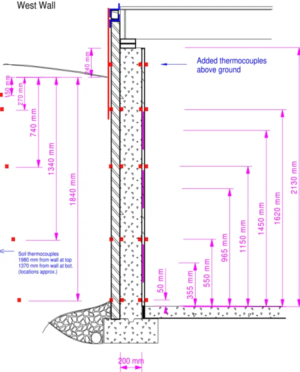
200 mm 18 40 m m 13 40 m m Soil thermocouples 1980 mm from wall at top 1370 mm from wall at bot. (locations approx.) 150 m m 740 m m 2 70 m m West Wall 24 0 m m 2130 m m 1620 m m 1 450 m m 11 50 m m 50 m m 550 m m 965 m m 35 5 m m Added thermocouples above ground

200 mm 18 4 0 m m 1340 m m Soil thermocouples 1980 mm from wall at top 1370 mm from wall at bot. (locations approx.) 150 m m 740 m m 270 m m East Wall 240 m m 2 130 m m 1 620 m m 1 450 m m 1 150 m m 50 m m 5 50 m m 96 5 m m 3 55 m m 12 0 m m

APPENDIX A- EIBS ADDITIONAL THERMOCOUPLES INSTALLED

ON SUMMER OF 1997

South-east Corner Wall

5 Thermocouples (Top, High, Middle, Low, Bottom) on the Guard (Exterior) ◊ Excavation required

5 Thermocouples on the Reference Inside (opposite the guard, on the Interior)

Along East Wall

1 Thermocouple on E-4 outside (Top, middle of Specimen)

8 Thermocouples on Reference Outside (opposite Top, middle Specimens) 8 Thermocouples on Reference Inside (from damaged Thermocouple port) 6 Thermocouples on the Z-Bars remaining (Top, Exterior).

South-west Corner Wall

5 Thermocouples (Top, High, Middle, Low, Bottom) on the Guard (Exterior) ◊ Excavation required

5 Thermocouples on the Reference Inside (opposite the guard, on the Interior)

Soil

1 Thermocouple in soil, far away the basement

The 8 thermocouples in the South East + South West corner will require excavation

Existing additional Thermocouple already installed

12 Tc. installed on East side @ 120 mm above ground

8 Tc. installed on Reference Inside (West) + 8 Tc. installed on Reference Outside (West)

Arrangement of Insulation Specimens Along The Exterior of the West Wall (looking Westward)

Arrangement of Insulation Specimens Along The Exterior of

the East Wall (looking Westward)

West Wall East Wall

EIBS Monitoring Setup At Test Hut #1 (Plan View) 7.010 m 8.230 m 9.114 m 5.791 m 0.305 m W-1 W-2 W-3 W-4 W-5 (wrapped) E-1 1.524 m 2.134 m 3.353 m 4.572 m 2.743 m 0.914 m E-4

E-2 E-3 E-5

(wrapped) W-7 W-6 W-8 E-7 E-6 E-8 4 additional Z-bars at bottom

As Analysed:

A3129/32 8-Jun-98

ID # Material Top High Middle Low Bottom

East face Cement. Board, North Insul. Outside Conc. Inside Ref. Inside Conc. Outside Cement. Board, South Ref. Inside Insul. Exter. Ref. Inside. Insul. Exter. Ref. Inside. Insul. Exter. Ref. Inside. Insul. Exter. At 6" from Soil Surface, and 31' 2" Away from Wall E-1 EPS -B 700 701 702 703 E-2 EPS - B 704 705 706 707 E-3 EPS - C 708 709 710 711 E-4 EPS - C 713 714 715 716 E-5 EPS - A 717 718 719 720 E-6 SPF 721 722 723 724 E-7 MFI 725 726 727 728 E-8 GFI 729 730 731 732 Guard 733 738 740 739 741 737 742 736 743 735 744 734 Soil 745 & 746 West face W-1 EPS -B 757 118 144 443 W-2 EPS - B 758 146 211 W-3 EPS - C 759 213 229 W-4 EPS - C 760 237 244 W-5 EPS - B 761 154 161

W-6 SPF 762 162 100

W-7 MFI 763 312 261

W-8 GFI 451 200 354 450

APPENDIX B- EIBS INSTRUMENTATION RECORD - TEST HUT #1

Number of Items

Description Product ID # Location Calibration Accuracy/ Resolution ISO record

Comments

Data Acquisition

1 Hewlett Packard mainframe data acquisition system, C-size VXI

HP E1401B Test Hut #1, main floor

N/A • Total slot capacity: 13

• Total sensor capacity: a max.of 11cards x 64 outputs

1 HP Command Module HP E1406 HP Slot #0 N/A • Used to translate commands from other modules

• Provides the VXI with resource management cap.

1 Multimeter module HP E1411B HP Slot #1 • measures thermocouples, thermopiles and RH sensors

7 64 channel, 3-wire multiplexer modules HP E1476A HP Slots 2-7 and 9

• interface between sensor and multimeter – provides temperature compensation through onboard thermistor (ref. block)

1 4 channel counter/totalizer module HP E1332A HP Slot #8 • for continual signal monitoring and totaling (4 rain gauges)

1 PC 486/50 Computer & Monitor NHC Test Hut #1, main floor, connected to HP data acquisition

• Hard Drive capacity 248 MB: (holds all the data)

• Self booting after power failures

• Data file opened and closed every reading for proofing against power failures.

1 HP Data Acquisition software package Programmed by Roger Marchand Date: Spring’96

Modified: Sept ‘97

HP-VEE PC hard drive C:\ vee_user Under subdirec. hut

• Used to program the data acquisition routines:

-wall thermocouple: every 10 minutes -soil thermocouples: every 30 minutes -rain gauges: continuous, totaled every 30

minutes, recorded and reset scan rate: sensors/sec:1 reading/2 min

Number of Items

Description Product ID # Location Calibration Accuracy/ Resolution ISO record

Comments

DATA ACQUISITION (CONTINUED)

1 Printer • for record of verification and review

5 Thermocouple junction boxes wall mounted

next to acquisition system

Improves sensor accuracy

Sensors ~55 Thermocouples – ground make/length: ~50 ft All t/c from Thermo- Electric Co. Uncertainty of calibration is ± 0.2°C

Original set. Installed: Fall’95

4 Thermocouples – air make/length: ~30 ft basement, main floor, outdoor (north wall) Uncertainty of calibration is ± 0.2°C

Original set. Installed: Fall’95

? thermocouples – ground/specimen make/length: ~50 ft Uncertainty of calibration is ± 0.2°C

1st summer repair: Installed: June’96

81 thermocouples – ground/specimen/ & above grade make/length: ~50 ft Uncertainty of calibration is ± 0.2°C

2nd summer additions installed:Aug’97

2 RH sensors make: General Eastern RHT-2-I-O/A -20F to 140F

basement &

outdoor (north wall)

± 2%

4 Rain gauges – custom-built basement

floor, south wall

Number of Items

Description Product ID # Location Calibration Accuracy/ Resolution ISO record

Comments

1 Campbell Scientific probe connected to CR10 data logger (CS) CS615 water content reflectometer probe East side-3 ft in ground 2 readings per day

Provides a volumetric water content

Data Files Produced

24 Text formatted files, coma-delimited, with column headers showing

thermocouple #; date and time for each set of readings.

(Approx. 168 Kbytes each)

ASCII text PC hard drive c:\hut_hist & 1.4 MB disks 3 decimal points recorded in Celsius

• coded file names which show end-date and specimen ID