Risk management of drilling waste discharges in the marine environment - a holistic approach

Publisher’s version / Version de l'éditeur:

Oceanic Engineering International, 7, 1, pp. 1-22, 2003-01-01

READ THESE TERMS AND CONDITIONS CAREFULLY BEFORE USING THIS WEBSITE. https://nrc-publications.canada.ca/eng/copyright

Vous avez des questions? Nous pouvons vous aider. Pour communiquer directement avec un auteur, consultez la

première page de la revue dans laquelle son article a été publié afin de trouver ses coordonnées. Si vous n’arrivez pas à les repérer, communiquez avec nous à PublicationsArchive-ArchivesPublications@nrc-cnrc.gc.ca.

Questions? Contact the NRC Publications Archive team at

PublicationsArchive-ArchivesPublications@nrc-cnrc.gc.ca. If you wish to email the authors directly, please see the first page of the publication for their contact information.

NRC Publications Archive

Archives des publications du CNRC

This publication could be one of several versions: author’s original, accepted manuscript or the publisher’s version. / La version de cette publication peut être l’une des suivantes : la version prépublication de l’auteur, la version acceptée du manuscrit ou la version de l’éditeur.

Access and use of this website and the material on it are subject to the Terms and Conditions set forth at

Risk management of drilling waste discharges in the marine

environment - a holistic approach

Sadiq, R.; Husain, T.; Veitch, B.; Bose, N.

https://publications-cnrc.canada.ca/fra/droits

L’accès à ce site Web et l’utilisation de son contenu sont assujettis aux conditions présentées dans le site LISEZ CES CONDITIONS ATTENTIVEMENT AVANT D’UTILISER CE SITE WEB.

NRC Publications Record / Notice d'Archives des publications de CNRC:

https://nrc-publications.canada.ca/eng/view/object/?id=cd7bc907-fdd8-41f3-b939-4b0c14672cd9 https://publications-cnrc.canada.ca/fra/voir/objet/?id=cd7bc907-fdd8-41f3-b939-4b0c14672cd9

http://www.nrc-cnrc.gc.ca/irc

Risk m a na ge m e nt of drilling w a st e disc ha rge s in t he m a rine

e nvironm e nt - a holist ic a pproa c h

N R C C - 4 5 3 8 8

S a d i q , R . ; H u s a i n , T . ; V e i t c h , B . ; B o s e , N .

J a n u a r y 2 0 0 3

A version of this document is published in / Une version de ce document se trouve dans:

Oceanic Engineering International,

7, (1), pp. 1-22, January 01, 2003

The material in this document is covered by the provisions of the Copyright Act, by Canadian laws, policies, regulations and international agreements. Such provisions serve to identify the information source and, in specific instances, to prohibit reproduction of materials without written permission. For more information visit http://laws.justice.gc.ca/en/showtdm/cs/C-42

Les renseignements dans ce document sont protégés par la Loi sur le droit d'auteur, par les lois, les politiques et les règlements du Canada et des accords internationaux. Ces dispositions permettent d'identifier la source de l'information et, dans certains cas, d'interdire la copie de documents sans permission écrite. Pour obtenir de plus amples renseignements : http://lois.justice.gc.ca/fr/showtdm/cs/C-42

".-Risk Management of Drilling Waste Discharges in the Marine

En'vironment - a Holistic Approach

Rehan Sadiq\ Tahir Husain

2,

Brian Veitch

2,

and Neil Bose

2

IInstitute Jor Research in Construction (IRC), National Research Council oj Canada (NRC), 1200 Montreal Road, Ottawa,

Ontario, Canada, KIA OR6

"Faculty oj Engineering and Applied Science, Memorial University ojNewJoundland (MUNj, St. John's, NewJoundland, Canada, AlB 3X5

Email: rehan.sadiq@nrc.ca

ASTRACT

Offshore drilling operations generate wastes associated with rock cuttings and spent drilling fluids during the well drilling phase, The wastes contain toxic substances and are harmful to the marine ecosystem, Discharge limitations and guidelines in different jurisdictions of the world are being developed. Compared to conventional oil·based fluids, the wastes generated from synthetic. based fluids (SBFs) have lower toxicity, lower bioaccumulation potential and faster biodegradation rates, Despite these environmentally benign characteristics, SBF's associated wastes still have a certain amount of pollutants due to contamination with formation oil and the presence of trace heavy metals in barite, which may pose environmental risk. The objectives of this paper are to determine the fate of SBFs waste in the marine environment and integrate methodologies of ecological and human health risk assessment using a holistic risk management modeL Various discharge options representing different treatment levels are used to make a risk-cost trade·off analysis to illustrate the risk management process,

A steady state non·equilibrium water·sediment interaction fate model with probabilistic input parameters was used to determine the concentration of pollutants in sediment pore water. A chemical specific approach was used in the fate modeling, The total toxicity of the drilling waste depends on the toxicity of its individual constituents (base fluid, heavy metals, and organic pollutants). Barite contributes most significantly to the toxicity of drilling waste, The environmental risk assessment for the ecological community and human health was determined' based on contaminant fate modeling exposure concentrations, Uncertainty in the quantification of risks was incorporated into multi·criteria decision·making (MCDM), The risks to the marine ecological community and humans were converted into an environmental risk index, which was then compared to the costs of different offshore treatment options, and of loss due to ecological damage, An analytical hierarchy process using fuzzy composite progranuning was employed to determine the best management alternative for the discharge of drilling waste in the marine

environment.

Key words: Offshore, drilling waste, SBFs, fate modeling, fuzzy composite programming, ecological and human health risk

assessments.

L INTRODUCTION

Demand for energy sources is increasing throughout the world at a rapid rate due to industrial development and population growth, The increasing energy demands have accelerated the search for new sources of oil and gas on land and offshore, Oil production involves two main phases of drilling operations, namely exploration and development. The

exploration phase operations determine the potential hydrocarbon reserves, whereas the development phase operations include drilling of production wells, once a hydrocarbon reserve has already been discovered and delineated, The rigs used in exploration and development sometimes differ but the drilling process is generally the same for both types of operations [U.s, EPA 1999a].

Drilling operations use drilling muds to lubricate the drill bit, control borehole pressure, and flush rock cuttings out of

ｾｬＧ［

,

:"

the well, Disposal of rock cuttings and used mud constitutes one of the most significant waste discharges associated with offshore drilling, The drilling fluids, or circulating muds, are r" broadly classified into three groups,

I., Water-based drilling fluid (WBF): conventional drilling mud with water as a base fluid

2, Oil-based drilling fluid (OBF): diesel, mineral, or some other oil as its continuous phase

3, Synthetic-based drilling fluid (SBF): synthetic material like polyesters and vegetable esters as its continuous phase The SBF mud system consists of a synthetic base fluid, weighting agent (barite) and some other additives, Since 1990, the oil and gas extraction industry has developed many synthetic and non-synthetic materials as base fluids to provide drilling performance characteristics comparable to traditional OBFs with the lower environmental impacts and greater worker safety of WBFs, These characteristics have been achieved through lower toxicity, elimination of polynuclear aromatic hydrocarbons (pAHs), faster biodegradation rate, and lower bioaccumulation potential of pollutants [U,S, EPA 1999a],

The discharge of OBF rock cuttings into the North Sea has been prohibited by the Norwegian regulatory authority, As a result, all such cuttings must be either re-uuected downhole, or shipped to the shore for treatment and disposal. Discharge of SBFs is restricted and is pennitted only on a case by case basis, The regulatory authorities on the East Coast of Canada have recently moved from 15% (by dry weight) drilling muds on cuttings allowed at discharge to a target of 6,9% (on wet cuttings),

The United States Environmental Protection Agency (U.S. EPA) has identified different options to reduce the discharge of drilling waste into the marine environment. Current industry practice for managing and treating SBF cuttings before discharge is to process the cuttings through solids separation equipment, which consists of primary and secondary shale shakers and occasionally a centrifuge. Based on current industry data, the efficiency of ｳｯｬｩｾ separation equipment results in a long-term average of 10.2% (by wet weight) retention on cuttings. However, using new treatment technology, the retention of fluids can be reduced to approximately 4% under certain conditions [U.S. EPA 2000a;2000b].

The disposal of drilling fluids in the ocean environment is of major concern for two main reasons: economical loss associated with expensive synthetic drilling fluid discharged with rock cuttings and probable adverse ecological impacts. To determine the fate of contaminants associated with drilling waste, several studies have been conducted in the past. The U.S. EPA [2000a] developed a methodology for assessing surface water and pore water quality impacts by using the Offshore Operator's Committee (OOC) model as described by Brandsma [1996]. In this analysis it is assumed that discharged contaminants immediately leach into the water column or into the pore water, Instead of SBFs waste as a whole, constituent organic priority pollutants and heavy metals were studied in this analysis. Some other modeling attempts have been conducted based on particle tracking techniques (e.g.,

Seaconsult [2000]), A set of models for the dispersion and drift of drilling wastes and suspended sediment in the benthic boundary layer has been developed by Hannah ef ai, [1997]

who applied these models to the Georges Bank, Canada. Thibodeaux efal. [1986] developed a model for the fate and transport of chemical contaminants originating from offshore drilling bottom deposits. This model was limited to the transport of the soluble constituents from the cuttings and mud deposits, It does not take into account particulate transport and chemical and biochemical transformations that degrade contaminants within the sediment zone or boundary layer. In the North Sea OSPAR (Oslo and Paris) convention area, the Chemical Hazard Assessment and Risk Management (CHARM) model was developed to help stakeholders, including regulators, operators and chemical suppliers, with a risk management module [Thatcher efai, 1999]. The CHARM model categorizes wastes into different application groups, such as production waters and WBFs. The OBFs and SBFs are not addressed in this model due to limited information on input parameters such as biodegradation and bioaccumulation characteristics.

SBFs are hydrophobic in nature and tend to sink to the bottom with little dispersion. Therefore, the main research focus has been on detennining the toxicity in the sedimentary phase as opposed to the aqueous phase, Many studies, including Candler and Leuterman [1997] and Rabke and Candler [1998], have reported the toxicity response of SBFs for different organisms. In addition to the toxicity of the base fluid, the drilling waste contains organic priority pollutants and heavy metals that adversely affect the ecological community [U.S. EPA 1999a]. The CHARM model calculates ecological risk by taking the ratio of two parameters: the predicted environmental concentration to the predicted no-effect concentration(PEC/PNEC), This method is similar to the U,S, EPA approach where predicted concentration is compared with Federal Water Quality Criteria [U.s. EPA 1999b].

Another aspect of environmental risk assessment of drilling waste is human exposure through consumption of contaminated commercial fish. Marine organisms are exposed to pollutants through direct uptake (bioconcentration) and consumption of lower trophic level organisms (biomagnification), Bioaccumulation of chemicals in aquatic food chains, which is a combined effect of the above two processes, is an important phenomenon in aquatic organisms and affects their predators, especially humans and fish-eating wildlife [Campfens & Mackay 1997]. The consumption of contaminated organisms may pose a threat to human health. A deterministic analysis for human exposure and related non-carcinogenic and non-carcinogenic health risk through consumption of finfish and shrimps is presented in the U,S. EPA studies [I 999b; 2000a].

Cost comparisons of different discharge options for water quality, and in the case of zero discharge the non-water quality environmental impacts, are provided in the U,S, EPA study [2000a]. The risk management module of the CHARM model is not well accepted by stakeholders, although it compares various alternatives for risk reducing measures. The basis of risk management in the CHARM model is to combine the risk

2. FUZZY COMPOSITE PROGRAMMING (PCP) • A RISK MANAGEMENT TECHNIQUE

Decision-making is an integral part of all design and management issues. The main concern in decision-making is tbat decision problems are diverse in nature and usually have conflicting criteria. Many attempts have been made to incorporate tbe uncertainty of attributes into decision-making, which involves probability tbeory and/or fuzzy set tbeory. Fuzzy set tbeory is an important tool for modeling uncertainty or imprecision arising from human perception. Human judgment is involved in decision-making, so a rational approach to decision-making takes into account human subjectivity. A traditional multiple criteria decision-making (MCDM) problem can be expressed in a matrix form

all tbe attlibutes for each alternative; and

2. tbe rank ordering oftbe alternatives according to aggregated scores. These two steps are referred to as fmal rating and ranking order, respectively. In fuzzy MCDM problems, tbe performance scores of tbe alternatives are compared and rank orders of fuzzy numbers are determined, which in some cases is not a trivial task. Botb phases are integral parts of fuzzy MCDM.

(a) Grouping of Attributes

FCP is an extension of compromise programming [Bogardi & Bardossy 1983]. In tbis approach, analytical hierarchy process (AHP) and fuzzy aritbmetic are used. Many researchers have used tbis approach in environmental related issues and risk management problems (e.g., James & Lee [1992]; Lee [1992]; Lee et al. [1991]; and Stansbwy et al. [1989]). A detailed description oftbis technique is given in tbis section. FCP is used to assist decision-makers in solving problems of multiple attributes and conflicting objectives. FCP organizes tbe problem into tbe following format

I. Identification of management alternatives 2. Definition of basic indicators

3. Grouping tbem into more generalized indicators

4. Defining weights, balancing factor, the best and worst values oftbe indicators and .

S. Estimation and ranking oftbe alternatives

FCP is a step-by-step procedure of regrouping a set of various basic indicators to form a single indicator [Bogardi & Bardossy 1983]. FCP may use a composite structure of tbe basic indicators selected for risk management of drilling waste. In addition to cost and technical feasibility, risks to botb human and non-human populations can also be taken as basic indicators. Carcinogenic and non-carcinogenic human healtb and ecological risks can also be considered.

The first step in FCP is tbe normalization of tbe basic indicators. This is necessary because all basic indicators have different units and are difficult to compare in tbeir respective units. At tbe first level, human cancer and non-cancer risks are determined for different contaminants, which are grouped into cancer and non-cancer human risk indices (figure I). Similarly, ecological risks are determined for different contaminants to get ecological risk indices.

At level 2, tbe human health cancer and non-cancer risks are grouped as a human healtb risk index. The level 2 human and ecological risk indices are grouped to form tbe environmental risk at level 3. The same procedure is repeated for tbe cost and tbe technical feasibility of treatment operations. The grouping for different attributes is performed in steps, until we get tbe total risk index, total cost and technical feasibility of operations to make a trade-off analysis among conflicting objectives. This trade-off analysis for different alternatives can be done at all hierarchy levels. The system index value at level 4 represents the contribution of tbe final risk index, total cost and final technical feasibility of operations. Figure I shows tbe framework of FCP in a step-by-step procedure for risk management of drilling waste discharges.

(I)

XI

X

2

XII

X

12

X

₂₁

X

₂₂

of individual substances into a single risk estimate. The several management alternatives can be compared on tbe basis of tbeir cost and risk reduction strategy. Some otber researchers (e.g., Stansbwy

et

al. [1989]) used fuzzy composite programming for management of dredged material, which accommodated conflicting objectives - environmental risk and cost - in tbeir analysis.

To develop a decision support system for management of drilling waste discharges in tbe inarine environment, a risk-based approach

was

planned. This research integrates tbe contaminant fate modeling, ecological and human healtb risk assessment and risk management metbodologies [Sadiq 2000; 2001). A risk management metbodology, fuzzy composite programming (PCP), is formulated and applied to optimize drilling waste discharges as an illustrative case study in tbe following sections.

Where

Ai

=

1,2,...,mare possible courses of action or alternatives Xi

=

I, 2, ..,nare attributes, or performance criteria

Xi}.= performance or rating of alternativeAi witb respect to

attribute or criteriaXi

In real life problems, it is common tbatXi}are not assessed precisely due to unquantifiable, incomplete, and non-?btainable information and partial ignorance. These limitations m MCDM metbods lead to fuzzy-based approaches. To perform MCDM using fuzzy-based metbods, two main steps are followed:

where

n}

=

number of elements in second level group}

Si,hJ (x) ｾ basic value for 1-th basic indicator in the second level group} of basic indicators with membership ofh

wiJ

=

weight reflecting the importance ofeach basic indicator

cr

wiJ= 1) and

The values of the basic indicators can be designated by fuzzy numbers to characterise their uncertainties. By defining Z, (x) as a fuzzy number of the

lh

basic indicator with a triangular membership function of ,u[Z,(x)], various management altematives under uncertainty can be evaluated. The confidence level for an uncertain value can be determined using observed or measured variability. Since units of basic indicators are different, the actual value of each basic indicator should be transformed into an index, S'.h(X), using the best or the worst value of the indicator as shown in figure 2 [Leeet al.

1991]. Using the index values of basic indicators, the level 2 index values,L;'h(x), of composite indicators can be defined by

{

",

r

k }IIIPi)

Li,h(X)= !:W',iLS',h,JXJI;

1",/ ' .

(2)

p} is the balancing factor for group}

Further; the index valuesLk,h(X),of the third level composite indicators can be calculated by using the' index values for the second level composite indicators. This procedure is repeated to the final step, which compares three index values of the 4th level indicators: environmental risk, cost and technical feasibilitY.

The selection of weights (w) and balancing factors (p) depends on a single or group of decision-makers. The weights represent the relative importimce of each indicator as viewed by a decision-maker, whereas the balancing factors account for maximum deviation of the indicators and limit the ability of one indicator to substitute for another. A weighting technique ' is used to group basic indicators into more general groups. The weights are allotted in each group based on their relative importance. The process, called an analytical hierarchy process (AHP), is used to determine the weight of each indicator in a group by a paired comparison of each, of the indicators [Saaty 1988; Lee 1992]. Human health cancer risk Human health risk Human health non-cancer risk Ecological risk Total cost saving index Ease of operation Environmental risk reduction index Status of technology Control measures Level I Technical feasibility

Level II Level III Level IV

S,.•(x) BES>WOR

Z".(X)

;?;

BESZi

WORZi

< Z/J,(

x)

< BESZi

Z".(X);?; WORZi

[ 1Z,.(x)-WORZi] S,.(x)= :EsZi-WORZi b BESZI WORZI • '-_-L----'_-l._-'-

Z".

ｾ c d 1.0 S"h(x) 1.0 d c BES<WOR

1"-I

1\

I

''''-[ 1Z",(x)-WORZi] S",(X)= :ESZi-WORZi

Z".(X)

,,; BESZi

BESZi

< Z".(X) < WORZi

Z,.(X);?; WORZi

BESZI. b WORZI

Figure 2, Transfonning actual value ZI,h(x) into nonnalized index value SI,h(x).

To detennine the ranking for various management alternatives, assume L(x) as a fuzzy number, which is represented by a final composite indicator of alternative x. With the help of two index values,

L._

I (x) and

L._.

(x), the

membership function, ,u[L (x)], of the fuzzy number can be calculated approximately. For m management alternatives there are mfuzzy numbers, [L(x), x

=

I, 2, ... , m], to which any ranking method can be applied. The Chen [1985] ranking method detennines the ranking of m fuzzy numbers by maximizing and minimizing sets. This method has been extensively used in ranking alternative studies [Lee 1992; Stansbury el al. 1989]. The methodology of FCP allows the incorporation of complex social, ecological and economic infonnation into the fuzzy decision-making process. The details of weighting schemes and fuzzy ranking methods are given in the following sections.

(b) Weighting of Basic Attributes

MCDM methods require infonnation about the relative importance of attributes or criteria. Itis usually established by a set of preference weights, which are nonnalized to a sum of

I. Incase"n"criteria, a set of weights can be written as

(3)

•

LW) =1 (4)

)=1

Therefore, the MCDM problem (equationI)becomes

Xl X, _Xn W

AI Xu X12 Xln WI

A, _{X'l X" X'n} W,

D= (5)

Am Xml Xm, Xmn W_n

Saaty [1988] has proposed AHP to .estimate the relative weight of each attribute in a group based on a paired

comparison. To compare criterion ｾＧｩＢ with "j" the

decision-maker can assign values au from table I. He proposed the following steps to assign the weights:

I. Ifay=r,thena)l=(J/r),where

t"

0 andI ..j

2. If1=j,thenau= ajl= I

3. Construct matrix A

=

(ay/I =1.... n;j

=

1.... n)

Itis further shown that the eigen vector corresponding to the maximum eigen value of matrixA is a cardinal ratio scale for the criteria compared [Saaty 1988]. The elgen value problem can be solved by:

Where (/l"""is a scalar corresponding to the maximum eigen " value and the unit vector "W" corresponding to ＨＯｬｭｾ gives the

preference weights.

_,

Intensity of Defmition importance I Equal importance 3 Weak importance 5 Strong importance 7 Demonstrated importance 9 Absolute importance 2,4,6,8 Intermediate values

Table 1. Linguistic measures of importance (Saaty 1988). A double weighting scheme is proposed in FCP. The second type of weighting used in FCP is the balancing factor (P).The balancing factor is assigned to groups of indicators to reflect the importance of the maximal deviations of an indicator value and the corresponding best value for that indicator. The larger the value, the greater is the concern with respect to the maximal deviation. When p = 1, all deviations are equally weighted, for p = 2, each deviation receives its importance in proportion to its maguitude [Torno et al. 1988].

(c) Converting Linguistic Terms into Fuzzy Nurnbers

For those basic indicators that are expressed by linguistic terms (e.g., good, poor or excellent) a numerical approximation is proposed to convert linguistic terms into corresponding fuzzy numbers. Chen and Hwang [1992] have defmed eight scales to convert linguistic terms into fuzzy numbers and one of the most important scales is shown in figure 3. This scale contains five levels. The linguistic terms for this scale are

"very low", "low", "medium", "high", and "very high". The

same linguistic terms may contain different meaning in different scales. The "high" ｾ this scale means [(0.6,0), (0.75,1.0), (0.9,0)], that is, the most likely value (when the membership functionJl"x)is 1) is at 0.75 and the largest likely interval is between 0.6 and 0.9 (when the membership function,Jl"x)is 0). Similarly all other linguistic terms can also be defmed from figure 3.

(d) Converting Statistical Data into Fuzzy Numbers

For those basic indicators that are expressed by statistical data, the most crucial step is to deterruine the membership

functions. There are many guidelines on developing

membership functions for fuzzy sets. The fuzzy sets based on statistics are perhaps one of the most naturally fuzzy sets that can be used [Civanlar & TrusseI1986]. The statistical data can be represented by histograms, which can be used for approximation of a probability density function (PDF). Consequently, the fuzzy sets using this histogram can follow the rule that max[,u (x)] = 1. A similar approach is used by Guyonnet et al. [2000] for comparing MC simulation results

and fuzzy arithmetic as two methods of measuring

uncertainties.

Jooste [2001] developed a simple methodology for risk estimation of co-occurring stressors in an aquatic ecosystem based on fuzzy sets. He used the lowest 5th, median and the highest 95thpercentiles for defining triangular fuzzy numbers. Sadiq [200I] adopted a similar approach for converting probability data into triangular fuzzy numbers. The confidence intervals of the lowest I % and highest 99% were used to defme the largest likely interval of the fuzzy number. The mode of the data was used to define the most likely value of the fuzzy number with a membership function value of 1. Figure 4 shows this methOdology for developing a triangular fuzzy number from statistical data.

...

ｾ

r···-

.

"

.

• •

,

.

0.8 '" , .•...

•

_ 0.6 ｾ

..

0.4 0.2 o.s 0.6 0.4 0.2 ｯｾｾ｟ＭｉＭ｟Ｍｌ｟ＭｬＭ

_ _

---l_--l.._-I-_.L-_-I----l o x

(7)

(L

_{max -}

L

_{mi.) -}

(hi ....

:d,)

(L

_{m", -} C_{i )}

+1

3. RISK MANAGEMENT OF DRILLING WASTE DISCHARGES - A HYPOTHETICAL CASE STUDY

The risk management formulation discussed in this section is now applied to risk management of drilling waste discharges case study. Triangular fUzzynumber _ PDF 99% Values

o

1

Figure 4. Methodology for developing triangular fuzzy number [Sadiq 2001].

(e) Fuzzy Ranking Method in Decision-Making

The alternative performance rating Xij can be crisp, fuzzy, and/or linguistic. When fuzzy data are incorporated into an MCDM problem, the final ratings are no longer crisp numbers, rather they are fuzzy numbers. The fuzzy numbers are not straightforward to compare. In MCDM applications when the fmal ratings are fuzzy, different ranking methods can be used

to compare these fuzzy utility values UT(x). Chen's ranking method [Chen 1985] is extensively used for risk-cost trade-off analysis.

The first step in Chen's ranking method [Chen 1985] is to' estimate the final composite L(x) of alternative Ai. The final index value of the composite system is in the form of fuzzy numbers. With the help of index values, Lh

=

1(x) and

Lh

=

0(x), the membership, "'-x) can be estimated. Chen [1985] has generalized the results for trapezoidal fuzzy numbers as shown in figure 5. The alternative that has the highest ordering valueUT (x)is selected as the best alternative.

The risk management methodology developed above was applied to a hypothetical case study of an oilfield on the East Coast of Canada. The contaminant fate modeling, ecological and human health risk assessment, and cost estimation models were integrated to show the significance of adopting a holistic risk management methodology for the selection of the best management altemaJ;ive for drilling waste disposal in the marine environment.

Various discharge scenarios representing management alternatives were selected based on regulatory discharge requirements and efficiency of state-of-the-art solid control devices. Based on these selected discharge scenarios, the loading rates for contaminants present in the drilling waste stream were estimated. The fate models were employed in estimating the predicted environmental concentration in the pore water. In the next step, the ecological and human health risk assessment models were used for risk characterization, based on estimated exposure concentrations (EC). In the end, a tradeoff analysis was performed to decide the best management alternative for the discharge of drilling waste .from risk reduction, cost saving, and technical feasibility viewpoints. A methodology framework for this integrated approach is shown in figure 6. A step-by-step description of each module is given below.

Figure 5. Chen [1985] ranking method for trapezoidal fuzzy numbers.

"

a,

r..,

Lx

b, d,

(a) Contaminant Fate Modeling

Contaminant fate modeling consi,ts of drilling waste characterization, discharge scenarios definition, estimation of pollutant loading rates and estimation of pollutant concentrations using fugacity/aquivalence models.

(I) Characterization ofDrilling Waste

The waste stream discharged from drilling operations that use SBFs.or other non-aqueous drilling fluids consists of three main components: drilling fluid, drill cuttings, and formation oil. The U.S. EPA [1999a] has analyzed pollutant reduction options, compliance costs, and non-water quality environmental impacts, which are based on the drilling waste characteristics data given in table 2. Formation oil is the only source of organic priority pollutants in the SBF cuttings waste

SBFs contain 47% synthetic base fluid, 33% barite, and 20% water by weight; and 0.2% formation oil ofSBF (by volume)

Priority pollutant organics mg pollutant/ml formation oil

Naphthalene 1.43

Fluorene 0.78

Phenantherene 1.85

Phenol 6.0

Metals mg/kg of barite Metals mg/kg of barite

Arsenic (As) 7.1 Lead (Pb) 35.1

Cadmium (Cd) 1.1 Mercury (Hg) 0.1

Chromium (Cr) 240.0 Nickel (Ni) 13.5

Copper (Cu) 18.7 Zinc (Zn) 200.5

Table 2. Waste characteristics of SBF-cunings.

(ii) Discharge Scenarios and Pollutant Loading Rates

A hypothetical oilfield comprised of 32 wells - and the associated discharge - was considered on the Grand Banks of Newfoundland. The elements of greatest concern in these wastes were base fluid, heavy metals, and formation oil, although the cuttings themselves were also a concern because of their smothering effect on the benthic community. The hypothetical oilfield encompassed an affected area of 67 km2•

ｔｨｾ wells were assumed to be uniformly distributed over that area. The affected impact area(A_w)for a single well was 2.09 km2• The radius of impact area (R) for a single well was approximately 816 m. The depth of the water column was 95m. The welIs were assumed to be drilled' only by SBFs (esters). The esters are the most commonly used and environmentally benign synthetic based drilling fluids [U.S. EPA 2000a]. Pollutant loading rates of heavy metals, base fluid (ester) and organic priority pollutants were calculated based on deep development model well data as suggested by U.S. EPA [2000a; 2000b].

Five discharge scenarios were selected as potential management alternatives for drilling waste disposal in the marine environment. These alternatives included 10% (current practice in Gulf of Mexico), 8.5% (obtainable with the current technology), 7.0%, 5.5% and 4.0% (BAT proposed). These alternatives represent the percentage of base flnid attached to the wet cuttings. Detailed step-by-step procedures are provided in Sadiq [2001] for estimating the amounts of pollutants and base fluid expected to be released into the environinent for

various discharge scenarios. .

The SBF consists of 47% base fluid (ester), 33% barite and 20% water. The density of drilling waste depends on the reservoir rock type and the amount of base fluid attached to the drill cuttings. The major components of drilling wastes are drill

cuttings, base fluid, barite and water. The weights and volumes of these components were calculated based on ester percentage attached to the cuttings. The volume and weight of dry drill cuttings were estimated using borehole volume and the density ofdry cuttings.

The quantities of each component were estimated to determine the weight and volume of total drilling waste for a given discharge option. The total volume of base fluid discharged for the 10% discharge option was estimated to be 57 m' per well. The amount of formation oil was estimated based on an assumption that it is 0.2% volume fraction of the SBF, which is 140 kg for the 10% discharge option. The weight of barite discharged under the 10% discharge option is approximately 32,000 kg. The barite discharged in the marine environment contributes trace heavy metals, which pose a threat to ecological entities.

The amounts of heavy metals depend on the quantity of barite discharged for each option. The effluent concentrations of heavy metals in a drilling waste stream (GE ) were estimated based on the weight fractions of metals in the barite, whereas organic pollutant concentrations depend on the volume fraction of formation oil present in the SBF. The volume fraction of SBF was calculated by dividing the volume of SBF with the total volume of drilling waste for a given discharge optiou [Sadiq 2001].

The total quantities of pollutants were estimated by multiplying the total volume of the drilling waste with the GE of each pollutant present in the drilling waste stream for a given option. An average time of one-month is assumed to estimate the loading rates for each pollutant [U.S. EPA 2000a]. The loading rates calculated for all pollutants are provided in mglhr, except for ester, which is given in kg/hr. Table 3 provides a summary of pollutant loading rates estimated for different discharge scenarios.

Pollutants 10% 8.5% 7.0% 5.5% 4.0% As 311 254 201 152 107 Cd 48 39 31 24 17 Cr 10,495 8,573 6,796 5,146 3,612 Cu 818 668 530 401 282 Hg 4.4 3.6 2.8 2.1 1.5 . Ni 590 482 382 290 203 Pb 1,535 1,254 994 753 528 Zn 8,768 7,162 5,677 4,299 3,018 "'Naphthalene 3319 270/ 214 162 114 °Ester 62 51 40 31 21

"'Naphthalene is considered as the marker for formation oil contamination in the drilling waste. Other PAH are not considered in the analysis *Ester (values are in kg/hr)

Table 3. Pollutant loading rates(E,mgIhr)for one month for different discharge scenarios [Sadiq 2001].

(ill) Application ofFate Models

Generally, physical processes are employed in the fate modeling of drilling waste, however other processes including chemical, biological and ecological are not incorporated. The transport of drilling waste involves advection, dispersion, flocculation, deposition, consolidation, erosion, and resuspension. The impacts of these processes on the fate of drilling waste depend on the characteristics of the waste and the hydrodynamics of the receiving water bodies [Khondaker 2000].

Fugacity/aquivalence based models have been applied for detergent chemicals, PCBs, and heavy metals to determine their fate in rivers and lakes [Mackay 1991]. In these models, a steady state solution descnbes conditions that will be reached after prolonged exposure of the system to constant input conditions. The use of fugacity as an equilibrium criterion is suitable for chemicals that can establish measurable concentrations in the vapor phase.Itis not applicable to some metals, organometals, ionic compounds, or some organics such as polymers whose vapor pressure is negligible. To model the behavior of these chemicals, another equilibrium criterion known as the aqueous equivalent concentration (aquivalence) criterion is used [Mackay & Diamond 1989]. A model developed in terms of aquivalence is ultimiltely similar to models written in terms of concentration or fugacity. Steady state non-equilibrium fugacity and aquivalence models were employed in this study for organics and heavy metals, respectively. The formulation of these models can be seen in Sadiqet al.[2001a-d].

The model inputs were defmed by statistical distributions to incorporate uncertainty and variability. Monte Carlo (MC) simulation is one of the most widely used methodologies to account for parameter variability in contaminant transport and fate modeling. The robustness and capability of MC simulation methods are not limited by the non-linearity of the problem. A Latin Hypercube Sampling (LHS) based MC simulation was used to estimate the concentrations in the water column and

pore water [Sadiq et al. 2000la-d]. The predicted

environmental concentration (PEC) is defmed as the highest 95th percentile value on the cumulative distribution function (CDF) of estimated concentration profile. The PEC values were adjusted for exposure probability (p) and bioavailability (BF) to estimate the exposure concentration (EC) for each pollutant in various discharge scenarios. The bioavailability of

contaminants depends on their physico-chemical

characteristics and ability of receptors to uptake and intake.It is a complex mechanism but for simplicity BF values are assumed based on the dissolved fraction of pollutants. Similarly, exposure probability also depends on receptor movement and their ability to uptake contaminants. A single exposure probability value was assumed based on the ratio of contaminated area to total area under study. Table 4 summarizes pore water exposure concentrations for various discharge scenarios. These exposure concentrations were used for ecological and human health risk assessments, which are basic indicators in FCP.

Water column concentrations are not reported in this paper as they were below background concentrations due to the hydrophobic nature of drilling waste.

where

Xm = average of the lognonnally transfonned data= 2.85

Sm

=

standard deviation of the lognorrnally transfonned data

=

1.74

Y

=

variable to describe the normal probability

curve

=

Ln (HQ).

value). HQ values greater than 1 represent potential adverse effects. !fthe value is less than I, it means that at least 95% of the ecological community is safe for 90% of the time [Lenwooder al. 1998]. To estimate the probability of adverse effects according to the above criterion, the estimated HQ for each contaminant was converted into a corresponding risk value as suggested by Karmaner al. [1996] and Thatcherer al. [1999] by the following relationship.

(b), Ecological Risk Assessment

The risk characterization of ecological entities is perfonned ｢｡ｳｾ､ on dose response relationships. The estimated dose or exposure was compared with the threshold value of response for each contaminant. The response of the ecological system was detennined based on the lowest lOth percentile value on the PNEC empirical distribution function. The pore water exposure concentration (EC) for each contaminant was used as a representative dose for ecological entities (see table 4). The mean (,ito) and standard deviation (0"10) of response for each pollutant are given in table 5. The response values of each pollutant were used to determine ecological risk estimates separately. The lowest lOth percentile was selected as a threshold level (PNEC criteria value) based on the premise that if exposure concentrations are below this value, there is no risk of adverse effects for the whole ecological community [Sadiq 200 I; Lenwooder al. 1998].

Hazard quotient (HQ) is defmed as the ratio of exposure concentration to the representative response (PNEC criteria

[

.

(Y-Xml]

Ln(HQ) ,

-Risk=

J

.

ｾ･

lSm y=o 8_m 2tr (8) Pollutants 10% 8.5% 7.0% 5.5% 4.0% As 0.23 0.19 0.15 0.11 0.08 Cd 0.17 0.14 0.11 0.08 0.06 Cr 2.05 1.68 1.33 1.01 0.71 Cu 1.01 0.83 0.66 0.50 0.35 Hg 0.00 0.00 0.00 0.00 0.00 Ni 2.01 1.65 1.31 0.99 0.70 Pb 2.19 1.78 1.42 1.07 0.75 Zn 2.35 1.92 1.52 1.16 0.81 Naphthalene 0.00 0.00 0.00 0.00 0.00 Ester 17.68 14.45 11.50 8.70 6.10

Table 4. Exposure concentration in pore water (EC,pglL)for different discharge scenarios. .

Pollutants _Iho 0"10 Pollutants f.l1O 0"10

As 12.12 11.10 Hg 0.075 0.041

Cd 1.87 1.10 Ni 25.82 38.80

Pb 2.12 1.65 Zn 4.24 1.80

Cr 5.77 2.62 Naphthalene 13.04 36.08

Cu 0.20 0.12 Ester 177,475 877,810

Risk (A +B)= Risk (A) +Risk (B)- Risk (A) . Risk (B) (9) The risks estimated for each pollutant were grouped together as statistically independent events i.e.,

,

Similarly,

Risk (A +B+ C)= Risk (A) +Risk (B) +Risk(C)

-Risk (A) . Risk (B) - Risk (B) . Risk (C) - (10)

Risk (A) . Risk (C)+Risk (A) . Risk (B)· Risk (C) And so on..

Thatcher et al. [1999] and Jooste [2000] have adopted similar methodologies for grouping risk in the case of multiple stressors. The risk estimated from equation 8 is in the form of an empirical distribution function (EDF). Therefore composite ecological risks estimated from the series of equations (e.g. equations 9 and 10) are also in the form of an empirical distribution function.

The EDFs of composite ecological risk values were converted into minimum; maXimtfifi likely (mode; MLV)artd maximum values (see figure 4). The minimum, MLV and maximum risk values were used to develop a triangular fuzzy number. Figure 7 shows the minimum, MLV and maximum values for each discharge scenario, where these values represent the lowest I %, mode and the highest 99% of the EDF [Jooste 2001]. The cumulative ecological risk varied over a wide range from 0.18 to 0.63 for the 10% discharge option, with an MLV of 0.26. It reduced to 0.04 to 0.33 for the 4% discharge option with an MLV of 0.13. The base of the triangular fuzzy number represents the uncertainty in the estimates. The apex of the triangle represents the MLV. The highest uncertainty in the ecological risk estimates can be observed for the 10% discharge option and the least uncertainty is observed for the 4.0% discharge scenario. (c) Human Health Risk Assessment

Human health is the other major component of

environmental risk assessment. Human health risk assessment involves exposure through contaminated fish caught at the impacted site. The pore water exposure concentrations (EC) of each contaminant were employed to estimate the fish tissue concentration, which were further used as human exposure concentrations through consumption of contaminated fish. The fish tissue concentration was estimated by multiplying EC by bio-concentration factors (BCF) and lipid content of fish (L,). Human health risk consists of cancer and non-cancer risk estimates. The chronic daily intakes (CD!) were calculated for each contaminant individually. For cancer risk, CD! was multiplied by the slope factor (SF) (arsenic is the only proven human carcinogen in this study) to estimate the unit risk over the life span of a person. Similarly, for the estimation of non-cancer risks, reference doses (RID) were divided by CD! for each contaminant to determine a hazard index HI. In the end, theHIs for all contaminants were summed up to determine the composite hazard index(HI,).

(d) Cost Estimation

The cancer and non-cancer risk estimates are reported in table 6. The minimum, MLV and maximum values for various discharge scenarios are reported. The minimum values correspond to the lowest I% and maximum values correspond to the highest 99lh percentile value of the estimates, whereas the MLVisthe highest frequency value, which correspondsto

the mode value (see figure 4).

The highest estimated value ofHI, for the 10% discharge scenario was 0.086. This value is approximately 12 times lowerthanthe safety level of1.Similarly, the unit risk values are very small, much lower than I in a million, which is

conventionally used as a regulatory measure for human health risk assessment. Although all scenarios represent safe simations from a human health risk viewpoint, the purpose of this study was to make a comparative evaluation of various discharge scenarios based on risk estimates. Therefore these values were used in the risk management section for comparing the different alternatives.

The cost components considered in this study are treatment cost, cost of drilling fluid lost during discharge, ecological and

human health damage costs. To compare management

alternatives or discharge options, the cost estimates were normalized over one year and values are reported in $/day. The information available for the cost estimates is scant in the literature. The information available is only through published reports, which are not in the public domain. The cost estimation requires judgment and generally the estimates are site specific. The summary of cost estimates for different activities is provided in table 7. A plot of total cost estimates for various discharge scenarios is shown in figure 8. Details of the cost estimation analysis can be seen in Sadiq [2001]. (e) TechnicalFeasibility

The third attribute for risk management is the technical feasibility of the treatment options or management alternatives. The technical feasibility of various alternatives was dermed based on three basic indicators: ease of operation (EO), stalus of the technology (ST), and control measures required (CM). These are not necessarily the only indicators to compare various treatment alternatives; rather they cover the basic information about each treatment option. For example, the ease of operation may include .the total number of hours of operation, capacity of the treatment unit, and exposure of workers to drilling fluid. Similarly, the status of technology can encompass the efficiency of the treatment device, availability of skilled labor, and space requirements. The control measures include maintainability of the treatment units, and safety of workers. All of these sub-indicators need a detailed study to incorporate information from vendors, regulators and literature.

The technical feasibility basic indicators were defined qualitatively. The numerical scores are assigned from 0 to 1. The scales are assumed as fuzzy numbers to incorporate vagueness and fuzziness in human judgment. The MLV of (11)

each scale represents the membership function of I. The base ofthefuzzynumber represents uncertainty in human judgment.

Figure 3 illustrates these five qualitative levels to compare technical feasibility basic indicators.

0.8 ｾ ｾ

ｾ

0.6 ｾ

=

.a

:t

_c

..

0.4

""

e

i

0.2 I I

,

• I

,

,

I

•

I

,

,

I • I

,

,

\

,

_,

\

,

_,

\

,

,

\

,

,

,

,

\

,

\

,

--8.50% --7.00% - - 5.50% -·4.00% 0.2 0.4 Ecological Ri,k 0.6 0.8

Figure 7. Ecological risk estimates for various discharge scenarios.

1.0ｾＭＭＭＭｾｾ｟ｾＭｾｾＭ｟ＭＭＭＭＭＭＬＮＭＭＮＮＮＮＬＮＮＮＭＭＭＭＭＭＬ '5.5% "4.0% -10.0% --8.5% --7.0% 0.8 ＫＭｾｾＭｾｉＭＭＮＭｊｪＡＮＮＭｾＭＭｲｾｾＭＭｬ＾ＮＭｾｾＭＭｾＭＫｾＮＭ 0,2 ＭｬＭＭＭＭＭＭｉｉＭＭｉＭＮｉＭｾ｟｟ｉ｟｟ｾｾｾｾｾ｟ｉ｟ＭｾｾｾＧ｟｟ＫＭＭＧＧ｟ＮＭｾＭＮｾ 1300 1100 900 Total co,t ($Iday) 700

0,0 +-...L.1L ｟｟ｉ｟｟ＭＭＭＭＭＭｬＭＭＭＭＭｾＮＮＮＮＮＮｪＮｾＭＭｾＭ｟ｉ

500

Items Parameter 10.0% 8.5% 7.0% 5.5% 4.0% Min. 0.007 0.005 0.004 0.003 0.002 Non-cancer MLV 0.016 0.014 0.014 0.009 0.005 (HI,) Max. 0.086 0.073 0.062 0.044 0.033 Cancer Min. 1.24x10-1• 9.15X 10-17 8.26X 10-17 6.39x 10-17 4.53x10-17 (Unit risk) MLV 5.54x10.16 4.31 X 10-16 5.18X 10-1• 1.73X 10-1• 1.87X10.1• Max. 3.49x10-" 2.95x10"" 2.35x10"; 1.64x 10-15 _1.16x10-15 Table 6. Hwnan health risk assessment for various scenarios.

Items Parameter 10.0% 8.5% 7.0% 5.5% 4.0% ＨＤＯ､｡ｾＩ Min. 201 235 297 356 413 Treatment MLV 353 437 452 541 587 cost Max. 705 784 792 876 902 Min. 27 21 18 10 7 Ecological MLV 39 41 35 27 20 damage cost Max. 94 83 76 64 50 Economic Min. 245 198 157 119 84 loss due to MLV 339 274 217 165 116 drilling fluid discharge Max. 460 372 295 223 157

Human health damage cost Negligible values of costs are estimated for cancer risk. The non-cancer risk costs are also nedected because the cOmDosite(HI,)is less than I for all cases. Table 7. Cost ($/day) estimates for various discharge scenarios.

Parameters 10.0% 8.5% 7.0"10 5.5% 4.0"10

Status of Technology (ST) 3 3 4 4 4

Ease of Operation (EO) 4 4 4 3 3

Control Measures Requirements (CM) 4 4 4 3 2

Table 8. The qualitative scales assigned to rank technical feasibility indicators. Based on figure 3, the ST, EO and CM were rated for

various discharge scenarios. As described earlier in section 2 (c), this qualitative scaling needs significant infonnation before assigning any scale. The scales were assigned based on a simple comparative evaluation. The scales I and 5 were not assigned for any indicator because the scale I represents a poor level, which is not the case for any altemative. Even in the case of ST, scale I could not be assigned to the 10% discharge option, because it represents a current discharge practice in the U.S. offshore. Similarly, scale 5 represents an excellent level, which could be assigned to EO in the case of the 10% discharge option or for the 4% discharge option for ST. It is avoided because there are some other technologies, like a thermal treatment option, which were not evaluated in this study, but might warrant a better scale rating. Based on these considerations, the scales were assigned to technical feasibility attributes for various discharge options as given above in table 8.

(I) Fuzzy Composite Programming (FCP) (i) Normalization ofBasic Indicators

Figure I showed that at the first level, the human health canCer and non-cancer risks were grouped together to make a human health risk index. Similarly the three basic indicators ease of operation, status of technology, and control measures -were grouped to get the technical feasibility index. At the second level, the human health risk and ecological risk were grouped together to make a general group of the environmental risk reduction index. At the final stage, environmental risk reduction, technical feasibility and total cost saving indices were grouped to obtain a system improvement index.

The higher the risk value the less desirable that alternative will be. Similarly, if the total cost is more, that option will not be desirable. Contrary to that, if some basic indicators have a higher value (e.g., ease of operation), it may considered a better option. To avoid this confusion, all basic indicators were

normalized based on two criteria, either WORST > BEST (e.g., risk, cost etc.) or BEST> WORST (e.g., technical feasibility). These two criteria were used to normalize the basic indicators into unitIess numbers scaling from 0 to I. The method is illustrated in figure 2. The BEST and WORST values were selected among the estimated values for different discharge options.

After defining the BEST and WORST criteria values for each basic indicator, the values were normalized. All normalized basic indicator values were unitIess and were scaled from 0 to 1, in which a higher value meant a better option. The risk and cost estimates became a risk reduction index and a cost saving index, respectively. Table 9 summarizes the normalized values of risk reduction and cost saving indices. The technical feasibility indicators are already scaled from 0 to I. The estimated normalized values of all basic indicators are reported in unitIess terms so that they can be grouped accordingly using FCP methodology.

(il) Weighting Schemes for Basic Indicators

After normalizing the basic indicators, the next step in FCP is to defme the weights for different attributes. A double weighting scheme was used. The first type of weighting (w) is based on one-to-one comparison of attributes. The AHP process defmed the relative importance of each attribute and grouped them into a generalized group. For example, human cancer risk and non-cancer risks were proportioned as 2: 1 by importance, at the first level. Similarly, human health risk was given more priority than ecological risk by giving double weight to human health risk. At the highest level, the environmental risk reduction and cost saving were given three times more weight in comparison to the technical feasibility. Table 10 summarizes the calculated weights for all attributes at various levels. The second type of weight is the balancing factor (P); it was assigned to groups of indicators to show the importance of the maximal deviations [Tornoefal. 1988]. (iii) TradeoffAnalysis

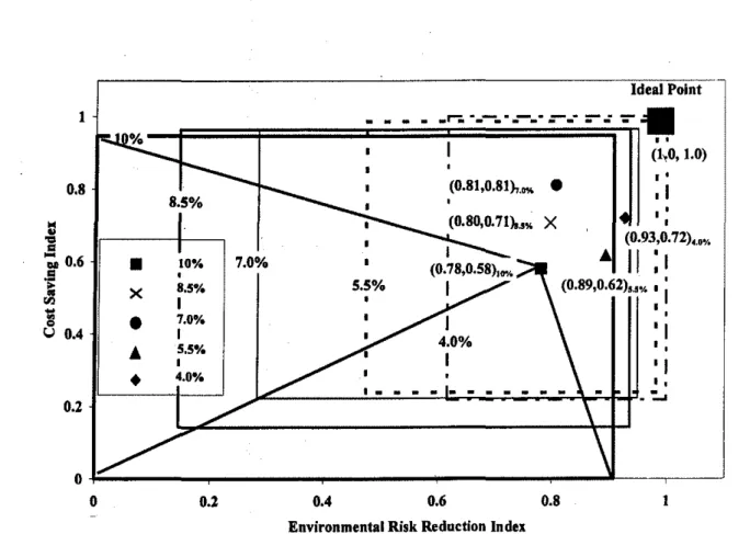
After assigning weights to basic indicators and more generalized groups at higher levels, a tradeoff analysis was performed. The analysis was repeated for each management alternative or discharge option. FCP can be used for comparing two attributes at any level, e.g. at level 3. Figure 9 shows a comparison of the environmental risk reduction and the' cost saving indices for different discharge options.

The plot shows the largest likely interval, or range, of the fuzzy number (base of the triangle, when the membership function, J.lY = 0) in two dimensions. The x,axis shows the largest likely interval, or range, of the environmental risk reduction index and the y-axis shows the largest likely interval of the cost saving index. For the 10% discharge option, the largest likely intervals are joined with the MLV. This can form a pyramid if it is viewed in 3-0. The MLVs of two indices are also provided for each option given by thexandycomponents. The larger base of the pyramid shows higher uncertainty in the indices. The 10% discharge option has the largest base for the cost saving index. The 4% discharge option shows more

uncertainty in the cost saving indexthanthe environmental risk reduction index. The MLV of cost saving and environmental risk reduction indices are at (0.93, 0.72). The ideal point in this type of comparison would be (1.0, 1.0) which is practically very difficult to achieve.

The environmental risk reduction index can also be compared with the technical feasibility index. Figure 10 shows that the base (or largest likely interval) of the 5.5% discharge option is larger than the other options, but the environmental risk reduction index uncertainty is maximum for the 10% discharge option. The 7.0% discharge option shows the best results from a technical feasibility viewpoint. If the system improvement index is based on only technical feasibility and environmental risk reduction viewpoints, then the 7.0% discharge option may be the best option, as its MLV is closest to the ideal point (1.0, 1.0). But this option shows higher uncertainty in the environmental risk reduction index than the 4.0% and 5.5% discharge options. The environmental risk reduction index was assigned three times more weight than the technical feasibility index, which reduces the chance of the 7.0% option to be selected as the best discharge option.

Similarly, the cost saving index can be compared with the technical feasibility index. Figure 11 shows that the 7.0% option is the best option if the cost saving and the technical feasibility indices are the maj or criteria. The MLV of the 7.0% discharge option is closest to the ideal point (1.0, 1.0).

After estimating the technical feasibility, cost saving, and environmental risk reduction indices, they are grouped as a system improvement index. This final index is in the form of a fuzzy number. For all discharge options, the system improvement indices are compared in figure 12. The ideal point of (1.0, 1.0) is also shown for comparison. The 7.0%, 5.5% and 4.0% discharge options look very close to each other. The MLV of the 7.0% and 4.0% discharge options are approximately the same (0.80), but the largest likely interval of the 7.0% discharge option (0.62) is bigger than the 4.0% discharge option (0.51). The larger base represents higher uncertainty in the estimates.

(iv) Ranking Alternatives

Figure 12 shows that selection of the｢･ｾｴ alternative is not an easy task, because some alternatives ate very close to each other. The Chen [1985] ranking method was used to rank these discharge scenarios outlined in section 2(e). In Chen's ranking method [Chen 1985] the utility value U,(x) was determined for each fuzzy number as described before. The highest utility value represents the best management alternative. Table 11 summarizes the system improvement index values for these discharge scenarios. The utility values were calculated for the system improvement index for each scenario. A conclusion can be drawn from this ranking method that the 4.0% is the best management alternative in our hypothetical case study, followed by the 7.0% and then the 5.5% discharge option.

(vi) Sensitivity Analysis

The ranking of various discharge options was the last step in deciding which option is the best management alternative. The

process of ranking alternatives involved assumptions and human judgments for assigning weights to various attributes. To confirm the ranking order achieved in the previous section, sensitivity analysis was performed in which various weighting schemes were employed and the entire FCP procedure was repeated. Table 12 summarizes the trials in which new weights and importance values were assigned to the last three groups. The first trial results have already been discussed in which risk reduction and cost saving indices were given three times more weight than the technical feasibility index. The second trial

represents the case in which technical feasibility is not considered, rather risk reduction and cost saving indices were assumed to be the selection criteria for the best management alternative. Similarly in the third trial, the environmental risk reduction index was given 1.5 times more weight than the cost saving index. This trial represents the pro-environment scenario. In the last trial, the weights of environmental risk

reduction and cost saving indices are reversed, which is a pro· cost saving scenario.

Indicators Values 10.0% 8.5% 7.0% 5.5% 4.0%

HHRo Min. 0.0000 0.1568 0.3309 0.5371 0.6764

(Reduction) _{MLV 0.8523 0.8880 0.8628 0.9629 0.9589}

Human health

cancer risk Max. 0.9772 0.9866 0.9892 0.9946 1.0000

HHR",

Min. 0.0000 0.1514 0.2788 0.5060 0.6370 (Reduction) MLV 0.8329 0.8558 0.8666 0.9207 0.9712 Human health ｮｯｮｾ｣｡ｮ｣･ｲ risk Max. 0.9507 0.9651 0.9772 0.9892 1.0000 ER Min. 0.0000 0.1259 0.2129 0.3487 0.5103 (Reduction) MLV 0.6304 0.6050 0.6781 0.7718 0.8499

Ecological risk _{Max. 0.7723 0.8425 0.8753 0.9605 1.0000}

Min. 0.0000 0.1430 0.2236 0.2383 0.2186 Cost MLV 0.5796 0.7070 0.8110 0.6166 0.7186 (Saving) Max. 0.9469 0.9647 0.9657 0.9870 1.0000 Min. 0.6000 0.6000 0.6000 0.3000 0.3000 EO MLV 0.7500 0.7500 0.7500 0.5000 0.5000 Max. 0.9000 0.9000 0.9000 0.7000 0.7000 Min. 0.3000 0.3000 0.6000 0.6000 0.6000 ST MLV 0.5000 0.5000 0.7500 0.7500 0.7500 Max. 0.7000 0.7000 0.9000 0.9000 0.9000 Min. 0.6000 0.6000 0.6000 0.3000 0.1000 CM MLV 0.7500 0.7500 0.7500 0.5000 0.2500 Max. 0.9000 0.9000 0.9000 0.7000 0.4000

Table 9. Normalized values of the basic indicators used in fuzzy composite programming.

Indicators Importance value w p

Human Cancer Risk 2 0.67

I

Human Non-cancer Risk I 0.33

Human Health Risk 2 0.67

2

Ecological Risk I 0.33

Status of Technology I 0.33

Ease of Operation I 0.33 2

Control Measures Requirements I 0.33

Technical Feasibility I 0.14

Environmental Risk Reduction 3 0.43 2

Cost Saving 3 0.43

.

Ideal Point I

. . .

.

..

r-::-_._._----.

..

..

..

.

..

..

.. .. .. ..

.

,

(1,0,1.0) (0.81,0.81),.",

•

I ' 0.8 I

I

X I ' :I I

...

..

(0.93,0.72)... I

..

II

• I

';'" 0.6

•

10% 7.0% _{(0.78,0.58)'0%}

'5

X

,

8.5% 5.5%

I

(0.89,0.62)..% II

i

'"

_ｾ I I i!l

•

7.0%

_I

,

U 0.4 I _4.0% I

I

..

5.5% I , I

I

_I

I

•

4.0% I , I • _{• ':..0} 0.2 1 0.8 0.6 0.4 0.2

o

ｾ

...,...

I I - - - - , - - _ J

o

Environmental Risk Reduction Index

Figure 9. Comparison of environmental risk reduction and cost saving indices.

Ideal Point 1

•

7.0% - - - ( 1 . 0 , 1 . 0 ) 5.5%. • • • _

ＨＰＺＸＱｾＮ＿ＵＩＮｊ［ｪＮ

• I _ ｾｾＮ I • (0.8, 0.67) ';l .... I (0.78, 0.67) (0.89,0.59) 4.0%

i .;

I (0.93,0.54)

,

-.-

L- ..

...

_---'

-...I " 0.8

i

ｾ

:c; 0.6

!

==10% ｾ - - - , I: 0.4

!

0.2 0.6 0.8

Environmental Risk Reduction Index

Ideal Point

•

ｾＷＮＰＥ (1.0,1.0)

-(0.81,0.75)

-

--

-

-

_-

-

- 5.5% - (0.71,0.67) - •

--

.

..

•

-r. ._. - .

(0.60,0.67)-"- • - •

X . - .

-4.0% •

_{; I}

•

ｾＮＵＥ " ｾ

_•

,

(0.62, 0.59) _

--

' I

II....:

10%

-r

_{I ,}'

.

•

,

(0.72,0.54)

'I

_I 10%

I.

ｾ

-

-

.

-- - -

.

-

.

- -

....

-

.

-

. . . .

-•

｟Ｎ｟Ｎ｟ＮＭＮ｟Ｍ｟ＮＭＮ｟ＮＭＭ｟Ｎ｟Ｎ｟Ｎｾ X 8.5%

•

7.0%

...

5.50;•

•

4.00/.

,

,

I ... 0.8

i

-!

0.6

!

ｾ

..a

0.4

ｾ

0.2

o

o

0.2 0.4 0.6 0.8 1

Cost Saving Index

Figure 11. Comparison of cost saving and technical feasibility indices.

0.8

0.4 0.6

System Improvement Index 0.2 --8.5% --7.0% -10.0% - - 5.5% _ . 4.0% 1 ｲＭＭＭＭＭＮＭＭＭＭＭＭＭＬＭＭＭＭＭＬＮＭＭＭＭＭＮＮＮＭＭＭＭＮＮＭＭｾＭＭＭＭＭｪ

..

(1.0,1.0) I Ideal Point

o

+- ＨＭｌＮＮＭ｟ｌＭｾｉ｟｟ＭｌＭ｟ＮＭＭｊＭＭＭＭＭＭＫＭＭＭｬＮＮＮｃｌｉＡｌＭＭＭｉ

o

0.8

/

/

0.2 ＫＭＭＭＭＭＭｬＭＭｾＧ｟ｪｾ｟ＫＬｌＮｾｾＭＫＭＭＭＭ｟ＫＭ｟｜｟Ｍ｜ＭＡＭ＾ｾ｟｟ｉ /

/

Alternatives Min.

MLV

Max. U,{x) Rank 10.0% 0.1935 0.6859 0.9154 0.3634 5 8.5% 0.2354 0.7431 0.9353 0.4698 4 7.0% 0.3259 0.8010 0.9496 0.6437 2 5.5% 0.3829 0.7460 0.9573 0.6280 3 4.0% 0.4534 0.7951 0.9630 0.7208 1

Table 11. Ranking of various discharge scenarios using Chen [1985] Method.

Trials Weighting schemes Environ-mental risk Cost saving index Technical

reduction index feasibility index

Trial I Importance value 3 3 1

Risk and cost

0.43 0.43 0.14

having same w

wei2hts P 2

Trial 2 Importance value 1 1 0

Risk and cost _w

0.50 0.50 0.00

having same

wei2hts P 2

Trial3 Importance value 3 2 1

Risk is having _w

0.50 0.33 0.17

more weight than

cost p 2

Trial 4 _{Importance value 2 3 I}

Cost is having _W

0.33 0.55 0.17

more weight than

risk p 2

Table 12. Different weighting schemes for sensitivity analysis.

Trials Final utility 10.0% 8.5% 7.0% 5.5% 4.0%

Index

Trial 1 - Risk and U.,{x) 0.3634 0.4698 0.6437 0.6280 0.7208

cost having same

Rank 5 4 2 3 I

weights

Trial 2 - Risk and U,(x) 0.3789 0.5948 0.7192 0.7273 0.8074

cost having same

Rank 5 4 3 2 1

weights

Trial 3 - Risk is U.,{x) 0.3684 0.4680 0.6437 0.6515 0.7426

having more weight

Rank 5 4 3 2 I

than cost

Trial 4 - Cost is U,(x) _0.3563 0.4562 0.6362 0.5755 0.6655

having more weight

Rank 5 4 2 3 1

than risk

Table 13. Summary of sensitivity analysis results for ranking management alternatives. The second trial results showed that the 5.5% option

improved its ranking from third to second position. The 5.5% option was at second position in this trial due to its better

technical feasibility index value. The 4.0% discharge option was again shown to be the best discharge option among the alternatives. The third trial represented the situation in which