HAL Id: hal-02869378
https://hal.archives-ouvertes.fr/hal-02869378
Submitted on 23 Dec 2020HAL is a multi-disciplinary open access
archive for the deposit and dissemination of sci-entific research documents, whether they are pub-lished or not. The documents may come from teaching and research institutions in France or abroad, or from public or private research centers.
L’archive ouverte pluridisciplinaire HAL, est destinée au dépôt et à la diffusion de documents scientifiques de niveau recherche, publiés ou non, émanant des établissements d’enseignement et de recherche français ou étrangers, des laboratoires publics ou privés.
pKa Calculations with the Polarizable Drude Force Field
and Poisson–Boltzmann Solvation Model
Alexey Aleksandrov, Benoît Roux, Alexander D. Mackerell
To cite this version:
Alexey Aleksandrov, Benoît Roux, Alexander D. Mackerell. pKa Calculations with the Polarizable Drude Force Field and Poisson–Boltzmann Solvation Model. Journal of Chemical Theory and Com-putation, American Chemical Society, 2020, 16 (7), pp.4655-4668. �10.1021/acs.jctc.0c00111�. �hal-02869378�
1
pKa Calculations with the Polarizable Drude Force
Field and Poisson-Boltzmann Solvation Model
Alexey Aleksandrov
1*, Benoît Roux
3, and Alexander D. MacKerell, Jr.
2*1Laboratoire d’Optique et Biosciences, Ecole Polytechnique, IP Paris, F-91128 Palaiseau, France
2Department of Pharmaceutical Sciences, School of Pharmacy, University of Maryland, 20 Penn Street, Baltimore,
Maryland 21201, USA
3Department of Biochemistry and Molecular Biology, Gordon Center for Integrative Science, 929 E57th Street,
University of Chicago , Chicago, Illinois 60637, United States.
*Corresponding authors: alexey.aleksandrov@polytechnique.edu, alex@outerbanks.umaryland.edu
Running title: pKa Calculations with Drude Force Field and Poisson-Boltzmann Solvation Model
Keywords: pKa calculations, Drude force field, implicit solvent model, Poisson-Boltzmann continuum solvation
2
ABSTRACT
1
Electronic polarization effects have been suggested to play an important role in proton binding to titratable 2
residues in proteins. In this work, we describe a new computational method for pKa calculations, using
3
Monte Carlo (MC) simulations to sample protein protonation states with the Drude polarizable force field 4
and Poisson-Boltzmann (PB) continuum electrostatic solvent model. While the most populated protonation 5
states at the selected pH, corresponding to residues that are half-protonated at that pH, are sampled using 6
the exact relative free energies computed with Drude particles optimized in the field of the PB implicit 7
solvation model, we introduce an approximation for the protein polarization of low-populated protonation 8
states to reduce the computational cost. The highly populated protonation states used to compute the 9
polarization and pKa's are then iteratively improved until convergence. It is shown that for lysozyme, when
10
considering 9 of the 18 titratable residues, the new method converged within two iterations with computed 11
pKa's differing only by 0.02 pH units from pKa's estimated with the exact approach. Application of the
12
method to predict pKa’s of 94 titratable sidechains in 8 proteins shows the Drude-PB model to produce
13
physically more correct results as compared to the additive CHARMM36 (C36) force field (FF). With a 14
dielectric constant of two assigned to the protein interior the Root Mean Square (RMS) deviation between 15
computed and experimental pKa's is 2.07 and 3.19 pH units with the Drude and C36 models, respectively,
16
and the RMS deviation using the Drude-PB model is relatively insensitive to the choice of the internal 17
dielectric constant in contrast to the additive C36 model. At the higher internal dielectric constant of 20, 18
pKa's computed with the additive C36 model converge to the results obtained with the Drude polarizable
19
force field, indicating the need to artificially overestimate electrostatic screening in a nonphysical way with 20
the additive FF. In addition, inclusion of both syn and anti orientations of the proton in the neutral state of 21
acidic groups is shown to yield improved agreement with experiment. The present work, which is the first 22
example of the use of a polarizable model for the prediction of pKa’s in proteins, shows that the use of a
23
polarizable model represents a more physically correct model for the treatment of electrostatic contributions 24 to pKa shifts in proteins. 25 26 27 28 29 30
3
INTRODUCTION
1
Titratable sites are abundant in proteins1 and play an essential role in the structure, function and
2
stability.2 Thus, it is essential to reliably predict proton dissociation constants, pK
a's, and to understand
3
factors that modulate them.3 A large multitude of methods to predict proton binding affinities in proteins
4
have been developed over the last decades.4 However, the accurate prediction of pK
a's of protein titratable
5
sites is still a major challenge and an active area of research.4b Accurate pK
a prediction faces several
6
challenges including the need to consider protein conformational changes associated with the changes in 7
protonation states, solvent contributions and interactions between titratable sites, which depend on each 8
particular configuration of bound protons. Also contributing is the complex electronic response of the 9
heterogeneous protein/solvent environment to changes in protonation states.5
10
A number of pKa prediction methods rely on continuum dielectric models to describe the solvent
11
degrees of freedom.2a, 6 In these methods, frequently the protein in solution is treated using the continuum
12
dielectric approximation based on the Poisson or Poisson-Boltzmann (PB) model7 or generalized Born (GB)
13
model in the context of an additive force field, with the GB model having the advantage of being more 14
computationally efficient.8 Bashford and Karplus were first to develop and apply the PB model using
15
detailed 3D structural information for pKa calculations and taking into account interactions between
16
titratable sites as defined by a particular arrangement of bound protons.9
17
The number of possible protonation states of the protein grows exponentially with the number of 18
titratable sites. The exact calculation of all accessible protonation states is not feasible for proteins 19
containing a large number of titratable residues and different approximations have been introduced to 20
overcome this challenge.7b, 9-10 The early method of Tanford & Roxby introduced an approximation in the
21
energy function which effectively reduces an ensemble of protonation micro-states to one.10b In this method
22
a titratable residue interacts with protonated and deprotonated forms of all other residues weighted based 23
on their pKa's and the targeted pH value. However, it was shown that this approximation is inaccurate for
24
strongly interacting sites.10b, 10c Later methods include different site-reduction methods9-10, 10c and hybrid
25
methods.11 With site-reduction methods, most of configurations of bound protons are eliminated, for
26
example based on precalculated occupancies or distances between titratable sites.10a Arguably, a more
27
precise method is to perform Monte-Carlo (MC) simulations since, in principle, all protonation states can 28
be sampled.7b With additional approximations, MC methods can be used together with a limited protein
29
flexibility, for example, allowing for discrete side-chain conformational sampling with a rigid protein 30
backbone.7c, 8a
4
For computational efficiency, all these methods normally rely on the ability to decompose the free 1
energy of the protein in a particular protonation state into energy contributions that depend only on the 2
protonation states of individual residues or pairs of residues.10c This is possible as the field or potential
3
determined by the Poisson equation is additive.6a The energy components can be precomputed and stored
4
for subsequent free energy calculations performed during sampling of protonation states. However, with 5
polarizable force fields the free energy cannot be represented in the pair-wise form, since the electronic 6
state of the protein and, therefore, the free energy is defined by the protonation state of all titratable sites. 7
To overcome this an effective approximation is needed to implement a polarizable model, such as the 8
Drude-PB model, in constant-pH Monte Carlo simulations. 9
In this work, we present a new computational method to resolve the need to explicitly treat the 10
polarization of a protein during pKa calculations. While the calculation of pKa’s for small molecules with a
11
polarizable force field has been performed previously,12 the present study represents their first application
12
towards the estimation of pKa’s in proteins. The approach is based on our previous study where we
13
implemented and parametrized an implicit PB solvent model in conjunction with the Drude force field; 14
similar work has been done with the AMOEBA polarizable force field.13 In the new method, the most
15
populated protonation states at the target pH, as defined by those residues that titrate in the region of the 16
target pH, are sampled using the relative free energies that include a self-consistent field (SCF) calculation 17
of the Drude particles in the field of the PB implicit solvation model. The states used to compute the 18
electronic polarization and pKa's are iteratively improved until convergence. In addition, to facilitate the
19
calculations, the interactions between titrating groups are calculated for a single electronic structure for 20
each ionization state of each residue, with that approximation explicitly validated. The model was tested to 21
predict the pKa’s of 94 titratable sidechains in 8 proteins for which experimental pKa's are available.
22 23
METHODS 24
Classical electrostatic pKa calculations with additive force fields
25
The classical theory of pKa calculations of a titratable residue group in the protein environment
26
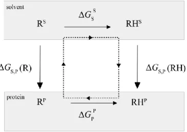
using the pKa of the model compound in solvent is based on the thermodynamic cycle shown in Figure 1.
5 1
Figure 1. Thermodynamic cycle for proton binding. RH and R represent protonated and deprotonated
2
forms of the residue, respectively, in the solvent environment as a model compound (upper) or in the 3
protein environment (lower). The superscripts are used to highlight that the polarization of residue R/RH 4
is different in the protein and solvent. With the additive force fields these polarizations are the same. 5
It is assumed that the proton binding affinity difference of a titratable residue in the protein and a model 6
compound in solvent is only due to the electrostatic interactions. For a protein containing one titratable 7
residue: 8
p𝐾aprotein= p𝐾amodel+ ∆∆𝐺/ln(10)/𝑅𝑇, [Eq 1]
9
where p𝐾amodel is the pKa of a model compound in solvent; R is the gas constant; T the temperature and
10
∆∆𝐺 is a double difference of the electrostatic free energy associated with the residue being in the protein 11
environment. It is further assumed that the electrostatic field is governed by the macroscopic Poisson (or 12
Poisson-Boltzmann) equation: 13
∇𝜀(𝑟̅)∇𝜑(𝑟̅) = −4𝜋𝜌(𝑟̅), [Eq 2] 14
where 𝜑 is the electrostatic potential, 𝜌 is the charge density and 𝜀 is the dielectric constant. This equation 15
can be numerically solved, for example on a cubic lattice by finite difference methods, to give the charging 16
free energy, 𝑊, of a set of protein atomic charges: 17 𝑊 =1 2∑ 𝑄𝑖 𝑃𝜑(𝑟̅ 𝑖) 𝑖 , [Eq 3] 18
where the summation is done over the protein atomic charges, 𝑄𝑖𝑃; 𝜑(𝑟̅𝑖) is the electrostatic potential that
19
satisfies Equation 2 and computed at the position 𝑟̅𝑖 of the atomic charge 𝑄𝑖𝑃.
20
For a macromolecule containing more than one titratable site, the protonation state of a residue, 𝜇, 21
is affected by the charge state of all other titratable residues. In this case, the fraction of molecules, 𝜃𝜇,
6
protonated at site µ at a particular pH value is given by the Boltzmann average of all microstates where this 1
residue is protonated: 2
〈𝜃𝜇〉 = (∑{𝑥̅}𝑥𝑖,𝜇exp(−∆𝐺(𝑥̅ , pH)/𝑅𝑇)𝑖 )/(∑{𝑥̅}exp (−∆𝐺(𝑥̅ , pH)/𝑅𝑇)𝑖 ), [Eq 4]
3
where the summation is done over all possible protonation microstates {𝑥̅}; 𝑥̅𝑖is a vector that defines
4
protonation microstate i; 𝑥𝑖,𝜇 is a 𝜇-th element of the vector 𝑥̅ and is 1 or 0 if residue 𝜇 is protonated or 𝑖
5
deprotonated, respectively, in the microstate i; ∆𝐺(𝑥̅ , pH) is the relative free energy of protonation of 𝑖
6
microstate 𝑥̅ , and within the context of additive force fields can be expressed as follows: 𝑖
7
∆𝐺(𝑥̅ , pH) = 𝐸(𝑥𝑖 ̅ , pH ) + ∑ (∆𝐺𝑖 𝜇 Born,𝜇(𝑥𝑖,𝜇) + ∆𝐺back,𝜇(𝑥𝑖,𝜇))+ 1
2∑𝜇≠𝜈𝑊𝜇𝜈(𝑥𝑖,𝜇, 𝑥𝑖,𝜈), [Eq 5]
8
where ∆𝐺𝐵𝑜𝑟𝑛,𝜇 is the relative Born energy of a titratable residue located in the protein environment and
9
related to its desolvation electrostatic free energy; ∆𝐺back,𝜇 is due to interactions with the background
10
charges on non-titratable residues; 𝑊𝜇𝜈(𝑥𝑖,𝜇, 𝑥𝑖,𝜈) is electrostatic interaction energy between two titratable
11
residues µ and ν being in protonation states 𝑥𝑖,𝜇 and 𝑥𝑖,𝜈 respectively. 𝐸(𝑥̅ , pH ) is a contribution from 𝑖
12
solvent pH and reference model compounds: 13
𝐸(𝑥̅ , pH) = ∑ 𝐸(𝑥𝑖 𝜇 𝑖,𝜇, pH)= ∑ (𝑥𝜇 𝑖,𝜇 𝑅𝑇 ln(10) (pH − pK𝑎,𝜇model) − 〈𝐸𝜇model(𝑥𝑖,𝜇)〉) , [Eq 6]
14
where 〈𝐸𝜇model(𝑥𝑖,𝜇)〉 is the average electrostatic free energy of the reference model compound for residue
15
𝜇 being in protonation form 𝑥𝑖,𝜇 in solvent computed using the same force field model. For the convention,
16
in summations we will use letters from the Latin alphabet to designate protein particles (atoms, Drudes, 17
lone-pairs) and protein microstates, while Greek letters to denote residues in the protein. The 〈𝜃𝜇〉 are
18
evaluated at a discrete number of pH values to obtain a titration curve for site µ. p𝐾a,𝜇 of a titratable residue
19
µ in the protein is then defined as the pH value where the titratable residue is half-protonated.
20
In practice calculations of titration curves directly using Equation 4 are limited to macromolecules 21
containing only a few titratable residues since it requires sampling of a large number of protonation 22
microstates that grows exponentially (2N) with the number of titratable residues. To solve this problem MC 23
simulations are performed to sample only relevant protonation states, while high-energy states that do not 24
contribute significantly in Equation 4 are not visited. To perform MC simulations, energies appearing in 25
Equation 5 must be precomputed and stored in the first step. Relative free energy of the protein in a 26
particular protonation state is then recovered from the energy matrices as a simple sum of energy terms in 27
the MC simulations. 28
7
The Poisson-Boltzmann method for pKa calculations with a polarizable force field and multiple
1
titratable sites
2
In the case of polarizable force fields, ∆𝐺Born,𝜇, ∆𝐺back,𝜇 and 𝑊𝜇𝜈 in Equation 5 depend on the
3
electronic state, or polarization, of all protein atoms. In particular, with the Drude force field ∆𝐺𝐵𝑜𝑟𝑛,𝜇,
4
∆𝐺back,𝜇 and 𝑊𝜇𝜈 are functions of the position of the Drudes on all atoms including titratable residues. In
5
turn, the positions of all Drudes, including on protein backbone atoms, depend on the protonation states of 6
all residues. In the case of polarizable force fields the relative free energy ∆𝐺(𝑥̅, pH) contains additional 7
contributions. In the context of the additive force field, these contributions do not depend on the protein 8
protonation state 𝑥̅, and thus do not contribute in Equation 5. These energy terms include (i) a contribution 9
from interactions between background charges with background charges, since polarization of background 10
atoms depends on the protonation state; (ii) the Born energy of background atoms, which now depends on 11
the polarization affected by the protonation state of all residues; and (iii) the polarization work needed to 12
polarize titratable and non-titratable groups of atoms from the polarization in solvent to the polarization in 13
a protein. We will use 𝐺BB(𝑥̅) to denote the sum of the first two terms (i) and (ii), and the term (iii) will be
14
included in 𝐺BB(𝑥̅), 𝐺Born,𝜇(𝑥̅), and 𝐺back,𝜇(𝑥̅). The term (iii) is computed within the Drude force field as
15
the bond energy contributed by the atomic core-Drude particle bonds (i.e. self-polarization energy term or 16
polarization work), which is different due to the different polarization in solvent and protein as well as 17
being coupled to the protein protonation state. Thus, the total relative free energy of a microstate within the 18
Drude polarizable force field is calculated using the following formula: 19 ∆𝐺(𝑥̅, pH) = 𝐸(𝑥̅, pH) + ∆𝐺BB(𝑥̅) + ∑ (∆𝐺𝜇 Born,𝜇(𝑥𝜇, 𝑥̅) + ∆𝐺back,𝜇(𝑥𝜇, 𝑥̅))+ 1 2∑𝜇≠𝜈𝑊𝜇𝜈(𝑥𝜇, 𝑥𝜈, 𝑥̅), 20 [Eq 7] 21
where 𝑥̅ is, as above, a vector with element 𝑥𝜇 defining the protonation state of residue µ; and the argument
22
𝑥̅ in functions 𝐺Born,𝜇(𝑥𝜇, 𝑥̅), 𝐺back,𝜇(𝑥𝜇, 𝑥̅) and 𝑊𝜇𝜈(𝑥𝜇, 𝑥𝜈, 𝑥̅) is repeated to emphasize that in contrast
23
to Equation 5, these terms depend on the protonation state of all residues including titratable residues µ and 24
ν.
25
In contrast to additive force fields, 𝐺(𝑥̅, pH) given by Equation 7 is not a residue-pairwise function. 26
This means that the free energy of all protein protonation microstates cannot readily be recovered in MC 27
simulations. Accordingly, in what follows, we present an approximate MC method suitable for the 28
polarizable Drude force field in the context of a constant pH formalism. We first note that to define p𝐾a,1/2
29
of a titratable residue only the point on the titration curve where pH = p𝐾a,1/2 needs to be identified. Thus,
30
the approach just needs to reproduce exactly the free energies of microstates highly populated at 31
8
pH~ p𝐾a,1/2 that contribute significantly in Equation 4. In the method presented later in this section, free
1
energies of the most populated states for the protonated and deprotonated forms of a residue are computed 2
exactly using minimization of the position of the Drudes particles (i.e. performing the polarization SCF 3
calculation) in the field of the implicit solvent. Thus, polarization effects for the most populated microstates 4
are taken into account exactly, while free energies of less populated microstates perturbed by the 5
polarization response to the change of the protonation state are computed less accurately during the MC 6
simulation. To calculate ∆𝐺BB(𝑥̅), ∆𝐺Born,𝜇(𝑥𝜇, 𝑥̅), ∆𝐺back,𝜇(𝑥𝜇, 𝑥̅) and 𝑊𝜇𝜈(𝑥𝜇, 𝑥𝜈, 𝑥̅) in Equation 7 the
7
position of all Drude particles should be defined. In the method, the highly populated protonation states at 8
pH = p𝐾a,𝜇 are used to calculate these energies for the protonated and deprotonated forms of residue µ.
9
pKa calculations with the Drude force field and Poisson-Boltzmann model
10
In this section the calculation protocol of the new method is given. A flow chart of the computational 11
protocol is presented in Scheme 1. Protonation states for all residues are predefined in the initial calculation 12
of energy terms appearing in Equation 7, with titratable residues assigned neutral protonation states. These 13
predefined states will be refined iteratively in subsequent steps. The method starts with molecular 14
mechanics (MM) and Poisson-Boltzmann calculations of free energies needed to perform MC simulations: 15
Step 1. Calculate protein free energies for both ionization states of all titratable residue with the 16
remaining titratable residues assigned neutral protonation states. For each protonation state of titratable 17
residue µ, neutral protonation states are used for all other titratable residues giving the vector defining the 18
protonation microstate 𝑥̅𝑖. These protonation microstates 𝑥̅𝑖 are used to optimize the Drude particles. The
19
free energies of the protein in each of these protonation microstates is calculated as 𝐺𝑖 = 𝐺(𝑥̅𝑖), based on
20
the system MM energy and the PB implicit solvation energy, with these energies including the polarization 21
energy following the Drude SCF calculation. 22
Step 2. Interaction free energies between titratable residues, which include MM electrostatic 23
interactions and the solvent contribution, are calculated. This involves individually calculating the 24
electrostatic potential for each titratable residue 𝜇, by zeroing the charges on all atoms in the protein 25
(including lone pairs and Drude particles) except those on the residue 𝜇. The positions of Drude particles 26
optimized in step 1 and corresponding to selected protein protonation microstates for residues 𝜇 and ν are 27
used, so no optimization of Drude particles is needed at this step. To avoid the problem of artificial 28
contributions arising when interaction energies are computed between neighboring residues due to 1,2 and 29
1,3 dipole-dipole interactions included in the Drude model, the contribution to the interaction energy from 30
solvent is computed using the PB model and combined with the MM energy to obtain the total interaction 31
free energy between residues. The PB equation is solved to obtain the electrostatic potential 𝜑𝑅𝜇(𝜀𝑒𝑥𝑡 =
9
𝜀𝑤, 𝜀𝑖𝑛𝑡 = 𝜀𝑝), due to the charges of residue 𝜇 being in the protonation state 𝑥𝜇. Calculations are repeated
1
using the protein dielectric constant for the protein exterior to obtain the electrostatic potential 𝜑𝑅𝜇(𝜀𝑒𝑥𝑡 =
2
𝜀𝑝, 𝜀𝑖𝑛𝑡 = 𝜀𝑝). The electrostatic potential is used to calculate the electrostatic interaction 𝑊𝜇𝜈 𝑥𝜇,𝑥𝜈∗
between 3
the titratable residues µ and ν being in protonation state 𝑥𝜇 and 𝑥𝜈, respectively, according to 𝑊𝜇𝜈 𝑥𝜇,𝑥𝜈∗
= 4
1/2 ∑ 𝑞𝑖𝑗 𝑖𝑞𝑗/𝜀𝑝/𝑟𝑖𝑗+ ∑ 𝑞𝑗 𝑗(𝜑𝑅𝜇𝑗(𝜀𝑒𝑥𝑡 = 𝜀𝑤, 𝜀𝑖𝑛𝑡 = 𝜀𝑝)- 𝜑𝑅𝜇𝑗(𝜀𝑒𝑥𝑡= 𝜀𝑝, 𝜀𝑖𝑛𝑡 = 𝜀𝑝)), where 𝑞𝑖 and 𝑞𝑗
5
are charges of residues 𝜇 and ν, respectively. Note that in principle 𝑊𝜇𝜈𝑥𝜇,𝑥𝜈∗≠ 𝑊𝜈𝜇𝑥𝜈,𝑥𝜇∗, and these 6
interaction energies are different from those appearing in Equation 7 since the polarization used for residues 7
µ and ν corresponds to different protein protonation microstates. We use an asterisk to distinguish these
8
energies from the interaction energies in Equation 7. 9
Step 3. For each free energy, 𝐺𝑖 computed in step 1 it is possible to write Equation 7 as follows:
10
𝐺𝑖 = 𝐺BB(𝑥̅𝑖) + ∑ (∆𝐺𝜇 Born,𝜇(𝑥𝑖,𝜇, 𝑥̅𝑖) + ∆𝐺back,𝜇(𝑥𝑖,𝜇, 𝑥̅𝑖))+ 1
2∑𝜇≠𝜈𝑊𝜇𝜈(𝑥𝑖,𝜇, 𝑥𝑖,𝜈, 𝑥̅𝑖) , [Eq. 8]
11
The latter expression does not form a closed system of linear equations relative to the terms 12
∆𝐺Born/back,𝜇(𝑥𝑖,𝜇, 𝑥̅𝑖) = ∆𝐺Born,𝜇(𝑥𝑖,𝜇, 𝑥̅𝑖) + ∆𝐺back,𝜇(𝑥𝑖,𝜇, 𝑥̅𝑖), since the latter terms are different for
13
different protonation microstates 𝑥̅𝑖. To recover 𝐺𝑖 later in MC simulations, instead of using Equation 8 we
14
introduce a system of linear equations: 15 ∑ 𝐺Born/back,𝜇𝑥𝜇1 𝜇 + 𝐺BB= 𝐺1− 1 2∑ 𝑊𝜇𝜈 𝑥𝜇1,𝑥𝜈1∗ 𝜇≠𝜈 16 ∑ 𝐺Born/back,𝜇𝑥𝜇2 𝜇 + 𝐺BB= 𝐺2− 1 2∑ 𝑊𝜇𝜈 𝑥𝜇2,𝑥 𝜈2∗ 𝜇≠𝜈 18 … [Eq 9] 17
where 𝐺BB is again due to interactions between background atoms with themselves, but invariant relative
19
to the protonation state of titratable residues; 𝑊𝜇𝜈𝑥𝜇1,𝑥𝜈1∗is the interaction energy between residues 𝜇 and 𝜈 20
computed in step 2; 𝐺Born/back,𝜇𝑥𝜇𝑖 and 𝐺BB can be regarded as unknowns that satisfy the system of equations.
21
The right hand expressions in the system are calculated in steps 1 and 2. The system of linear equations can 22
be resolved to find all 𝐺Born/back,𝜇𝑥𝜇𝑖 and 𝐺
BB.
23
We note that 𝐺Born/back,𝜇𝑥𝜇𝑖 are not calculated directly in step 1 as was performed in the original constant-24
pH MC method. This is due to the need to calculate free energies from step 1 in the MC simulations as 25
10
required to identify the most likely protonation microstates for each titratable residue as a function of pH 1
when residues titrate (at pH = p𝐾a,𝜇) rather than 𝐺Born/back,𝜇 𝑥𝜇𝑖
energies. In other words, G1, G2 … Gn are
2
used in MC simulations to sample probabilities of protonated and deprotonated states and, thus are required 3
to calculate the titration curves. It should be emphasized that in MC simulations with the Drude force field 4
it is prohibitively expensive to calculate the free energies of all protein microstates in contrast to the 5
calculations with additive force fields; instead, we recover free energies of the most important states using 6
the above method. 7
It may happen that the most likely protein microstates are identical for protonation states of different 8
residues at the pH where they are half-protonated. In this case, equations for the protonation states of these 9
residues are identical in the system of equations 9, and the system is not complete as required to define 10
𝐺Born/back,𝜇𝑥𝜇𝑖
and 𝐺BB. To complete the system we introduce additional equations in the free energy Gl
11
computed with zero charges on all titratable residues except residue µ. The additional equation added to the 12
system of equations 9 is: 𝐺Born/back,𝜇𝑥𝜇1 + 𝐺
BB= 𝐺𝑙.
13
Step 4. Perform MC simulations. During the MC simulations at the pH corresponding to the p𝐾a,𝜗 of
14
residue θ, the free energy of microstates is computed according to: 15 𝐺(𝑥̅) = 𝐺BB+ ∑ 𝐺Born/back,𝜇 𝑥𝜇 𝜇 + 1 2∑ 𝑊𝜇𝜈 𝑥𝜇,𝑥𝜈∗ 𝜇≠𝜈 [Eq. 10] 16
In Equation 10, 𝑊𝜇𝜈𝑥𝜇,𝑥𝜈∗ are the same energies used in the system of equations 9 and 𝐺
Born/back,𝜇 𝑥𝜇
and 𝐺BB
17
are the solutions. For the most populated microstate 𝑥̅𝑖, selected in Step 1, this equation should give exactly
18
𝐺𝑖. Thus, this approximation allows the free energies to be recovered in the MC simulations computed with
19
the correct polarization (e.g. SCF Drudes). It should be noted that 𝐺BB is a constant for all microstates and
20
thus, cancels out when relative free energies of microstates are computed in the MC simulations. The 21
dependence of 𝐺BB(𝑥̅) on the protonation state does not appear in Equation 10 explicitly. However, for the
22
most populated states it is included in 𝐺Born/back,𝜇𝑥𝜇
, as they are solutions of the system of equations 9. 23
MC simulations are performed in the range of pH values between -10 to 30 with a step of 0.5 pH unit 24
to obtain a titration curve for each titratable residue. The contribution 𝐸(𝑥̅, pH) computed by Equation 6 is 25
added to Equation 10 to obtain relative free energies of protein microstates. During the MC simulations one 26
randomly selected titratable residue protonation state is changed with acceptance or rejection of that change 27
based on the Metropolis criteria. In 50% of the MC steps a second residue is allowed to change its 28
protonation state. In the present study, 100,000 MC steps were performed for each titratable residue in the 29
11
system (eg. with 20 titratable residues 2·106 MC steps are performed). To test the convergence of MC
1
simulations the number of MC steps was doubled, but the change in relative populations of protonated and 2
deprotonated forms was less than 10-3 observed for residues in eight proteins. Finally, using the titration
3
curves the set of p𝐾a,𝜇 values of all titratable residues can be defined based on the pH at which they are
4
half-protonated. 5
Step 5. MC simulations for each titratable residue µ and each of its protonation state 𝑥𝜇 are repeated at
6
pH = p𝐾a,𝜇 determined in the previous step. In contrast to the MC simulations in step 4, the targeted
7
titratable residue µ is fixed in the protonation state 𝑥𝜇 to find the most likely protonation states for all other
8
titratable residues. Note that the most likely protonation states may be different for the protonated and 9
deprotonated forms of the same residue µ. The same number of MC steps was performed as in step 4. 10
Step 6. Steps 1-5 are repeated with the most likely states of each titratable residue obtained from step 11
5. These iterations are required since initially in step 1 the most likely protonation states are not known but 12
rather estimated based the neutral protonation state. Iterations over steps 1-5 are performed until the 13
calculated p𝐾a,𝜇 of all the titratable residues and the states computed in step 5 converge. Overall, the
14
protocol has two types of self-consistent iterations: (i) in step 1 the position of the Drudes and the PB 15
solvent polarization are fully optimized and (ii) globally, steps 1-6 are repeated to converge the individual 16
titratable residue p𝐾a,𝜇 values.
17 18
12
Scheme 1. Flow Chart of the computations performed with the Drude-PB method. Steps 1-5 are repeated until p𝐾a,𝜇
1
and microstates converge. Initial microstates are updated using the computed microstates at the end of the previous
2
iteration.
3
To summarize, using this method the polarization effects are included without any approximation in 4
free energies for the most populated protonation microstates of a protein when residues titrate (at pH = 5
p𝐾a,𝜇). Within this method, it is achieved at an additional computational cost to perform multiple iterations.
6
It should be noted that polarization of less populated states is still incorrectly treated, since a surrogate of 7
𝐺Born/back,𝜇𝑥𝜇 and 𝑊𝜇𝜈𝑥𝜇,𝑥𝜈∗ corresponding to protonation states that differ from that of the less populated 8
states is used. The latter error is expected to be small, since those microstates make small contributions to 9
the titration curves at pH equal p𝐾a,𝜇. Notice, that in principle, one could consider exact free energies for a
10
limited number of less occupied microstates in Equation 4, however, in this work we limit to one state per 11
protonation and rotameric state of a residue. 12
Proton binding sites and protein structure relaxation
13
In the present study, only titratable protons are allowed to change their positions to preserve the 14
dielectric boundary. Otherwise, the PB equation would need to be solved for each 𝑊𝜇𝜈 element, which is
15
prohibitively expensive. It should be noted that different approximations have been proposed with the 16
sacrifice of the exact protein boundary to allow limited flexibility of sidechains8a, 14, which will be explored
17
in future studies with the Drude force field. 18
In the case of the acidic aspartate and glutamate residues, we consider five protonation states: one 19
ionized negative state and four neutral states with the proton on either oxygen and in the syn and anti 20
orientations. Two rotamers were included for neutral tyrosine that differ by the orientation of the hydroxyl 21
group, and three rotamers for the neutral lysine, distinguished by the dissociation of amino protons. 22
Histidines had two possible neutral tautomers: protonated on Nε (pKa of the model compound 7.0) and Nδ
23
(pKa of the model compound 6.5). In the implementation, the neutral tautomers of histidines are simply
24
treated as "rotamers" with a different contribution to the pH dependent term due to the pKa difference of
25
the Nε and Nδ sites. The total number of rotamers for neutral and ionized forms for titratable residues was 26
chosen to be identical to avoid the problem of artificial biasing in MC simulations of protonation forms 27
having a larger number of rotamers. 28
Reference state
29
Following the thermodynamic cycle shown in Figure 1, to calculate the protonation free energy in 30
the protein the free energy of the model compound in solution, called the reference free energy, is 31
subtracted. This free energy is estimated using the same force field model, which is needed for the 32
cancelation of artefacts due to the employment of the empirical force field model. The force field term of 33
13
the reference free energy is estimated as the free energy of the model compound in solution averaged over 1
all possible compound conformations. In this work, we neglect the contribution from the bonded terms not 2
associated with the Drude particles, since a single conformation for the protein calculations is used. Thus, 3
the reference free energy of a model compound with a titratable residue x in solvent is: 4
𝐺𝑥ref= 𝐸elec+ 𝐸bondDrude+ 𝐺solvPB , [Eq 11]
5
where 𝐸𝑒𝑙𝑒𝑐 is the intramolecular electrostatic energy computed with the same dielectric constant 𝜀𝑝, which
6
is used to calculate the solvation free energy
7
𝐺solvPB = 𝐺𝜀𝑒𝑥𝑡=80PB − 𝐺𝜀𝑒𝑥𝑡=𝜀𝑝
PB . The same dielectric constant is also used for the protein calculations. 𝐸 bondDrude
8
is the bond energy from the atomic core-Drude particle bonds (i.e. self-polarization energy term or 9
polarization work).15N-acetyl-x-N-methylamide with the corresponding titratable residue x was used as the
10
model compound in solution. In this compound, charges involved in all 1-4 electrostatic interactions, 11
including Drudes are identical to those charges in the protein system, leading to the cancelation of artefacts 12
arising from the employment of the force field. To obtain pKa 's in the protein, the computed pKa shifts due
13
to the protein environment were added to p𝐾amodel's given in Table S2. The experimental pKa shifts were
14
computed as the difference between the pKa in the protein environment and the pKa of the corresponding
15
model compound. 16
To obtain average free energies in solvent we performed molecular dynamics (MD) simulations of 17
the N-acetyl-x-N-methylamides immersed in a cubic solvent box. The minimum distance between the
18
compound atoms and the edge of the system was 12 Å. Periodic boundary conditions were assumed. All 19
long range electrostatic interactions were computed efficiently by the particle mesh Ewald method16 using
20
a real space cutoff of 12 Å. The Lennard-Jones term was evaluated out to 12 Å with a force switch 21
smoothing function from 10 to 12 Å. MD simulations were performed at a constant temperature of 298 K 22
and pressure of 1 ATM after 20 ps of thermalization. During MD simulations the center of mass of the 23
model compound atoms was weakly harmonically restrained to the origin of the system with a force 24
constant of 1.0 kcal·mol-1·Å-2. For the model compounds the CHARMM36 (C36)17 and Drude18 protein
25
force fields were used along with the CHARMM TIP3P19 and SWM4-NDP20 model for water for the
26
additive and polarizable calculations, respectively. Simulations were done with the NAMD program.21 50
27
nanoseconds of MD were performed at constant temperature and pressure for the compound containing 28
each titratable residues. To calculate PB free energies, structures from the MD simulations were saved every 29
100 ps. The final PB free energies were averaged over these structures. The convergence was confirmed by 30
dividing the data into five blocks corresponding to 10 ns MD simulations and computing the standard 31
deviation, which was lower than 0.1 kcal·mol-1 in all cases.
14
For the protonated form of the carboxylic acids, Asp and Glu, the syn and anti positions of the OH 1
proton were simulated separately. The reference energy of the protonated form of Asp and Glu was 2
Boltzmann-averaged over the free energies of the two forms. 3
Internal dielectric constant
4
As demonstrated and discussed in the work of Warshel et al, the dielectric constant ascribed to the 5
protein medium is meant to represent physical contributions that are not considered explicitly.22 In the early
6
model of Tanford and Roxby a protein was treated as a medium with a dielectric constant 𝜀𝑖𝑛𝑡 = 4 and
7
solvent with a dielectric constant of 80, the experimental value. The protein dielectric constant of 4 is larger 8
than the electronic polarizability estimate of 2, presumably to take into account the contribution due to the 9
fluctuations of protein polar groups about their equilibrium positions.9, 23 In the model of Tanford and
10
Roxby, the uniform continuum medium representing the interior of the protein, itself treated as a fixed 11
object, was meant to implicitly incorporate the effects of the atomic fluctuations. This model is clearly an 12
approximation. Obviously, the choice of the dielectric constant ascribed to the protein interior depends on 13
the physical effects that are treated explicitly in the model.10a, 24 In this work, we do not treat fluctuations of
14
protein atoms explicitly, which justifies the use of a higher dielectric constant for the protein interior (𝜀𝑖𝑛𝑡 >
15
1). However, since reorganizations in the protein electronic structure are treated explicitly in the polarizable 16
model, the protein dielectric constant is expected to be smaller than in the model with the additive force 17
field. This conjecture will be verified with practical examples below. Following our previous work, the 18
ionic strength was set to 0 M.15
19
Poisson-Boltzmann free energy calculations with the Drude Force field
20
The Poisson-Boltzmann free energy with the Drude force field is calculated in accord with our
21
previous work.15 In brief, we need to calculate the electrostatic free energy, 𝐺
𝜀𝑒𝑥𝑡=𝜀𝑤,𝜀𝑖𝑛𝑡=𝜀𝑝 of a solute with 22
an internal dielectric constant of 𝜀𝑝immersed in a dielectric medium with a high dielectric constant of 𝜀𝑤.
23
The free energies computed using the potential obtained by numerically solving the Poisson-Boltzmann 24
equation and Equation 3 contain the artificial contributions of the grid as well as from electrostatic 25
interactions between 1-2 and 1-3 bonded atoms. These contributions in the PB model should be removed 26
by subtraction. To correct the electrostatic component of the free energy we modify 𝐺𝜀𝑒𝑥𝑡=𝜀𝑤,𝜀𝑖𝑛𝑡=𝜀𝑝 by the 27
free energy computed with a uniform dielectric constant of 𝜀𝑝:
28
𝐺𝜀𝑒𝑥𝑡=𝜀𝑤,𝜀𝑖𝑛𝑡=𝜀𝑝= 𝐺𝜀𝑒𝑥𝑡=𝜀𝑤,𝜀𝑖𝑛𝑡=𝜀𝑝− 𝐺𝜀𝑒𝑥𝑡=𝜀𝑝,𝜀𝑖𝑛𝑡=𝜀𝑝+ 𝐺𝜀𝑒𝑥𝑡=𝜀𝑝,𝜀𝑖𝑛𝑡=𝜀𝑝, [Eq 12] 29
where 𝐺𝜀𝑒𝑥𝑡=𝜀𝑝,𝜀𝑖𝑛𝑡=𝜀𝑝 is the contribution from the solute-solute interactions in a uniform dielectric medium 30
with a dielectric constant of 𝜀𝑝 and is computed using 𝐺𝜀𝑒𝑥𝑡=𝜀𝑝,𝜀𝑖𝑛𝑡=𝜀𝑝=
1 2∑
𝑞𝑖𝑞𝑗
𝜀𝑝𝑟𝑖𝑗
𝑖≠𝑗 . The first two terms
15
are computed using the Poisson-Boltzmann equation using the same set of parameters including those that 1
define the grid, except the external dielectric constant. In this case, the artificial contributions cancel out, 2
since the internal dielectric constant in both calculations is the same. In these calculations the state with the 3
uniform dielectric constant, 𝜀𝑝, is used as a reference state. To obtain the total free energy of a solute, the
4
electrostatic component given by Equation 12 should be supplemented by self-polarization work, which is 5
computed within the Drude force field as the bond energy contributed by the atomic core-Drude particle 6
bonds. 7
An additional complication with a polarizable force field is that the interaction energy 8
𝑊𝜇𝜈(𝑥𝑖,𝜇, 𝑥𝑖,𝜈) in Equation 7 includes the electronic energy of the entire system that includes the
self-9
polarization energy and the 1-2, 1-3 contributions from Drude particles. These terms disallow the 10
calculation of 𝑊𝜇𝜈(𝑥𝑖,𝜇, 𝑥𝑖,𝜈) for two neighboring residues using only the Poisson-Boltzmann model. This
11
is not the case for additive force fields where charges on the backbone atoms are normally fixed to the same 12
values in the protonated and deprotonated forms, and thus these contributions cancel out for neighboring 13
residues when the protonation free energy is computed. Thus, for the Drude force field the combination of 14
the MM energy and PB solvation free energy are used to calculate the interaction energy, 𝑊𝜇𝜈(𝑥𝑖,𝜇, 𝑥𝑖,𝜈),
15
as described above. 16
We use the solvation radii that were optimized in our previous work to reproduce experimental
17
solvation free energies of a set of small molecules.15 The solvation radii were defined for all atom types
18
except the deprotonated hydroxyl oxygen in tyrosine. The missing solvation radius of the O- oxygen was
19
optimized to reproduce the experimental absolute solvation free energy of the deprotonated tyrosine as 20
described in the Supplementary Information. 21
PB free energy calculations were performed with the PBEQ module25 implemented in the CHARMM
22
program.26 To include polarization effects explicitly the positions of Drude particles were optimized with
23
the nuclear positions constrained in each protein microstate in step 1 using 50 steps of the Steepest Descent 24
minimizer. Previously we showed that 20 steps of optimization was adequate for the minimization 25
convergence for a set of protein complexes.15 As previously, dummy atoms were added to fill internal
26
cavities not accessible by water molecules with a low dielectric medium.15 The protein PB energies were
27
computed using the focusing method with a coarse grid of 0.8 Å resolution and fine grid with 0.4 Å 28
resolution. The ion concentration was set to zero; we continue to call this method PB for the sake of 29
simplicity, but use the finite-difference Poisson equation with no electrolyte present in the continuum 30
solvent. The program to perform Monte-Carlo simulation for pKa calculations was written in C++. The
31
system of linear equation 9 was solved using the Eigen library for linear algebra.27
16
Protein data set for pKa calculations
1
The data set includes 94 titratable residues from eight proteins (Table S1, Supporting information). 2
Protein structures were retrieved from the Protein Data Bank (PDB) and used for the position of heavy 3
atoms in all calculations. Hydrogens were built using CHARMM,26 and optimized with a uniform dielectric
4
constant of 4 and titratable residues set to the standard protonation states at pH 6.5 (carboxylic acids 5
deprotonated; lysines and tyrosines protonated; histidines doubly protonated). In this work we consider 6
Asp, Glu, His, Lys, and Tyr as titratable, while Arg residues were present only in the protonated form. The 7
protein data set did not contain any titratable cysteines. The N- and C-termini were not considered as 8
titratable and were fixed in the standard protonation state, i.e. the terminal amino group is protonated and 9
terminal carboxylate group is deprotonated. Thus, the data set included 31 aspartic acids, 30 glutamic acids, 10
10 tyrosines, 17 lysines and 6 histidines. Most of the experimental pKa values used in this study were
11
compiled by Georgescu et al.14 The experimental pK
a's for the SNase variant Δ+PHS were taken from
12
Castaneda et al.3
13
RESULTS
14
Polarization effect on interaction free energies between titratable residues
15
We first examine the effect of polarization due to protonation of protein titratable sites on 16
interaction free energies, 𝑊𝜇𝜈𝑥𝜇,𝑥𝜈 to test the approximation that these terms do not change significantly in 17
the polarizable force field. Within classical additive force fields 𝑊𝜇𝜈𝑥𝜇,𝑥𝜈 are independent of protonation 18
states of all residues except the protonation state 𝑥𝜇 and 𝑥𝜈 of the corresponding pair of residues 𝜇 and 𝜈.
19
With polarizable force fields, in principle 𝑊𝜇𝜈𝑥𝜇,𝑥𝜈 depends on the protonation state of all protein titratable 20
sites: 𝑊𝜇𝜈𝑥𝜇,𝑥𝜈 = 𝑊
𝜇𝜈 𝑥𝜇,𝑥𝜈
(𝑥̅). To estimate the magnitude of this dependence we computed 𝑊𝜇𝜈𝑥𝜇,𝑥𝜈 for 21
different pairs 𝜇 and 𝜈 in the eight proteins from the data set and random protein protonation states as 22
follows. Random protonation states for each of the proteins were generated with the number of the 23
generated random protonation states proportional to the number of titratable residues. The positions of the 24
Drude particles were then fully optimized for each of these protonation states using the PB implicit solvent 25
model for the complete protein structures. For these calculations, the dielectric constant of two was used 26
for the protein interior. The interaction free energies, 𝑊𝜇𝜈𝑥𝜇,𝑥𝜈
, were then calculated yielding around 20 27
values for each 𝑊𝜇𝜈𝑥𝜇,𝑥𝜈 interaction energy when all the randomly generated models were considered. These 28
interaction free energies for a pair of residues are different due to the protonation states of other residues 29
through induced polarization. Table 1 gives statistics of computed interactions. The average absolute 30
difference in the interaction free energy over all pairs of titratable residues is just 5·10-4 kcal·mol-1 for the
17
protein 1a2p, and values of a similar magnitude were found for the other proteins in the data set. The 1
maximum absolute difference in 𝑊𝜇𝜈𝑥𝜇,𝑥𝜈
due to the protein protonation state is less than or equal to 0.15 2
kcal·mol-1 for all protein except SNase variant Δ+PHS (PDB reference code 3bdc) and ribonuclease A
3
(PDB reference code 3rn3). In SNase the large effect on the interaction is observed for the pair Tyr91-4
Glu75. This is explained by the fact that these residues directly interact with other titratable residues: Tyr91 5
makes a hydrogen bond with Asp77, and Glu 75 interacts with Tyr93 and His121. Deprotonation of these 6
residues has a strong effect on the polarization of Tyr91 or Glu75 due to strong and unfavorable electrostatic 7
interactions. In fact, we expect this effect to be smaller if the protein flexibility is taken into account and 8
these pairs are allowed to rearrange upon titration. The maximum variation in 𝑊𝜇𝜈𝑥𝜇,𝑥𝜈 in SNase excluding 9
this pair is less than 0.1 kcal·mol-1. Overall, we find that the effect of the induced polarization on interactions
10
between ionizable residues due to the protein protonation state to be negligible for the eight proteins in the 11
data set thereby allowing this term to be calculated based on a single protonation state of the system. 12
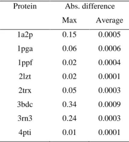
Table 1. Absolute difference in the interaction free energies due to randomly-generated variations in the
13
protein protonation state. Calculations used the protein dielectric constant of two and the Drude force 14
field. Energies are given in kcal·mol-1.
15
Protein Abs. difference
Max Average 1a2p 0.15 0.0005 1pga 0.06 0.0006 1ppf 0.02 0.0004 2lzt 0.02 0.0001 2trx 0.05 0.0003 3bdc 0.34 0.0009 3rn3 0.24 0.0003 4pti 0.01 0.0001 16
Contribution of the polarization on background atoms induced by titration
17
Next the polarization effect of background atoms due to changes in protonation state of titratable 18
residues on computed pKa's was examined. This polarization contributes directly to interactions between
19
titratable residues and background atoms, i.e. to the term 𝐺Born/back,𝜇𝑥𝜇
, as well as changes the interactions 20
of background atoms with themselves 𝐺BB(𝑥̅). To test if 𝐺BB(𝑥̅) can significantly influence the population
21
of the protonated versus deprotonated forms of a titratable residue we computed 𝐺BB(𝑥̅) with different
22
protonation states of the protein as follows. First, the most likely protein protonation state 𝑥̅ was computed 23
at the pH where a titratable residue is half protonated with a protein dielectric constant of 4. 𝐺BB(𝑥̅) were
18
then computed for all residues from the data set and all possible protonation states with the correct 1
polarization, i.e. the polarization computed in the first step presented in the Methods section. The results 2
are given in Table 2. As can be seen 𝐺BB(𝑥̅) depends on the protonation state of titratable residues only
3
moderately. For all studied proteins, the average values of 𝐺BB(𝑥̅) are close to those obtained through
4
solution of the system of equations 9. For example, for lysozyme (PDB 1a2p), the standard deviation of 5
𝐺BB(𝑥̅) due to residue protonation states is just 0.3 kcal·mol-1. Further analysis demonstrated that the largest
6
variations in 𝐺BB(𝑥̅) are associated with either interactions with arginines treated as background
non-7
titratable atoms in the present work or very unfavorable interactions with the background atoms, explained 8
by the fact that no explicit relaxation is taken into account. Thus, the results in Table 2 indicate that the 9
polarization of the background charges induced by titration can be neglected in the calculation of 𝐺BB(𝑥̅)
10
for pKa calculations thereby avoiding recalculation of this term for all protonation states.
11
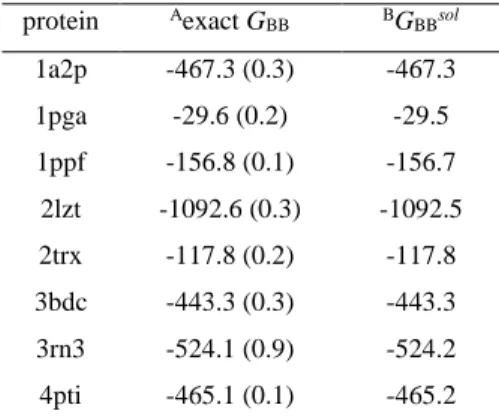
Table 2. Average contribution of background charges, 𝐺BB(𝑥̅), to the calculated total free energy
12 (kcal·mol-1). 13 protein Aexact G BB BGBBsol 1a2p -467.3 (0.3) -467.3 1pga -29.6 (0.2) -29.5 1ppf -156.8 (0.1) -156.7 2lzt -1092.6 (0.3) -1092.5 2trx -117.8 (0.2) -117.8 3bdc -443.3 (0.3) -443.3 3rn3 -524.1 (0.9) -524.2 4pti -465.1 (0.1) -465.2
AThe average value of the exact 𝐺
BB(𝑥̅) computed for the most populated protonation states for each
14
titratable residue in the proteins; standard deviations are given in parenthesis; B𝐺
BB(𝑥̅) obtained as a
15
solution to the system of equations 9. 16
pKa calculation with the Drude-PB model
17
Comparison to the exact solution
18
Initially, the method for pKa calculations with the Drude model was tested on a simple system with
19
fewer titration sites, for which the direct application of Equation 4 is still feasible. Lysozyme (PDB 20
reference code 2LZT) was chosen as a test protein. To allow the application of Equation 4 only aspartates 21
and glutamates were considered in the calculations as titratable and all other titratable residues were fixed 22
in the standard protonation state at physiological pH, i.e. lysines and tyrosines protonated. Only one syn 23
orientation for the proton in the protonated form was considered. With 7 aspartic and 2 glutamic acids, it 24
gives 512=29 possible protonation states. The structures corresponding to all possible protonation states
25
were generated, and Drude particles were fully optimized in the field of the PB implicit solvation model in 26
19
each of the structures. The internal dielectric constant of two was used. The total free energies were used 1
to compute an average number of bound protons using Equation 4. pKa's were estimated as the pH where
2
residues were half-protonated on average. pKa's were also calculated using the new method.
3
For the lysozyme system the new method converged within two self-consistent iterations as 4
computed pKa's were invariant with more iterations. The results indicate that the computed pKa's with the
5
new method and two iterations are practically identical to those estimated with the exact form of Equation 6
4. The RMS deviation between pKa's computed with the two methods is just 0.02 pH units. pKa's computed
7
with one iteration of the new method differ more from the ones computed with the exact statistical approach, 8
by 0.07 pH units. 9
pKa calculations were performed with the protein dielectric constant of 4 and the Drude-PB model
10
for all 8 proteins. The self-consistent iterations were repeated four times. The results for the pKa calculations
11
versus the experimental values as well as subsequent iterations as a function of the number of iterations are 12
given in Table 3. The RMS deviation between pKa's computed after the second iteration relative to those
13
after the first iteration is 0.15 pH units, and reduces to 0.10 and 0.08 pH units after the third and the fourth 14
iterations, respectively. However, that RMS deviation between computed and experimental pKa’s only
15
changes insignificantly from 1.94 to 1.93 pH units after the second iteration and stays practically the same 16
after the third and fourth iterations. The linear correlation between computed and experimental pKa's, R,
17
does not improve. However, the computed pKa's slightly change as a function of the number of iterations.
18
Importantly, the difference between the first and subsequent iterations is that the polarization is inconsistent 19
in the first round of pKa calculations, but it is improved in the subsequent iterations. Though we find only
20
a moderate change due to the consistent treatment of the polarization, it may be attributed, at least in part, 21
to the lack of the protein flexibility in this work. In the following sections, all results of pKa calculations
22
with the Drude-PB model will be presented using two iterations, since the computed pKa's change less than
23
0.1 pH units with more iterations and the exact pKa's were reached within two iterations for the reduced
24
lysozyme system. 25
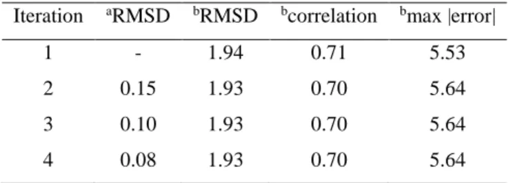
Table 3. Convergence of the pKa calculation method with the Drude-PB model. Calculations were done 26
using the protein dielectric constant of 4. 27
Iteration aRMSD bRMSD bcorrelation bmax |error|
1 - 1.94 0.71 5.53
2 0.15 1.93 0.70 5.64
3 0.10 1.93 0.70 5.64
20
aRMS deviation between pK
a's computed in this step and in the previous step; brelative to the experimental
1
pKa's
2
Comparison of the polariable Drude and additive C36 force fields.
3
To test the dependence of the result on the internal dielectric constant, pKa calculations were
4
performed with 𝜀𝑝 in the range between 1 and 20 with the Drude and C36 force fields. For the calculations
5
with the Drude force field, the resulting pKa’s were taken after the second self-consistent iteration. For the
6
calculations with C36, only one iteration is required as electronic polarization is included implicitly. The 7
results are summarized in Table 4. The computed and experimental pKa shifts are given in Table S3, and
8
absolute pKa's are given in Table S4 in the Supplementary Information. Figure 2 shows the dependence of
9
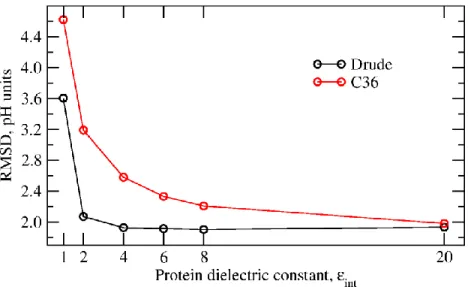
the RMS deviation against the internal dielectric constant. The correlation is best with both models at the 10
internal dielectric constant of two. However, in contrast to the results obtained with the C36 force field, 11
with the Drude model the RMS deviation is characterized by a shallow minimum at ε in the range of 4-8. 12
With the additive force field, the RMS deviation is improving monotonically in the tested range of ε. 13
Overall, the Drude model demonstrates a better agreement with the experimental pKa's than the C36 model
14
at low values of the dielectric constant. The RMS deviation between the experimental pKa's and pKa's
15
computed using the protein dielectric of two is 2.07 and 3.19 units with the Drude and C36 force fields, 16
respectively. With the protein dielectric constant of four, the RMS deviation is 1.93 and 2.58 units with the 17
Drude and C36 force field, respectively. With the Drude-PB model, the RMS deviation between the 18
experimental pKa's and pKa's computed with the protein dielectric constant of 20 is 1.93, which is very close
19
to the result of 1.93 and 2.07 units computed with the protein dielectric constant of four and two, 20
respectively. In contrast to the results with the additive C36 model, the RMS deviation computed with the 21
Drude-PB model is substantially less sensitive to the choice of the internal dielectric constant. However, 22
with the Drude model, the RMS deviation sharply increases with an internal protein dielectric constant 23
𝜀𝑝=1, and the linear correlation decreases to 0.46. A Drude-PB model with 𝜀𝑝= 1 accounts only for the
24
induced polarization, leaving out all contributions from structural fluctuations. The poor performance 25
suggests that such a model does not represent the protein interior as sufficiently polarizable. Interestingly, 26
the RMS deviation for the Drude model with 𝜀𝑝= 1 is very similar to the RMS deviation for the additive
27
force field with 𝜀𝑝≈ 1.7, a value that corresponds roughly to the expected dielectric constant associated
28
with electronic induced polarization. 29
Table 4. Performance of the methods for pKa calculations against experimental pKa‘s. RMS deviation and
30
linear correlation coefficient between computed and experimental pKa shifts from the model compound
31
reference values are given. 32
21
dielectric, εp Drude C36 Drude C36 Drude C36
1 3.57 4.62 0.46 0.71 1.8 3.6 2 2.07 3.19 0.71 0.74 1.7 2.6 4 1.93 2.58 0.70 0.73 1.5 2.0 6 1.91 2.33 0.67 0.71 1.4 1.7 8 1.90 2.21 0.64 0.68 1.3 1.5 20 1.93 1.98 0.53 0.57 1.0 1.1
AThe slope of the liner fit to the computed and experimental pK
a shifts.
1
2
Figure 2. RMS deviation between experimental and computed pKa’s. pKa’s with the Drude force field
3
were calculated using two iterations to determine the most probable protonation microstates. 4
Figure 3 gives the comparison between experimental and predicted pKa shifts with the protein
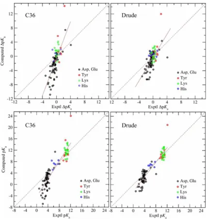
5
dielectric constant of two and the Drude and C36 models. As may be seen, with both Drude and C36 models 6
computed pKa shifts are both systematically underestimated and overestimated relative to the experimental
7
values, so that a linear fit has a constant positive slope. This slope is also given in Table 2 as a function of 8
the protein dielectric constant. However, the pKa computed with the Drude model are systematically less
9
over and underestimated in comparison with the results obtained with the C36 model. The slope with the 10
internal dielectric constant of two is 1.7 and 2.6 with the Drude and C36 models, respectively. The slope is 11
decreasing with the higher protein dielectric constant and with 𝜀int = 20 it is practically 1.0 with both
12
models. Figure 3 also contains comparison of the absolute computed and experimental pKa values. The
13
correlation coefficients for the absolute pKa’s were 0.93 and 0.91 for the Drude and C36 force fields,
14
respectively. These values are higher than those for the pKa shifts reported in Table 4 due to the wider range
15
of absolute pKa’s associated with the different classes of residues.
16 17
22 1
Figure 3. Experimental vs computed pKa shifts and absolute pKa's. Left panels: (upper) pKa shifts and
2
(lower) absolute pKa's computed with the C36 force field; right panels: (upper) pKa shifts and (lower)
3
pKa's computed with the Drude force field after iteration 2. In both calculations, the protein dielectric
4
constant of two was used. The solid line shows the linear fit to the data; the dashed line shows the perfect 5
match between computed and experimental pKa shifts or pKa's.
6
Table 5 gives the comparison between pKa shifts computed with the Drude and C36 models. With
7
the low internal dielectric constant of two, the RMS deviation between pKa shifts of the titratable residues
8
in the eight proteins computed with the two methods is 1.78 units and decreases with the higher dielectric 9
constant values. With 𝜀int= 20, the pKa shifts computed by the two methods are very close with the RMS
10
deviation of just 0.34 units. The linear correlation between pKa shifts computed by the two methods is 0.92
11
and 0.99 with 𝜀int= 2 and 𝜀int= 20, respectively. This further demonstrates that at the high internal
12
dielectric constant pKa's computed with the C36 model converge to those obtained with the polarizable
13
Drude model. This result may be understood by the fact that with the high dielectric constant, electrostatic 14
interactions are screened strongly, and thus polarization contributions due to those interactions are expected 15
to be smaller. In other words, with the high internal dielectric constant, protein polarization is close to that 16
observed in individual residues in solvent, so the difference in polarization observed in solvent and in the 17
protein plays a smaller role in pKa calculations in accordance with the thermodynamic cycle in Figure 1.
23
Table 5. Comparison between pKa shifts computed using the Drude and additive C36 models. RMS 1
deviation and linear correlation coefficient between pKa shifts computed with the Drude and C36 model
2
are given. pKa shifts computed with the Drude model were taken after two iterations in the method.
3
Protein dielectric RMSD Correlation constant, εp 2 1.78 0.92 4 0.93 0.97 6 0.68 0.98 8 0.58 0.98 20 0.34 0.99 4
The agreement between experimental and computed pKa shifts for different residue types is given
5
in Table 6. pKa's were computed using the C36 and Drude force fields and the dielectric constant of 2. For
6
all residue types, the RMS deviation with the Drude force field is better than with the additive force field. 7
The RMS deviation is 3.23 units for tyrosines with the Drude force field, which is higher than the RMS 8
deviation obtained for the other types. A similar result was obtained with the C36 force field. This may be 9
due to the need for larger conformational rearrangements of the protein to occur upon changes in the 10
protonation state of tyrosines, since they are larger than other residues and are frequently buried in the 11
protein. The poorer correlations for His and Lys with both force fields may indicate the need for larger 12
conformation changes of those sidechains upon changes in protonation. Further studies are required to 13
address these issues. 14
Table 6. Performance of the methods for pKa calculations against experimental pKa‘s for different types
15
of residues. RMS deviation and correlation coefficient between computed and experimental pKa shifts.
16
Residue N sites RMSD Correlation
Drude C36 Drude C36 Asp 31 2.10 3.40 0.66 0.78 Glu 30 2.01 3.40 0.65 0.64 His 6 1.18 1.41 0.18 0.27 Tyr 10 3.23 4.25 0.73 0.69 Lys 17 1.38 1.88 0.19 0.23 17
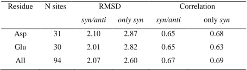
Proton orientation in the protonated form of carboxylic acids
18
The majority of constant pH studies to date have limited treatment of the orientation of the proton 19
in neutral carboxylic acids to the syn form,28 omitting consideration of the anti orientation, which is known
20
to be accessible in condensed phase environments.29 To investigate if this approximation may be limiting
21
the accuracy of the pKa estimates of acidic residues we undertook calculations of the carboxylic acid pKa