Caution, Drivers! Children Present:
Traffic, Pollution, and Infant Health
Christopher R. Knittel, Douglas L. Miller,
and Nicholas J. Sanders
CAUTION, DRIVERS! CHILDREN PRESENT: TRAFFIC, POLLUTION, AND INFANT HEALTH
Christopher R. Knittel Douglas L. Miller Nicholas J. Sanders
ABSTRACT
Since the Clean Air Act Amendments of 1990 (CAAA), atmospheric concentration of local pollutants has fallen drastically. A natural question is whether further reductions will yield additional health benefits. We further this research by addressing two related research questions: (1) what is the impact of
automobile driving (and especially congestion) on ambient air pollution levels, and (2) what is the impact of modern air pollution levels on infant health? Our setting is California (with a focus on the Central Valley and Southern California) in the years 2002-2007. Using an instrumental variables approach that exploits the relationship between traffic, ambient weather conditions, and various pollutants, our findings suggest that ambient pollution levels, specifically particulate matter, still have large impacts on weekly infant mortality rates. Our results also illustrate the importance of weather controls in measuring pollution’s impact on infant mortality.
Christopher R. Knittel Nicholas J. Sanders
MIT Sloan School of Management Stanford University
100 Main Street, E62-513 366 Galvez Street, Room 228
Cambridge, MA 02142 Stanford, CA 94305-6015
and NBER [email protected]
[email protected] Douglas L. Miller
University of California, Davis Department of Economics One Shields Avenue Davis, CA 95616-8578 and NBER
This paper has benefitted from Janet Currie, Matthew Neidell, seminar participants at UC Davis, UC San Diego, and the University of California Energy Institute, and attendants of the NBER Summer Institute and Toxic Substances Research & Teaching Program Symposium (TSR&TP). Knittel gratefully acknowledges financial support from the University of California Energy Institute and UC Davis Institute of Transportation Studies. Sanders gratefully acknowledges funding from the UC Davis Institute of Governmental Affairs, the UC Davis Institute of Transportation Studies, and the TSR&TP through the Atmospheric Aerosols and Health (AAH) Lead Campus program.
© 2011 by Christopher R. Knittel, Douglas L. Miller, and Nicholas J. Sanders. All rights reserved. Short sections of text, not to exceed two paragraphs, may be quoted without explicit permission provided that full credit, including © notice, is given to the source.
1
Introduction
Local air pollution levels have decreased dramatically over the past two decades. This is due, in large part, to the Clean Air Act and its various amendments, which placed strict limits on the con-centrations of “criteria pollutants.”1 Since 1990, the Clean Air Act Amendments of 1990 (CAAA) have helped decrease the concentration of carbon monoxide (CO) has fallen by 68 percent; ozone (O3) has decreased by 14 percent, while particulate matter 10 micrometers or smaller (PM10) has decreased by 31 percent.2 These reductions have been financially costly. The Environmental
Pro-tection Agency (EPA) estimates the compliance costs of the CAAA to be $19 billion annually in 2000, increasing to $27 billion by 2010. Over half of these costs are due to the CAAA’s National Ambient Air Quality Standards, regulating point and area sources. Regulation of mobile sources accounts for an additional 30%.3
The benefits from air quality improvements are more difficult to measure. Estimates often rely on correlations between pollution levels and health outcomes that may not reflect causal relation-ships. The EPA (1999) estimates a wide range for the potential benefits in 2000 — from a low of $16 billion to a high of $140 billion.4 This range reflects uncertainty with respect to how specific
sources affect air quality and how increasing air quality improves health outcomes. Currie and Neidell (2005) examined how California’s reductions in carbon monoxide, particulate matter, and ozone during the 1990s impacted weekly infant mortality rates, providing some evidence as to the benefits of criteria pollutant reduction. We add to the understanding of these issues by address-ing two related research questions: (1) what is the impact of automobile drivaddress-ing (and especially congestion) on the ambient air pollutants considered in Currie and Neidell (2005), and (2) what is the impact of ambient pollution on infant health in the new millennium, using local traffic varia-tion as an instrument for polluvaria-tion? In doing so, we address the potential importance of weather conditions in the estimation of pollution’s impact on health.
Our empirical strategy is as follows: when traffic is heavy, more emissions are released into the air, providing a correlation between traffic congestion and ambient pollution levels. In addition, we
1The term “criteria pollutants” refers to six commonly found air pollutants that are regulated by developing
health-based and/or environmentally-health-based criteria for allowable levels. The current criteria pollutants are: particular matter, ground-level ozone, carbon monoxide, sulfur oxides, nitrogen oxides and lead.
2Taken from http://www.epa.gov/air/airtrends/. Carbon monoxide is measured as the second highest maximum
eight hour period from 206 sites; ground-level ozone is measured as the fourth highest maximum eight hour period from 547 sites; PM10 is measured as the second highest 24 hour period average from 325 sites.
3Available at http://www.epa.gov/air/sect812/.
argue that, when regions experience unusually heavy traffic (traffic that deviates from the regional norm), such as shocks due to accidents or road closures, these shocks to traffic, and thus pollution, are likely to be uncorrelated with the error term in a model of infant mortality as a function of pollution exposure.
There are a number of reasons ordinary least squares (OLS) could yield inconsistent estimates of the impact of pollution on infant health. First, mothers may self-select into geographic regions. If mothers with higher values for clean air choose to live in cleaner areas, and these mothers are also wealthier or have access to better health care, OLS estimates may be biased upwards (e.g., Currie (2011)). In principle, including region by time fixed effects would control for this selection. However, the researcher must choose a coarser set of time fixed effects than the periodicity of the pollution data, leaving room for selection within the time fixed effects. Second, changes in local economic activity may be correlated with both pollution and infant health. Regional growth will tend to increase pollution levels, but may also be correlated with increases in income levels and/or health care access. This would tend to bias the OLS estimate downward. Third, pollution assignment leads to potential bias in the form of measurement error. The majority of papers in the air pollution and health literature, including this one, assign pollution levels to a particular person, living in a particular geographic area (e.g., zip code or county), based on pollution readings from pollution sensors in or near this geographic area. The researcher may not know the person’s exact residence (two recent exceptions to this limitation are Currie et al. (2009b) and Currie and Walker (2011)), and it is unlikely that the person is stationary over the time period analyzed. In addition, unless the exact model of spatial dispersion of the pollutant is known, even if the person lived in the assigned location and never moved from this space, pollution would be measured with error. Insofar as this measurement error is “classical” OLS estimates will be biased downward. If the measurement error is correlated with pollution levels, then the bias may be in either direction.
An additional concern is that individuals engage in avoidance behavior when confronted with bad air quality days, which will also bias OLS results toward zero. Neidell (2009) show that attendance drops on spare the air days, and that this drives OLS estimates of the impact of ozone on asthma hospitalizations, and Moretti and Neidell (2011) perform instrumental variables estimates of ozone’s impact on hospitalizations, using timing of Port of Los Angeles traffic and distance to the port as an instrument for ozone. They find IV results that are much larger than those obtained by OLS, suggesting the presence of avoidance behavior. Similarly, Graff Zivin and Neidell (2009) show people reallocate activities across time when faced with bad air quality days.5
pollu-Shocks to traffic are a potential instrument for all three sources of bias. If people sort them-selves based on average levels of pollution and traffic, but not shocks or the likelihood of shocks, then our instrument strategy will satisfy the exclusion restriction; similarly, weekly variation in traffic shocks (after conditioning on geographic and time fixed effects) are also more likely to be uncorrelated with economic growth.6 In addition, an instrumental variables approach is a stan-dard solution for measurement error. Conditional on the instrument being valid, this will help alleviate attenuation bias (insomuch as no similar error is present in the traffic readings). Finally, assuming individuals do not systematically modify their actions based on random and potentially unobservable traffic shocks, instrumental variables estimates will help to alleviate the potential bias of avoidance behavior.
We consider the impacts of carbon monoxide, particulate matter smaller than 10 micrometers, and ground-level ozone on infant mortality, where the second stage of our analysis builds on the specifications in Currie and Neidell (2005) (henceforth, CN). Our setting is California (with a fo-cus on the Central Valley and Southern California) in the years 2002-2007. Our model of traffic congestion, air pollution, and infant mortality combines four large data sets: the Freeway Perfor-mance Measurement System (PeMS), which consists of traffic measurements from freeways across California, EPA data on ambient pollution levels throughout the state, the National Climatic Data Center information on ambient weather conditions, and Vital Statistics data on birth outcomes for the state of California. We show that the link between traffic and pollution levels is strong while allowing for a wide variety of weather covariates and time and location fixed effects. Our use of a panel regression at the weekly level means we identify the relationship between unusually locally heavytraffic and pollution, and the relationship between pollution and infant mortality.
Our instrument strategy provides a unique approach to estimation difficulties involving multiple pollutants. Traffic alone cannot simultaneously serve as an exogenous source of variation for CO, PM, and O3, our three pollutants of interest. This means that in order to simultaneously consider the impacts of three pollutants, we need at least three separate instruments. We address this issue through interactions between our traffic measure and ambient weather conditions. This allows for the fact that auto emissions have different effects on ambient pollution levels, and specifically which types of pollutants are most affected, depending on the weather, a relationship discussed
tion as well.
6We may be concerned that economic growth leads to additional traffic shocks. For example, economic
develop-ment may increase the number of cars on the road at any given time, thus increasing the probability of an accident. To some degree, these types of trends will be captured by the included time fixed effects. Again, however, there remains the problem of time period coarseness.
further in Section 3. Our models also allow for weather conditions to enter directly as control variables. This is to reflect the fact that traffic flows mean different things depending on the weather conditions.
We begin our analysis by first replicating CN’s results using the same empirical specification and time period used in their original analysis. Due to the large data sets involved and the low probability of infant mortality, CN modify the standard discrete-time hazard specification to use “case control” sampling methods. We employ an alternative computation-reducing strategy by col-lapsing our data into cells to effectively preserve the full variation of the expanded discrete-time hazard model (see Section 4). We also expand on the CN model by including additional weather control variables. We show that the effects for CO (the pollutant with the largest statistically signif-icant effects in CN) remain, though are smaller and noisier, suggesting the potential importance of weather in the identification. We then show that the same model applied to data from 2002 to 2007 gives similar (though again noisier) results. Finally, we use the relationship between traffic and pollution to estimate an instrumental variables model in the 2002-2007 period. We have two main findings. First, under the instrumental variable approach only PM10 has a statistically significant effect on infant mortality. Second, consistent with the presence of measurement error and/or bias due to within-year changes in local economic activity, the results from IV are substantially larger than those from OLS. In our preferred specification, a one-unit decrease in PM10 saves roughly 18 lives per 100,000 live births.
Our paper contributes to the literature demonstrating the use of applied microeconometric tech-niques in questions of environmental quality and health. This literature has examined the impact of air pollution on infant mortality and birth outcomes (Chay and Greenstone (2003a,a); Currie and Neidell (2005); Currie et al. (2009b); Currie and Walker (2011); Sanders and Stoecker (2011) and contemporaneous health factors (Chay et al. (2003); Neidell (2004); Currie et al. (2009a); Lleras-Muney (2010); Moretti and Neidell (2011)), and life cycle outcomes (Sanders (2011)). Attention has also been given to the impacts of climate change (Deschˆenes and Greenstone (2007); De-schˆenes et al. (2009); Stoecker (2010); DeDe-schˆenes and Greenstone (2011)), environmental toxins (Reyes (2007); Currie and Schmieder (2009)), and radiation (Almond et al. (2009)) on health.
In addition to our contribution to the growing literature on air quality, environmental toxics, and infant health, we present the first (to our knowledge) panel fixed-effects analysis of the impacts of traffic on ambient pollution levels. Prior studies of the link between auto emissions and pollution have typically been conducted in laboratory environments or in specific limited regions using small
numbers of computer monitored automobiles or roadside emission sensors over a limited driving range (for example, see Bishop and Stedman (1996) and Tiao and Hillmer (1978)). And while Currie and Walker (2011) consider the impact of EZ-Pass toll booth modification on health, they have little information on actual traffic flows and pollution. Our analysis provides an estimate of the large-scale, “real world” outdoor impacts after considering interactions with ambient weather conditions. In addition, the expansive coverage of the PeMS traffic system and EPA pollution monitors allows us to examine impacts throughout large portions of California. These models enable us to construct a new set of instrumental variables for pollution in an estimation of the impact of pollution on infant health.
Our analysis unfolds as follows. Section 2 describes our data sources and data set construc-tion. In Section 3 we summarize the chemistry of driving and air pollution, the physiology of air pollution and infant health, the relevant transportation literature on traffic measurement, and the relevant economics literatures on traffic externalities and air pollution’s impacts on infant health. Section 4 outlines our empirical methodology, Sections 5 presents our main results, and Section 6 offers concluding remarks.
2
Data
In order to investigate the relationship between traffic, weather, pollution, and infant outcomes, we combine four large data sets. All data analysis is done at the zip code-week level, and data from each source are aggregated accordingly.
2.1
Pollution and Weather Data
Pollution data were obtained from the California Air Resources Board (CARB) website.7 The
data contain daily pollution measures for carbon monoxide, ozone, and particulate matter smaller than 10 micrometers. CO and O3 data are maximum daily 8-hour values. PM10 data are a 24 hour average and are measured only once every six days. We take the weekly average of the daily values. In order to obtain a zip code level measure, we follow the methodology outlined by CN. We first calculate the distance between the zip code geographic centroid and each monitor station,
based on latitude and longitude location information. We then weight each station by one over its distance from the centroid. Similar to CN, we use monitors within 20 miles of a centroid.
Weather data come from the National Climatic Data Center Global Surface Summary of the Day (currently available at http://www.ncdc.noaa.gov/cgi-bin/res40.pl?page=gsod.html). We use information on inches of rainfall, maximum daily temperature, average daily windspeed, specific humidity, the number of days with any recorded rain, and the number of days with recorded fog.8 Weekly values are obtained by averaging daily values (or summing in the case of days with rain and days with fog). Specific humidity, which is the most relevant for mortality (Barreca 2008), is not reported in the Global Surface Summary of the Day. We calculate specific humidity using dewpoint and air pressure as discussed in Barreca (2008). In order to calculate a zip code-level weather variable, we use the weighting method discussed above, using weather stations within 20 miles of a zip code centroid.
2.2
Traffic Data
Data on traffic come from the Freeway Performance Management System (PeMS), maintained by the University of California, Berkeley Department of Electrical Engineering and Computer Sciences.9 Using sensors buried beneath freeway lanes, the PeMS records data such as estimated
average speed and total flow of cars. Measurements are taken every 30 seconds and aggregated up to five minute, one hour, and daily values.10 Traffic data are available from 1999 onward, though many regions considered in this analysis were not continuously available until 2002, leading to our chosen time period of analysis. Due to current sensor placement, reliable, continuous traffic data are only available for the Sacramento Valley, the Bay Area, and the Los Angeles Basin area (regions 3, 4, 7, 11, and 12 in the PeMS data).
We construct our measure of traffic based on three items: total flow of cars, average speed, and length of sensor region. Total flow of cars is simply the count of all cars that pass over a sensor region within a particular timeframe. Average speed is calculated using flow information
8We do not make spatial adjustments for the issue of wind direction, which may introduce noise into our first stage.
Assuming this noise is random (i.e., wind direction is not associated with factors that drive traffic and pollution levels) the error should not impact the consistency of our IV estimates. One complicating factor is that there is spatial error in both the traffic and the pollution measures. If this spatial error is correlated then this may limit the ability of the traffic to correct for measurement error.
9Data were obtained from the PeMS website using the Data Clearinghouse option (https://pems.eecs.berkeley.edu).
10In the event of sensor malfunctions or failures, PeMS imputes values using surrounding working sensor data and
and sensor activity time. Our preferred metric for traffic approximates average traffic per section of road. Sensors are designed to represent lengths of road, and each sensor is assigned a “length.” This length is measured by (1) taking the midpoint between a sensor and the next sensor after it, (2) taking the midpoint between a sensor and the last sensor before it, and (3) measuring the distance between these two midpoints. In the case of no additional sensors in one (or both) direction(s), a max distance of 2.5 miles per direction is used. We multiply by this length to get the traffic density per section of road. Our preferred traffic measure is then:
density per section= total flow per sensor length * sensor length
average speed (1)
As an example, consider a monitor with a reading of 6,000 cars an hour, with an average speed of 60 miles per hour and a sensor length of 2 miles. The density for the sensor is 600060 = 100 cars per mile. If the sensor “represents” two miles of road, we would then multiple that value by 2. We do this largely to help continuity in traffic measures across regions with more vs. fewer sensors for the same length of road. In order to obtain a weekly value, we use the sum of hourly values over the week.
To calculate a zip code level traffic measure, we again proceed in a manner similar to that done with the pollution and weather data, using traffic sensors within 20 miles. Our weighting strategy varies, however, as observations are weighted and summed in such a way that we place weights on traffic flows in terms of equivalent density at the zip code centroid.11 An individual zipcode traffic
measure using sensors s = 1, . . . , n in week w is defined as:
T raf f iczipcode,week= n
X
s=1
density per sections,week
distance+1 . (2)
For example, consider a zip code with only two sensors within 20 miles, each with a weekly density reading of 10,000, one of which is 0 miles away and another of which is 20 miles away. The measure for that zip code week would be:
10000 0 + 1 +
10000
20 + 1 = 10, 476. (3)
11Our variation in weighting strategies is based on the intent of weight use. In the case of pollution and weather
information, sensors represent a sample of ambient conditions near a particular location. Each additional reading is more information regarding the true level. The closer the measurement is to that location, the more accurately we expect it to reflect the true measure, and thus we apply greater weight to that information. With traffic, more sensor-miles mean more traffic, not simply more information on the true traffic level.
Given the high traffic volumes in our regions of study, our traffic number can get large. It order to make summary statistics and coefficients more easily readable, we divide all weekly totals by 100,000.
Means across time and standard deviations for all weather, traffic, and pollution variables are shown in Table 1.
2.3
Birth Data
Birth data come from the California Department of Public Health Birth Cohort files. Birth Cohort files are abstracted from birth and death certificates, where the two are linked if an infant dies within 52 weeks of birth. This allows us to link any infant that dies within the first year of life to their birth outcomes and maternal information. We limit our sample to infants that had a gestation period of at least 26 weeks (the beginning of the third trimester), which allows us to assign a trimester-level pollution exposure to every infant for all three trimesters (this will be an additional control as in CN). We also drop infants with gestation lengths greater than 42 weeks, as doctors are likely to have induced labor by this period and such values are probably reporting or coding errors. Due to the use of traffic as our instrument for pollution, we drop all deaths caused specifically by auto trauma. We convert all birth/death dates to the weekly zip code level. Aside from using the time of birth/death and the birth-mother zip code of residence, the Birth Cohort files also provide us with various controls to be used in the analysis. These include mother’s race, education, and age, potentially confounding birth outcomes (low birth weight and premature birth), public insurance coverage, birth order, infant gender and, in the case of those that died, the age in weeks at death.
The use of traffic data means that we are constrained to a slightly different set of births used in CN. In addition, we use a different time frame. As a point of comparison for how this might influence differences in our findings, we show variation in birth outcomes across both time and region. Columns 1 and 2 of Table 2 show outcomes for zip codes used in our replication of CN’s results, and for those same zip codes in the timeframe of our own analysis. Columns 3 and 4 show the zip codes used in our analysis, for both our time frame and the time frame of CN. We note that infant mortality rates have dropped substantially from their period of analysis to ours. Most important, however, is that for similar time periods the zip codes used in either analysis do not appear fundamentally different from each other. This is not surprising, as there are many zip codes which appear in both sets.
3
The Relationships between Traffic, Weather, and Ambient
Pollution
3.1
Traffic and pollution
Gasoline and diesel combustion engines create several pollutants as a result of the combustion process. All three pollutants considered in this analysis have been tied to automobile traffic. For example, it has been estimated that up to 90% of all CO in the United States comes from automobile fuel combustion.12 Automobiles can increase PM levels through the fuel combustion process (e.g.,
formation of nitrogen oxides, volatile organic compounds, and, in the case of diesel engines, diesel soot) or through the physical act of friction resulting from wheel to road contact, which creates and spreads road dust. O3 is a secondary pollutant and as such is not directly created by automobiles, but is a byproduct of traffic pollutants nonetheless.13 As noted above, fuel combustion produces
nitrogen oxides, volatile organic compounds, and CO. Various photochemical reactions between these three pollutants can result in the formation (or destruction) of O3. Due to its secondary pollutant nature, the relationship between traffic and O3 is more complicated, and based on the atmospheric conditions, traffic and fuel combustion influence ambient O3 levels in different ways. For example, photons from sunlight might cause nitrogen dioxide (NO2) to split into nitrogen oxide (NO) and a free oxygen molecule (O). The free O can then bind with oxygen (O2) to form ozone (O3). Depending on atmospheric conditions, this reaction can operate in reverse as well, where NO removes an oxygen molecule from O3 (a process known as “titration”) resulting in the destruction of ozone and the formation of NO2 and O2.
Given the scientific link between combustion engines and the pollutants considered in this analysis, we anticipate that automobile use and traffic levels will impact ambient air pollution through three main channels. First and most obvious is that a greater number of cars on the freeway at any given time, traveling at any given speed, results in a greater amount of pollution. Second, traffic congestion can increase the amount of pollution each individual car creates. Efficiency of automobile combustion is directly related to average travel speed and continuity of driving (Davis and Diegel (2007)). Engines have an optimal revolutions per minute (RPM) range in which the
12http://www.epa.gov/oms/consumer/03-co.pdf.
13The terms “primary” and “secondary” pollutant are used to distinguish between pollutants that are emitted directly
into the air (primary) and pollutants that are not themselves emitted into the air but are formed by reactions between emitted pollutants (secondary).
maximum amount of power is obtained for any given amount of fuel. “Stop-and-go” traffic means fluctuations in the engine revolutions per minute, and less time within the optimal RPM range.14
Finally, traffic congestion can decrease the average speed of each vehicle on the road. At a given RPM (and engine efficiency), a slower speed implies more time on the road to travel the same distance, and thus more fuel burnt (and emissions created) for each mile traveled.
We note that, despite the known scientific relationship between traffic and pollution, the cor-relations in reality can be somewhat more complicated. Most cars are actually most efficient at RPMs that correspond to speeds of 45-60 MPH (Davis and Diegel (2007)). If unhindered traffic flow is moving at speeds above the range of highest efficiency, mild amounts of traffic that slightly lower traveling speeds can actually increase engine efficiency and decrease emissions.
3.2
Pollution, Weather, and Mortality
Research has established a definite link between pollution exposure and compromised health; the World Health Organization (WHO) Regional Office for Europe has comprised a series of over 300 relevant studies addressing the health impacts of criteria pollutants. However, the mechanism through which pollution impacts health and mortality remains uncertain. Pollutants may directly impact vital organs, or indirectly cause trauma. Carbon monoxide is known to bind to hemoglobin in blood, decreasing the transmission of oxygen in the bloodstream, which in turn may lower oxygen supplied to vital organs. High levels of carbon monoxide have been linked to heart and respiratory problems and, in cases of very high exposure, death. The impacts of particulate matter vary based on the size of the particulates. Matter in the range of 10 micrometers irritates the lung tissue, lowers lung capacity and hinders long term-lung development. Smaller particulate matter can be absorbed through the lung tissue, causing damage on the cellular level. Ozone is a known lung irritant, has been associated with lowered lung capacity, and can exacerbate existing prior heart problems as well as lung problems such as asthma or allergies.
Prior work has found strong ties between traffic pollution and infant health. Examples include the impact of traffic pollution on childhood asthma hospital admittance (Friedman et al. (2001); Neidell (2004)), preterm birth (Ponce et al. (2005)), childhood lung development (Gauderman et al. (2007)), children’s lung functionality (Brunekreef et al. (1997)), children’s respiratory
devel-14RPM variation is also a major factor determining the difference between automobile fuel efficiency in freeway vs.
opment (Brauer et al. (2007)), and birth weight and premature birth (Currie and Walker (2011)). In this paper we provide the first analysis of the impacts of traffic pollution on infant mortality rates.
In the process of exploring the relationship between traffic and infant mortality, we also explore the direct relationship between traffic and ambient pollution. As a source of identification, we take advantage of the different impacts traffic has on pollution based on local weather conditions. For example, traffic will only result in the formation of ground-level ozone as a result of an atmospheric chemical reaction, such as the combination of nitrogen dioxide and surrounding oxygen molecules, and this photochemical reaction cannot occur without sunlight.15 While ozone levels are highest on hot, sunny days, particulate matter and carbon monoxides levels are often higher during the colder winter months. This is partially due to temperature inversion, an atmospheric condition caused by differences in upper and ground-level air temperatures. Temperature inversion results when a layer of warmer air settles over a layer of colder air.16 The warm air layer prevents ground-level air from circulating, and the stagnant air creates a buildup of ground-level pollution. Temperature inversion is particularly problematic in valley areas, as surrounding mountains serve as “containment” for the inversion weather system, making it even harder for the air to circulate.
Humidity, wind, rain and fog may also influence ambient pollution levels. Carbon monoxide, for example, has an oxidation rate which has been found to change with humidity (Lee et al. (1995)). Higher wind speeds allow air to better circulate and pollutants to disperse or increase atmospheric chemical reactions, while rain can decrease both gaseous pollutants and particulate matter through a combination of absorption and water entrapment (for a theoretical analysis of this issue as well as a discussion of empirical findings, see Shukla et al. (2008)) and sometimes increase particulate matter by placing particles onto roadways to then be kicked up by automobile tires when conditions dry up.
As a consequence we control for a rich a set of weather variables in our first stage. A benefit of such weather/pollution relationships is that interactions between traffic and weather allow us to better identify conditions that are more conducive to traffic causing higher levels of specific pollutants. For example, high traffic levels during hot, windy days will create different amounts of different pollutants than high traffic levels on cold days with stagnant air (see Section 5.2). Including these weather interaction variables allows us to simultaneously instrument for all three pollutants of interest despite the limited number of traffic variables.
15Ultraviolet light is required in order for oxygen molecules to be separated from nitrogen dioxide and recombined
into O3.
Weather controls are also important for our second stage analysis. Previous work finds a rela-tionship between weather and heightened mortality rates. For example, Deschˆenes and Greenstone (2011) find increased temperatures are associated with higher levels of infant mortality. Barreca (2008) finds similar evidence suggesting both temperature and humidity can have adverse health effects. Other research suggests that failing to control for weather conditions can bias the esti-mated relationship between ambient pollution and mortality, as extreme pollution events are often strongly correlated with extreme weather events (Samet et al. (1998)). To account for potential nonlinear relationships between weather and both pollution and mortality, we allow for flexible polynomials in all of our weather variables in both stages of our analysis.
4
Empirical Methodology
Our conceptual model has an infant week of life as the unit of observation, and the key parameter of interest is the effect of local pollution on the hazard rate of death. We control for a rich set of geographic and time fixed effects, as well as (somewhat aggregated) individual level controls. In order to better obtain plausibly exogenous variation in pollution, we use unusual variation in the road density of automobiles, and employ two underlying methodological approaches: panel fixed effects and instrumental variables. Although these are both conceptually straightforward research designs, several features of our data present complications. In this section we discuss these complications and our approaches to resolve them.
4.1
Mortality Hazards, LPMs, and Fixed Effects Models
Our main specification for the hazard model is a discrete-time hazard, with the unit of observation being a person-week. The outcome of interest is whether or not said person died in that week. Time since birth is the key “hazard time” element determining mortality risk. We follow CN by controlling for the baseline hazard by including a flexible spline in age in weeks (with knots at 1, 2, 4, 8, 12, 20, and 32 weeks), and implementing this model as a linear probability model (LPM). We prefer the LPM to a logit or probit model as it aids with computational implementation (caused by a large number of time and region fixed effects), as well as eases implementation of the instrumental variables specification. We have also allowed for an even more flexible age impact by using fixed effects for each week of life. Results are quantitatively similar but are substantially more taxing in estimation, so our preferred specification uses the spline form.
Given the large number of births, and that most infants survive 52 weeks before leaving the sample, this method results in a computationally taxing number of observations. The problem is compounded with many control variables and fixed effects. CN tackle this problem by implement-ing a “case-control” samplimplement-ing methodology, which approximates the hazard but greatly reduces the computational burden. We adopt an alternative simplification that enables us to use information from all observations. We collapse our birth data into cells prior to expanding into the person-week frame.17 We first collapse all observations to mother zip code by birth week by total weeks
survived cells. For example, one collapsed cell would be all births in zip code Z born in week w that lived for 52 weeks. For individual mother (and child)-level covariates we calculate the mean for each cell. We then expand observations to the cell-week level. In all regressions, we use frequency weighting to approximate the uncollapsed model. We lose little variation here, as pollu-tion, traffic and weather are all observed at the mother zip by week level. This greatly reduces the computational burden for estimation. For example, in our preferred IV estimates the number of ob-servations decreases from over 75 million to approximately 9 million. In a few sample regressions we obtained extremely similar results using the full individual-level data.
Following CN we include a set of geographic fixed effects (at the zip code level) and flexible time effects allowing each month in time a different baseline impact (e.g., January 2004 is allowed to vary from January 2005). More specifically, in our preferred specification we include zip code by-month-by-year fixed effects to flexibly control for trends within each zip code (e.g., seasonal and long-run effects). Given our use of the discrete-time hazard model, there are multiple possible definitions of both “month” and “year.” The zip-specific time fixed effect could refer to the time of birth, in which case it would be fixed across event weeks. Or they could refer to time of observation, which allows it to vary across event weeks. Our preferred specification uses the month and year of the event week to generate the fixed effects. This is largely driven by the first stage, where we believe such fixed effects help better identify the effects of weekly traffic variation on pollution. We also show that results are similar when using the month and year of birth or, in the more extreme case, both. In all regressions we include rich controls for weather (cubic functions of all weather variables discussed in Section 2), as well as individual-level controls (collapsed to cell level means as described above) for child’s gender, indicator variables for low birth weight and premature birth, and maternal age, education and race, and public insurance status for delivery. In
17We have also used the case-control methodology outlined in CN, and have found qualitatively similar results.
Our preferred method uses all of the data, and avoids a problem with case control results — they can be sensitive to changes in the size of the control sample chosen.
order to control for the possible neonatal impacts of mother pollution exposure, we follow CN and include average trimester pollution exposure as well.18 Note that we do not attempt to instrument
for prenatal pollution exposure levels.
Our conceptual baseline OLS estimating equation is:
M orti,z,a,m,y,w = αz,m,y+ βP ollutionz,w + φT rimesteri+ δXi+ γZz,b,y + splinea+ εi,z,a,m,y,w,
(4)
where i indicates individual child, z is zip code, a is age in weeks, m is month (Jan-Dec), y is year, and w is the current week (running from 1-260 in our sample, representing weeks since Dec 31, 2001). αz,m,yis the zip-by-month-by-year fixed effect, Xi are individual level controls (which
do not vary by week of life), and Zz,w are zip code-week level weather controls. T rimester is a
vector of average pollution levels for the first, second, and third trimesters of gestation individually. Although we present this as if there were just one type of pollution, in our preferred models we allow for three types to enter simultaneously.
4.2
Instrumental Variables
For our IV specifications, we model pollution as depending on zip code traffic as discussed in Section 3. The key exclusion restriction needed for traffic to be a good instrument is that (week-to-week) fluctuations in traffic do not directly impact infant mortality, and that these traffic variations do not result from something that directly impacts mortality. Since our IV models continue to control for the fixed effects of the OLS specification, we believe that this is a plausible assumption. As an additional precaution, we have used the cause of death information in the birth cohort files to omit deaths directly attributed to automobile trauma as noted in Section 2. A remaining concern is that automobiles emit other pollutants besides those that we observe. For example, automobile fuel combustion creates carbon dioxide, volatile organic compounds (which contribute to both particulate matter and ozone formation), nitrogen oxides (also related to ozone), and benzene. These pollutants may be impacting mortality, and due to likely correlation with our measured pollutants, effects may be picked up by one of the three pollutions for which we control. Our results should be interpreted in this light.
18Trimester pollution exposure is approximated by averaging zip code level pollution in weeks 1-12 before birth,
A key concern related to the exclusion restriction assumption has to do with our use of weather. Stormy weather, for example, can slow down traffic and also directly impacts mortality and ambi-ent pollution (see Section 3). For this reason, it is important that we control for weather flexibly. For each of our six weekly weather variables (rainfall, maximum daily temperature, average daily wind speed, specific humidity, days with rain, and days with fog), we include up to a third-order polynomial in our preferred specifications.
Our primary instrument is zip-code level traffic flow interacted with each of our weather vari-ables. This is motivated by the chemical interactions between automobile emissions and weather, discussed in Section 3. Specifically, we interact the traffic variables with the linear values of all the weather variables within the model. This is designed to capture (for example) the fact that emissions are less likely to stay concentrated in the atmosphere when there is strong wind or rain. In all models, we construct estimated standard errors allowing for clustering at the zip code level.
5
Results
We begin by first replicating the results found by CN using their empirical model and time period, but with the alternate model specification of the collapsed-cell hazard as discussed in Section 4. We then show how these results change with the addition of (a) different timing fixed effects specifications, (b) more expansive weather controls, and (c) more flexible weather controls. We next consider how similar models perform during the 2002-2007 period of substantially lower ambient pollution levels. Next, we illustrate the explanatory power of traffic and traffic interacted with weather variables in predicting pollution levels. Using this relationship as the first stage in an instrumental variables model, we then estimate the effect of pollution on infant health, for the whole population as well as subgroups of interest. In all regressions, the term “observations” refers to the number of expanded hazard weeks represented by the weighted model described in Section 4. The number of births used in each case is listed in the table notes. Finally, we present the impacts of traffic on infant health, directly, through a graphical analogue to the reduced form regression.
5.1
OLS/Fixed effects results
The first column of Table 3 uses an empirical model and timeframe that is largely similar to that used in the preferred model in CN (panel four of Table III in their paper), with two differences.
First, our data do not report mother’s marital status. Second, we use the collapsed hazard model approach as described in Section 4. The model includes fixed effects for the month by year of birth interacted with mother’s zip code fixed effects, a spline in the child’s age, cell level averages of indicators for child’s sex, mother’s age, race, and education, the cell level variable for whether public insurance was used for the delivery, the cell level average for being of low birth weight (below 2500 grams), and the cell level average for being classified as premature (more than 3 weeks early). We multiply all coefficients by 1,000 for ease of reading, so coefficients should be interpreted as 1,000 times the change in the weekly hazard associated with a marginal change in the covariate.
For example, the coefficient on CO in column 1 of Table 3 implies that a 1 unit increase in the weekly CO level is associated with a 0.0000033 percentage point increase in the probability of death in that specific week. In order to compare our findings to those of CN, who report impacts in terms of increased deaths per 100,000 live births, we must translate our marginal effects. To do so, we multiply the estimated impact on the hazard rate by 52 to consider the full exposure probability in the first year of life. That is, if the additional hazard in any given week (after controlling for age effects and all other covariates) is β, then the total additional hazard for an infant that lives 52 weeks is 52 · β. This gives us the marginal effect on the probability of death in the first year of life. Multiplying this probability by 100,000 gives the approximate number of additional deaths as calculated in CN.
Column 1 of Table 3 shows that our results largely replicate theirs. CN find that a one-unit decrease in carbon monoxide saves 16.5 infant lives per 100,000 births; we find that it saves 17.1 lives. In both cases, neither PM10 nor ozone have a statistically significant impact on the weekly hazard rate (our coefficient on ozone is only weakly significant, is small in magnitude, and in the counterintuitive direction — we note that CN find negative results for ozone as well, though theirs are not marginally significant).
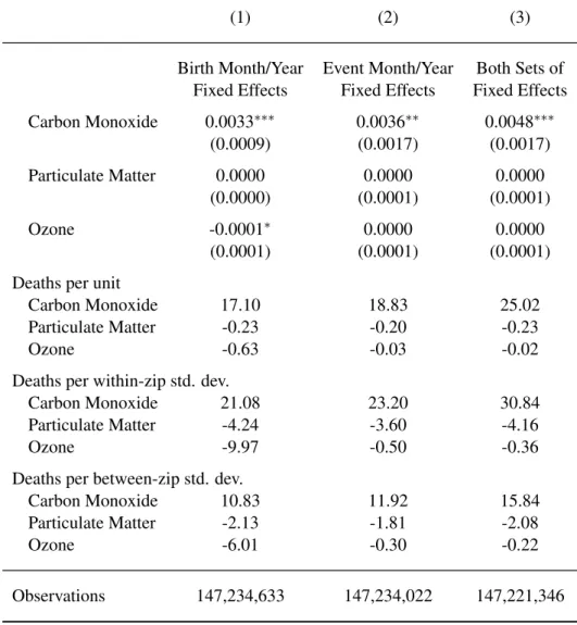
In column 2 we change the definition of the key time dimension for our fixed effects. In this panel define the fixed effects based on month-year of period alive and at risk to die, rather than of month-year of Birth. Note that the use of a different fixed effects specification results in a slightly different sample size, as singleton observations within fixed effects cells occur at different rates. An in column 1, our fixed effects are defined at the zip-by-month-year level. Results are largely similar to column 1, though slightly larger for CO and ozone is no longer marginally significant. Finally, in column 3 we use all sets of fixed effects, or
zip-by-month-of-birth-by-year-of-birth-by-month-of-life-by-year-of-life. Results are substantially larger for CO and unchanged for PM10 and ozone — a one-unit change in CO now causes an increase of 25 deaths per 100,000 live births. As a point of comparison, we also include the marginal impacts of an increase of a within-zip code standard deviation and a between-zip code standard deviation.
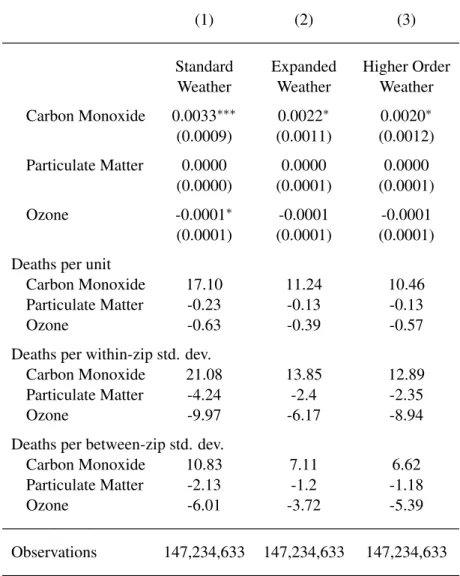
Next we examine the robustness of these results to adding more weather control variables. These variables may be correlated with infant health, and are conceptually important control vari-ables in our instrumental varivari-ables model. CN include maximum weekly temperature and weekly rain totals. Column 1 of Table 4 is again our replication of the CN results using our estimation method. In column 2, we add linear controls in the additional weather variables of specific hu-midity, windspeed, days with rain, and days with fog. While the coefficient has decreased by approximately 33%, it remains marginally significant. Addition of our higher order (up to cubic) terms in all weather variables (column 3) leaves findings largely unchanged.
Overall, we interpret the findings in Tables 3 and 4 as confirming that our methodological approach can replicate the initial findings in CN. Our findings also suggest that the timeframe choice of fixed effects is relatively inconsequential. However, the relationship between certain ambient weather variables and pollution may be a potential source of bias in estimating the effects of pollution on health factors.
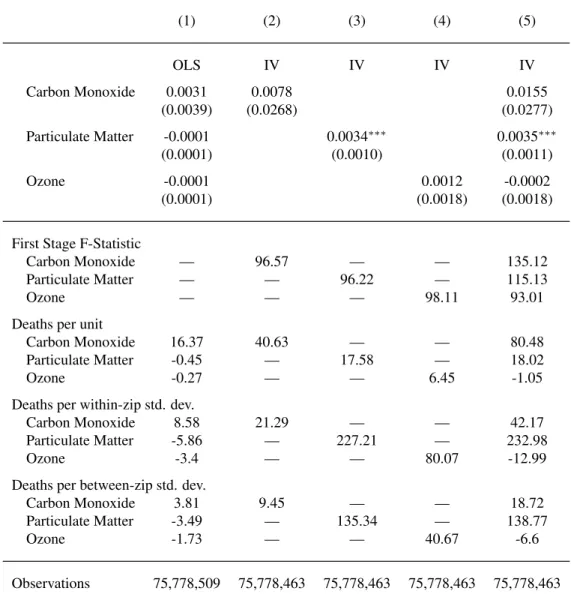
We next consider the time period from 2002 to 2007. In this period average CO levels are 40% below those from 1989 to 2000, average levels of PM10 are 5 percent lower, and O3 levels are 3 percent lower. Results are presented in column 1 of Table 5. This specification includes zip-by-event time fixed effects and cubics in all weather terms. Overall, our estimates are consistent with those from the earlier period, but are estimated with greater noise. As such we are unable to rule out zero effects. The point estimates, however, imply similar conclusions — CO is most correlated with infant mortality, and PM10 and O3 less so. A one unit decrease in CO saves 16.37 lives, an estimate surprisingly close to the CN result given the substantially lower CO levels in our time period. The comparison across the two time periods suggests a potentially concave damage function for CO’s impact on infants. However, our estimates have large standard errors and we cannot reject zero effect in the modern timeframe. Note the difference in standard deviation impact numbers, as a one-unit change in CO at today’s lower levels represents a substantially greater relative change.
5.2
First stage: Traffic and pollution
Our first stage model utilizes traffic and traffic interacted with linear and quadratic terms in weather variables as the main instruments. As such the estimated marginal effects are difficult to interpret. Instead, to give a sense of the first stage results and the intuition behind the interactions with weather, we present a graphical summary. The first stage model yields predictions of traffic’s impact on each pollutant, and this impact varies with weather conditions. This variation implies a distribution of the derivative of each pollutant with respect to our traffic measure, since the different observations in our data experience different weather.
To gain further insight into whether our measure of traffic correlates with pollution in ways that make sense, we stratify our “first stage” estimates based on weather. We choose example splits that we think (based on the atmospheric chemistry) should result in a clear distinction between con-ditions where traffic should have greater impact on pollution, and concon-ditions where traffic should have less of an impact on pollution.
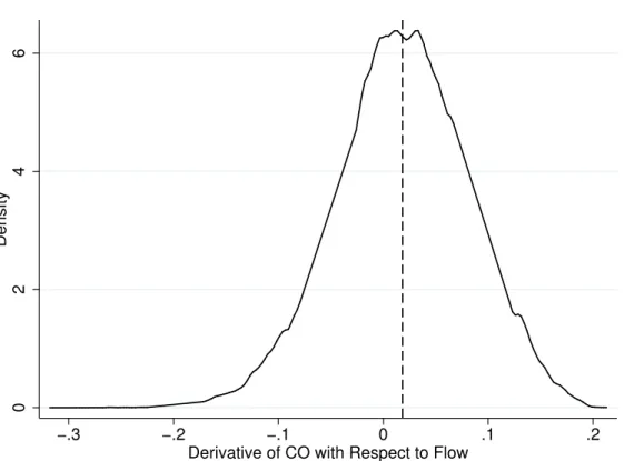
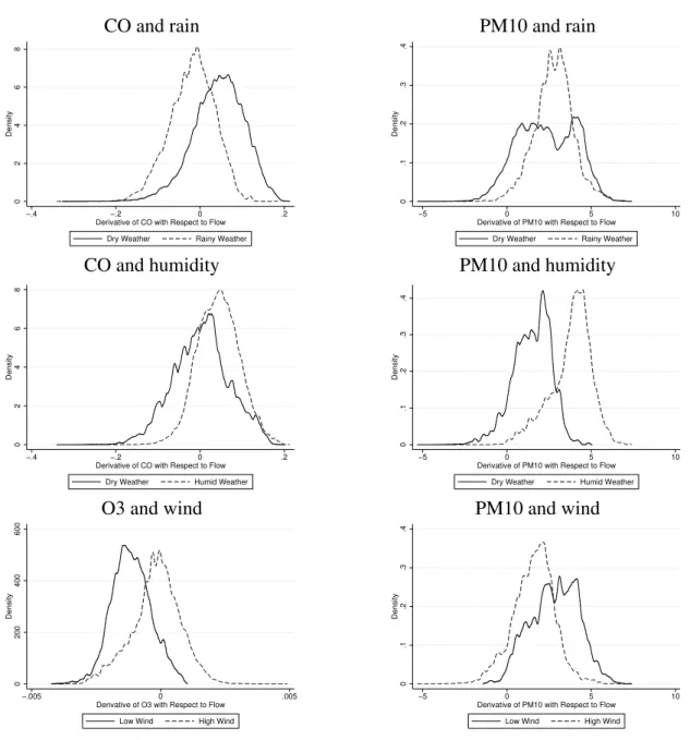
Figure 1 shows that traffic typically increases CO, and a majority of the distribution is positive. However, the magnitude of the average impact is low, and a large portion of the distribution is negative. We are hesitant to draw too much inference from the sign of these effects, however, due to the presence of our zip-by-month-by-year fixed effects, which make the marginal effects more difficult to interpret. More important to our identification strategy is the use of weather interactions and how changes in weather patterns shift the distributions in intuitive ways. We plot the marginal effect distribution across different weather conditions, splitting results by particularly “low” condi-tion days (below the 25th percentile for that particular weather variable) and “high” condicondi-tion days (above the 75th percentile). For example, graph (a) of Figure 4 suggests that increases in traffic have less of an impact on CO when the number of days with rain is above the 75th percentile, and graph (c) suggests slightly more of an effect when weekly humidity is above the 75th percentile.
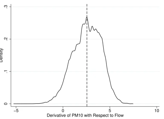
Figure 2 plots the distribution of the derivative of PM10 with respect to traffic. Nearly the entire distribution is positive. We also see intuitive shifts in the distribution with changes in weather conditions. The effect of rain and humidity on the relationship between PM10 and traffic contrasts to that of CO. Rainfall does not appear to influence the mean relationship between traffic and PM10 levels though it does impact the overall distribution shown in graph (b) of Figure 4, and humidity greatly increases this relationship for PM10.
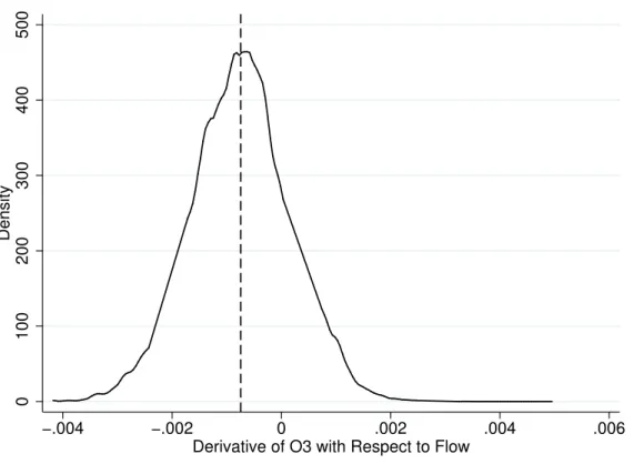
As with CO a large fraction of the derivatives are negative (58 percent). This is not surprising in the case of ozone, since traffic generated nitrogen oxides and VOCs are components in both the formation and titration of ground-level ozone (see Section 3). Graph (e) of Figure 4 shows that higher wind levels result in higher ozone levels, possibly due to greater circulation of chemicals in the air, providing more opportunities for chemical reactions, or because higher wind levels mean clouds move more quickly and sunlight is allowed in more frequently. Graph (f), however, shows that high winds result in lower PM10 values as the wind keeps air cycling and prevents the temperature inversion atmospheres that favor higher PM10 levels.
In summary, the marginal impact of additional traffic varies by ambient weather conditions, and varies differently by pollutant. This variation provides us with additional first stage power. Additionally, it offers a means by which to separately identify the effect of each pollutant on infant mortality in the second stage.
5.3
Instrumental variables estimation
Our main instrumental variables estimates are reported in Tables 5. For all IV regressions, first-stage F statistics are included below reported coefficients, as are marginal effects. As noted above, our instrumentation strategy uses interactions of traffic and ambient weather conditions, and use fixed effects for mother’s zip by month of event and year of event. While the year of birth is likely to affect mortality by capturing unobserved year-specific variables during pregnancy and the first portion of life, we believe that unobservable variables during the current month and year of life are also likely to be important. PM10 is the only pollutant that is statistically significant, and remains so when including all three pollutants simultaneously. The coefficients suggest that a one-unit decrease in PM10 is associated with approximately 18 fewer deaths per 100,000 live births, while a within-zip standard deviation in traffic is associated with 233 additional deaths.
In considering the magnitude of these effects, it is helpful to refer to prior findings on particulate matter and infant mortality rates. For example, Chay and Greenstone (2003b) find that a one unit drop in total suspended particulates (TSPs) resulted in a drop of 4-8 infant deaths per 100,000 live births, while Chay and Greenstone (2003a) found an effect of around 7-13 infant deaths per unit. Both analysis used TSPs, which contain both PM10 and larger particulates not included in the PM10 specification. While no direct conversion metric exists, the The World Bank Group note a commonly used conversion metric between the two measures is PM10 = 0.55 · T SP (The World
Bank Group (1999)). Using that conversion metric, the Chay and Greenstone (2003a) results suggests marginal impacts of 7-15 and 13-23 additional deaths per unit increase of PM10. Our results fall squarely within these estimates. However, we note those were based on yearly averages, which no doubt included both substantially higher and lower weekly values.
5.4
Robustness Checks and Extensions
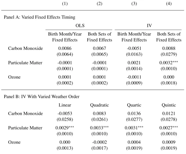
We first examine the robustness of our results to the time definitions of the fixed effects. In Table 6, we show that results are largely consistent across fixed effects specifications, though results are weaker when we do not include event month by event year effects. This suggests event time fixed effects are important in identifying the true effect of traffic on pollution.
We also examine the sensitivity of our results to the specification of the weather control vari-ables. In panel B of Table 6, we show that our results are robust to all polynomial orders from linear to through quintic.
One of the benefits of using interactions between weather and traffic as instrumental variables is the ability to jointly identify the impacts of three separate pollutants despite only having one measure of traffic. However, the use of multiple instruments raises the concern of the true source of identification. Are our results a product of simply using enough instruments to get a statistically significant result? Or are results being driven by the inclusion of a particular weather effect alone? Both of these issues are of concern. To address this, we repeat our main IV analysis but vary the weather interactions included in the first stage. Results are shown in Table 7. As we begin with fewer than three instruments, we cannot estimate the simultaneous pollutant model, so we instead conduct all analysis in a single-pollutant framework.
Column 1 shows results from using only traffic as an instrument with no additional weather interactions. Column 2 adds an interaction with temperature, column three adds an additional interaction with humidity, and so on. The lower panel indicates which weather interactions are included for each column. By column 7, the regressions are equivalent to columns 2, 3, and 4 in Table 5. Results for both carbon monoxide and ozone are never statistically significant at conven-tional levels and shift between being positive and negative. The effects for PM10, however, are always positive. And while the estimates using only traffic as an instrument are not statistically significant, they are within a single standard error of the results in the most saturated model. Look-ing across all specifications, it does not appear that the addition of any sLook-ingle pollutant explains the
size or magnitude of our results. Results become much more precisely estimated with the addition of humidity to the interaction set, suggesting there may be a strong link between ambient humidity, traffic, and pollution.
To summarize, our modern OLS results are similar in magnitude to those found during the 1989-2000 period, though the standard errors are too large to reject zero effects for any pollutants. Within the IV models we find a robust relationship between infant health and particulate matter levels, but do not find evidence that carbon monoxide and ground-level ozone adversely impacts infant mortality. The findings with PM10 do not appear to be driven by the use of a large number of instruments.
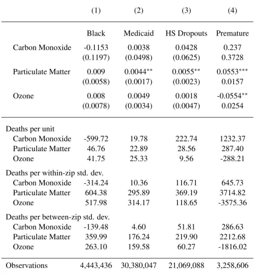
We next consider how the impacts of pollution might vary across different subgroups. We consider effects separately for blacks, births covered by Medicaid, births to high school dropouts, and premature infants. Results are shown in Table 8. For all subgroups, effects are larger than the average effect in Table 5. The effect for blacks (column 1), while almost three times the mean impact, is not statistically significant, possibly due to the much smaller sample; only around 6% of observed births during the 2002-2007 period are to black mothers. Effects for births funded by Medicaid and births to high school dropouts are approximately 25% and 60% larger than mean effects, respectively. Most puzzling, however, is the result for premature infants. Estimated effects of PM10 are over 10 times that for the average population. However, effects for ozone are similarly large and have a counterintuitive negative sign. This could be a product of toxicity of ozone component pollutants. For example, higher ozone levels are likely correlated with lower nitrogen oxide levels. This could also be a byproduct of the small sample chosen, where fewer than 5% of births are premature. Another possibility is the impact of prenatal pollution exposure. Premature infants may be premature due to higher pollution levels during gestation, and if pollution is strongly correlated over short periods of time that could complicate our estimation. This is particularly important as premature infants that die within a year do so quickly, with approximately 45% dying in the first week of life and 60% of deaths occurring in the first two weeks of life (versus 30% and 43%, respectively, for the full sample). Regardless of the reasoning, the exceptionally large coefficient on PM10 and the negative, statistically significant sign on ozone make us wary of attempting to interpret the findings for prematurely born infants.
5.5
Reduced form results
As with the first stage, the interaction of traffic with weather conditions implies a distribution of reduced form effects of traffic on infant mortality. An F-test of the joint statistical significance suggests fairly precisely estimated effects (p-value of 0.008), but the interpretation of individual coefficients, as in the case of the first stage estimates, is complex. However, the distribution of impacts is intuitive. Figure 5 is a kernel density estimate of the joint effect of a marginal change in traffic on infant mortality. We calculate this by regressing the weekly mortality rate on all co-variates in our main specification as well as traffic and our interactions. For each observation, we then generate an estimated marginal impact of traffic and mortality for that observation’s given weather conditions, and then plot the density of those effects. To aid in interpretation, we plot the percentage change in the infant mortality rate for a change in traffic equal to a within-zip code stan-dard deviation. While the density shows some negative values, the majority of observations find positive values with a mean of approximately 0.006. This suggests a standard deviation increase in our weekly traffic measure raises the probability of an infant death in that week by approxi-mately 0.0007 percentage points. Over a 52-week period, this translates to a 0.04 percentage point increase, or a change of approximately 14% of the baseline.
We next investigate how the reduced form is affected by changes in weather conditions. This is driven by two primary thought experiments. First, just as we expect the impact of traffic on pollution to vary with ambient weather, we would also expect the reduced form impact of traffic on mortality to vary with weather conditions. Second, as noted above weather itself has been shown to have a substantial impact on mortality independent of traffic. Figure 6 plots the kernel density estimates of the impact of traffic on mortality in various weather conditions (note again we have dropped all deaths associated with auto trauma to insure that our results are not driven by mortality in auto accidents caused by weather conditions). Panel A of Figure 6 shows the density for all expanded births, and then separately for weeks with high rain and weeks with high fog (where high is again defined as greater than the 75th percentile). Panel B again shows all expanded births, along with weeks with high humidity, high temperature, and high wind.
Taken cumulatively, the graphs suggest that the reduced form is largest during humid weeks and weeks with high fog. This is consistent with our results that traffic has a stronger effect on PM10 during such conditions, and PM10 has a stronger influence on infant mortality in our period of analysis. When we compare the weeks with rain versus those without, we see only slightly higher effects during rainy conditions. The effect of traffic on infant mortality subsides considerably
during windy periods, possibly because high winds clear the air and prevent temperature inversion. Finally, we find little variation by temperature.
We next analyze whether the reduced form relationship changes with demographics. We con-tinue to use the average of one standard deviation in traffic within zip codes. Panel A of Figure 7 plots kernel density estimates of the reduced form across all observations, black mothers and His-panic mothers. Panel B repeats all observations, and includes high school dropout mothers, births covered by Medicaid, and premature births. The estimate is slightly larger for Hispanic mothers, and effects for blacks are noisy and the mass is negative. As noted in Table 8, blacks make up a small portion of the birth population and have a statistically insignificant second stage estimate as well. Results appears slightly smaller for Medicaid patients, which is surprising given the larger second stage effects found in Table 8. Effects for high school dropout mothers are much larger, and largest is the effect for premature infants. The particularly wide distribution for premature infants is interesting this may be a factor of very early births being treated in the hospital early on in life, preventing the most extreme cases from being exposed to outdoor pollution levels.
In summary, the reduced form estimates suggest that shocks to traffic congestion result in in-creases in weekly infant mortality rates. These effects are strongest during periods of high humidity and high fog, and lowest during periods of high wind, suggesting conditions that favor high partic-ulate matter levels are more likely to increase mortality rates. Effects are also largest for Hispanics, premature infants, and infants born to mothers that did not finish high school. Effects for blacks are particularly noisy, perhaps due to the small number of births.
6
Conclusions
We contribute to the existing literature on pollution and health by analyzing the impact of car-bon monoxide, particulate matter, and ozone on infant health, as was done by Currie and Neidell (2005). We first consider how their results vary with econometric specifications, and then illustrate the importance of weather in the estimates of pollution’s impacts on health. This suggests that weather may be of substantial importance in the estimation of pollution and health effects.
We next consider the impacts of the lower pollution levels seen in California today. We find effects are similar in magnitude to those in the 1989-2000 period, though are no longer statistically significant. There are a number of reasons to be concerned that OLS would yield inconsistent
estimates of the impact of pollution on infant health. First, mothers may self-select into geographic regions. Second, changes in local economic activity may also bias OLS estimates. Third, pollution is likely measured with error. The majority of papers in this literature assign pollution levels to a particular person, living in a particular geographic area (e.g., zip code or county), based on pollution readings from pollution sensors in or near this geographic area. This introduces three sources of measurement error. We instrument for pollution using weekly shocks to traffic and its interactions with ambient weather conditions as a potential correction to these problems, and in doing so consider a relationship between traffic congestion and infant mortality.
We find PM10 has a large and statistically significant effect on infant mortality, while there is little stable evidence on the relationship of carbon monoxide or ozone infant health. Considering the substantial decrease in ambient carbon monoxide levels in the past 15 years, this is not entirely surprising. In our preferred specification, a one-unit decrease in PM10 (around 13% of a standard deviation) saves roughly 18 lives per 100,000 births. This represents a decrease in the mortality rate of around 6%. This is consistent with the findings of prior research on ambient particulate matter, and suggests that even at today’s lower levels are substantial health gains to be made by reducing both ambient pollution and traffic congestion.
References
ALMOND, D., L. EDLUND, AND M. PALME (2009): “Chernobyl’s Subclinical Legacy:
Prena-tal Exposure to Radioactive Fallout and School Outcomes in Sweden,” Quarterly Journal of Economics, 124, 1729–1772.
BARRECA, A. (2008): “Climate Change, Humidity, and Mortality in the United States,” Mimeo.
BISHOP, G. AND D. STEDMAN(1996): “Measuring the Emissions of Passing Cars,” Acc. Chem.
Res, 29, 489–495.
BRAUER, M., G. HOEK, H. SMIT, J. DEJONGSTE, J. GERRITSEN, D. POSTMA, M. KERKHOF,
ANDB. BRUNEKREEF(2007): “Air pollution and development of asthma, allergy and infections
in a birth cohort,” European Respiratory Journal, 29, 879.
BRUNEKREEF, B., N. JANSSEN, J. DE HARTOG, H. HARSSEMA, M. KNAPE, AND P. VAN
VLIET(1997): “Air pollution from truck traffic and lung function in children living near
motor-ways.” Epidemiology, 8, 298.
CHAY, K. Y., C. DOBKIN,AND M. GREENSTONE(2003): “The Clean Air Act of 1970 and adult mortality,” Journal of Risk and Uncertainty, 27, 279–300.
CHAY, K. Y.ANDM. GREENSTONE(2003a): “Air quality, infant mortality, and the Clean Air Act of 1970,” NBER Working Paper No. 10053.
——— (2003b): “The Impact of Air Pollution on Infant Mortality: Evidence from Geographic Variation in Pollution Shocks Induced by a Recession,” Quarterly Journal of Economics, 118, 1121–1167.
CURRIE, J. (2011): “Inequality at Birth: Some Causes and Consequences,” Tech. rep., NBER
Working Paper 16798.
CURRIE, J., E. A. HANUSHEK, E. M. KAHN, M. NEIDELL,ANDS. G. RIVKIN(2009a): “Does
Pollution Increase School Absences?” The Review of Economics and Statistics, 91, 682–694.
CURRIE, J. AND M. NEIDELL (2005): “Air Pollution and Infant Health: What Can We Learn
From California’s Recent Experience?” Quarterly Journal of Economics, 120, 1003–1030.
CURRIE, J., M. NEIDELL, AND J. F. SCHMIEDER (2009b): “Air pollution and infant health:
CURRIE, J.ANDJ. F. SCHMIEDER(2009): “Fetal Exposures to Toxic Releases and Infant Health,” The American Economic Review, 99, 177–183.
CURRIE, J. AND R. WALKER (2011): “Traffic Congestion and Infant Health: Evidence from
E-ZPass,” American Economic Journal: Applied Economics, 3, 65–90.
DAVIS, S.ANDS. DIEGEL(2007): “Transportation Energy Data Book: Edition 26-2007,”
ORNL-6978. Prepared for the US Department of Energy. Oak Ridge, TN: DOE.
DESCHENESˆ , O. ANDM. GREENSTONE (2007): “The economic impacts of climate change:
ev-idence from agricultural output and random fluctuations in weather,” The American Economic Review, 97, 354–385.
——— (2011): “Climate change, mortality, and adaptation: Evidence from annual fluctuations in weather in the US,” Forthcoming in the American Economic Journal: Applied Economics. DESCHENESˆ , O., M. GREENSTONE, AND J. GURYAN (2009): “Climate Change and Birth
Weight,” The American Economic Review, 99, 211–217.
FRIEDMAN, M. S., K. E. POWELL, L. HUTWAGNER, L. M. GRAHAM, AND W. G. TEAGUE
(2001): “Impact of changes in transportation and commuting behaviors during the 1996 Summer Olympic Games in Atlanta on air quality and childhood asthma,” The Journal of the American Medical Association, 285, 897.
GAUDERMAN, W., H. VORA, R. MCCONNELL, K. BERHANE, F. GILLILAND, D. THOMAS,
F. LURMANN, E. AVOL, N. KUNZLI, M. JERRETT, ET AL. (2007): “Effect of exposure to
traffic on lung development from 10 to 18 years of age: a cohort study,” The Lancet, 369, 571– 577.
GRAFFZIVIN, J.ANDM. NEIDELL(2009): “Days of haze: Environmental information disclosure
and intertemporal avoidance behavior,” Journal of Environmental Economics and Management, 58, 119–128.
GRAFF ZIVIN, J., M. NEIDELL, AND W. SCHLENKER (2011): “Water quality violations and
avoidance behavior: Evidence from bottled water consumption,” Tech. rep., NBER Working Paper 16695.
LEE, S., A. COCCO, D. KEYVANI, ANDG. MACLAY(1995): “Humidity Dependence of Carbon Monoxide Oxidation Rate in a Nafion-Based Electrochemical Cell,” Journal of the Electrochem-ical Society, 142, 157.
LLERAS-MUNEY, A. (2010): “The needs of the Army: using compulsory relocation in the military
to estimate the effect of air pollutants on children’s health,” Journal of Human Resources, 45, 549.
MORETTI, E.AND M. NEIDELL(2011): “Pollution, Health, and Avoidance Behavior: Evidence
from the Ports of Los Angeles,” Journal of Human Resources, 46, 154–175.
NEIDELL, M. (2009): “Information, Avoidance Behavior, and Health: The Effect of Ozone on
Asthma Hospitalizations,” Journal of Human Resources, 44, 450.
NEIDELL, M. J. (2004): “Air pollution, health, and socio-economic status: the effect of outdoor
air quality on childhood asthma,” Journal of Health Economics, 23, 1209–1236.
PONCE, N. A., K. J. HOGGATT, M. WILHELM, ANDB. RITZ(2005): “Preterm birth: the inter-action of traffic-related air pollution with economic hardship in Los Angeles neighborhoods,” American Journal of Epidemiology, 162, 140.
REYES, J. W. (2007): “Environmental Policy as Social Policy? The Impact of Childhood Lead
Exposure on Crime,” The BE Journal of Economic Analysis & Policy, 7, 51.
SAMET, J., S. ZEGER, J. KELSALL, J. XU, AND L. KALKSTEIN (1998): “Does weather con-found or modify the association of particulate air pollution with mortality? An analysis of the Philadelphia data, 1973–1980,” Environmental Research, 77, 9–19.
SANDERS, N. J. (2011): “What Doesn’t Kill you Makes you Weaker: Prenatal Pollution Exposure
and Educational Outcomes,” SIEPR Discussion Paper 10-019.
SANDERS, N. J. AND C. STOECKER (2011): “Where Have all the Young Men Gone? Using
Gender Ratios to Measure the Effect of Pollution on Fetal Death Rates,” Mimeo.
SHUKLA, J., A. MISRA, S. SUNDAR, ANDR. NARESH(2008): “Effect of rain on removal of a
gaseous pollutant and two different particulate matters from the atmosphere of a city,” Mathe-matical and Computer Modelling, 48, 832–844.
STOECKER, C. (2010): “Chill Out, Mom: The Long Run Impact of Cold Induced Maternal Stress In Utero,” Mimeo.
THE WORLD BANK GROUP (1999): Pollution Prevention and Abatement Handbook, The
Inter-national Bank for Reconstruction and Development.
TIAO, G. AND S. HILLMER (1978): “Statistical models for ambient concentrations of carbon
monoxide, lead, and sulfate based on the LACS data,” Environmental Science & Technology, 12, 820–828.