Periodic solutions for soil carbon dynamics equilibriums with time-varying forcing variables

HAL Id: hal-00124048

https://hal.archives-ouvertes.fr/hal-00124048v2

HAL is a multi-disciplinary open access

archive for the deposit and dissemination of sci-entific research documents, whether they are pub-lished or not. The documents may come from teaching and research institutions in France or abroad, or from public or private research centers.

L’archive ouverte pluridisciplinaire HAL, est destinée au dépôt et à la diffusion de documents scientifiques de niveau recherche, publiés ou non, émanant des établissements d’enseignement et de recherche français ou étrangers, des laboratoires publics ou privés.

Periodic solutions for soil carbon dynamics equilibriums

with time-varying forcing variables

Manuel Martin, Stéphane Cordier, Jérôme Balesdent, Dominique Arrouays

To cite this version:

Manuel Martin, Stéphane Cordier, Jérôme Balesdent, Dominique Arrouays. Periodic solutions for soil carbon dynamics equilibriums with time-varying forcing variables. Ecological Modelling, Elsevier, 2007, XXX (XXX), pp.XXX. �10.1016/j.ecolmodel.2006.12.030�. �hal-00124048v2�

Periodic solutions for soil carbon dynamics equilibriums

1

with time-varying forcing variables

2 3

Manuel Pascal Martin1, Stéphane Cordier2, Jérôme Balesdent3and Dominique Arrouays1. 4

1_{INRA, Unité Infosol, 2163 Ave Pomme de Pin, BP 20619, F-45166 Olivet, France}

5

2_{MAPMO UMR CNRS 6628 Université d’Orléans 45067 Orléans France.}

6

3_{LEMIR, UMR 6191 CEA Cadarache 13108 St Paul lez Durance France.}

7

Abstract

8

Numerical models that simulate the dynamics of carbon in soil are increasingly used to 9

improve our knowledge and help our management of the carbon cycle. Calculation of the long 10

term behavior of these models is necessary in many applications but encounters the difficulty 11

of managing the periodic forcing variables, e.g., seasonal variations, such as carbon inputs 12

and decomposition rates. This calculation is conventionally done by running the model over 13

large time durations or by assuming constant forcing variables. Two methods, which make it 14

possible to rapidly compute periodic solutions taking into account the time variations of these 15

variables, are proposed. The first one works on discrete-time models and the second one on 16

continuous-time models involving Fourier transforms. Both methods were tested on the 17

Rothamsted carbon model (RothC), a discrete-time model which has also been given a 18

continuous approximation, using realistic an unrealistic sets of time-varying forcing functions. 19

Both methods provided an efficient way to compute the periodic solutions of the RothC 20

model within the application domain of the model. Compared to running the discrete model to 21

the equilibrium, reduction in the computational cost was of up to 95% at the expense of a 22

maximum absolute error of 1% for the estimation of carbon stocks. For specific distributions 23

of the forcing variables the use of Fourier transform of zero order, which was equivalent to 24

assume constant forcing variables, led to a maximum absolute error of 55% in the estimation 25

of the long term behavior of the model. There, a Fourier transform of order higher than zero is 26

required. 27

Keywords: soil organic carbon dynamics, discrete formulation, continuous formulation, 28

steady state, periodic solutions, linear model, Fourier series. 29

Introduction

30

1.1. carbon dynamics

31

The soil organic carbon (SOC) plays an important role in several environmental and land 32

management issues. One of the most important issues is the role that SOC plays as part of the 33

terrestrial carbon and might play as a regulator of the atmospheric CO2. Many factors are 34

likely, in a near future, to modify the SOC content, including changes in agricultural practices 35

(Betts, 2000; Vleeshouwers and Verhagen, 2002; Bellamy et al., 2005) and global climate 36

changes (Jenkinson et al., 1991; Cao and Woodward, 1998; Cox et al., 2000; Jones et al., 37

2005; Knorr et al., 2005). Understanding SOC and soil organic matter (SOM) dynamics as a 38

function of soil characteristics, agricultural management and climatic conditions is therefore 39

crucial, and many models have been developed in this perspective. Most models of SOM 40

turnover, excepting a few (Bosatta and Agren, 2003), are compartmental models, exhibiting 41

various degree of complexity. The compartments represent carbon originating from plants or 42

contained in soil and transformed by microorganisms and each one is characterized by a 43

particular decomposition rate representing more labile or more stable forms of soil organic 44

matter. Some models include N turnover and/or plant growth modules (CENTURY) when 45

others only focus on SOC (RothC). Also, most use a linear method of transferring quantities 46

between the different compartments (Baisden and Amundson, 2003) but some models 47

including non-linear dynamics have also been developed more recently (Manzoni et al., 48

2004). 49

These models are used in a variety of ways and often for long term studies (Coleman et al., 50

1997; Falloon and Smith, 2002; Franko et al., 2002; Shevtsova et al., 2003; Shirato, 2005; 51

Shirato et al., 2005b; Shirato and Yokozawa, 2005a). The behavior of the SOC system, over a 52

long term and assuming that the environment of the system (inputs of organic carbon, climatic 53

conditions) is stable, is reported to tend toward a steady state. Although many soils under 54

study might not have reached equilibrium, being able to compute and predict the long-term 55

solution is extremely valuable. It gives a synthetic view of the system in given agro-climatic 56

conditions, makes it possible to test if a studied soil has reached an equilibrium or not, to 57

envision what would be the consequences of specific events onto a given soil assuming that a 58

new stable state is reached and to serve as a control case or initial conditions (Thornton and 59

Rosenbloom, 2005). Technically, the equilibrium assumption is also commonly used to solve 60

analytically mathematical systems. Such an analytical solution gives an explicit relationship 61

between model inputs and outputs and may, in turn, be computed without simulating or 62

integrating numerically the system until it reaches a stable state, thus saving computation 63

time. When models cannot be formulated analytically, estimating the steady state solutions 64

still can be useful and generic or model specific efficient numerical methods are available 65

(Thornton et al., 2005). More generally, being able to use analytical forms of the long-term 66

solutions is particularly useful in understanding models behavior and relationships between 67

input and output variables of the model. 68

Some of the SOC models have been formulated mathematically (Parshotam, 1996; Bolker et 69

al., 1998; Yang et al., 2002; Baisden et al., 2003; Manzoni et al., 2004) and approaches, as the 70

development of the ICBM family models (Katterer and Andren, 2001), specifically aim at 71

proposing analytically solved models representing the conventional wisdom of soil C and N 72

modelling. For these models, when studying N and C soil content at steady state, it is usually 73

assumed that forcing variables (typically climatic variables and variables representing inputs) 74

can be set to their average value, calculated over a representative year for instance, which 75

considerably eases the mathematical treatment. There, the long-term behavior of the model 76

truly is a steady state. Consequences of such an assumption have for now been tested only 77

empirically for some models and specific conditions. In some cases, environmental shifts 78

from one stable state to another or brief events are considered and mathematical treatment 79

used to estimate the new stable state after perturbation or the system resilience. We propose 80

here two methods which make it possible to deal with continuously time varying agro-81

climatic conditions (e.g. forcing variables), when they can be specified as periodic functions. 82

The first one works on discrete-time models and the second one on continuous-time models 83

involving Fourier transforms. We considered the Rothamsted model with crop cultivations, as 84

representative of many models of soil organic matter dynamics, anticipating that the second 85

method could also be applied to models involving non-linear dynamics. We used these 86

methods to test the consequences of assuming yearly constant agro climatic condition instead 87

of considering their intra-annual variability. 88

Methods

89

1.2. Discrete formulation

90

The RothC model (Coleman et al., 1997) splits the soil carbon into four active compartments 91

and one inactive. At each time step, the four active compartments, decomposable plant 92

material, DPM, resistant plant material, RPM, the microbial community BIO and the humus, 93

HUM, undergo decomposition as a function of a rate constant, depending on the compartment 94

and on a rate modifier. The rate modifier depends on the clay content of the soil, climatic 95

variables and land cover. Products of the decomposition are CO2 and carbon feeding the BIO

96

and HUM compartments. The fraction of the decomposed carbon incorporated into BIO and 97

HUM increases as a function of the clay content of the soil. Carbon enters the soil through the 98

DPM and RPM compartments. The fraction input in DPM and RPM respectively is chosen as 99

a constant which is an estimate of the decomposability of the plant material. It depends on the 100

cultivation being considered. The model can be formulated as 101 t t t t FC B C_1   Where 102 t t hum bio rpm dpm C                                                   hum t hum t bio t rpm t dpm t hum t bio t bio t rpm t dpm t rpm t dpm t k ρ k ρ k ρ k ρ k ρ k ρ k ρ k ρ k ρ k ρ k ρ k ρ t e e e e e e e e e e e e F ) 1 ( ) 1 ( ) 1 ( ) 1 ( ) 1 ( ) 1 ( ) 1 ( ) 1 ( 0 0 0 0 0 0         and 103 dpm rpm t t bio hum a a B b a a             

The four input coefficients (adpm, arpm, abio and ahum) sum up to 1 and in the most common case

104

one uses adpm=γ , arpm=1-γ, abio=0 and ahum=0, γ depending on the quality of the plant

105

material. 106

Here, α and β are fractions of metabolized C incorporated respectively into BIO and HUM. bt

107

is the carbon amount (t.ha-1) entering the system at month t, ki the decomposition rate for

108

compartment i and ρt the rate modifier.

Characterization of the long-term behavior

110

In case where bt and ρt are constant, one can demonstrate that the (I4-F) matrix, where the

111

matrix I4 is the 4-by-4 identity matrix, has an inverse (see below) and that the system yields a

112

steady state solution. Assuming that F and B are respectively the time constant carbon flows 113

and carbon inputs, one can write 114

4

* _{( )} 1

C  I F  B

However, usually Ft and Bt vary through time but it can be assumed that they have a periodic

115

behavior. Typically, if the agronomical practices are cyclic and if the weather conditions can 116

be considered as periodic, ρt, bt, and consequently Ft, Bt will also behave periodically.

117

Assuming that the periodicity of these variables is P, one looks for a solution of C such that 118

t P t

C_ C (1)

For example, considering the common case the case where P is 12 months, we can write 119 down 120 12 11 12 11 10 11 11 1 1 1 .. B C F C B C F C B C F C t t t t t t          

which can be reformulated as: 121 4 1 1 2 10 10 4 11 11 11 4 12 12 0 0 0 0 0 0 0 0 0 0 0 0 0 0 0 t t t t t t C C I F B F C C I B C C I F B                                                                                                                 (2)

and finally yields: 122 1 1 4 1 2 4 4 11 4 12 12 0 0 0 0 0 0 0 t t C F I B F I I C I F B             _                   _                _                      (3)

Solving this system (which can be performed via matrix inversion by common statistical 123

packages or spreadsheet programs) yields a vector of dimension 4*12, which is the sequence 124

of states Ci=(dpmi, rpmi, bioi, humi)T, i in |[1,12]| and which characterizes the oscillatory state

125

of carbon stock in each compartment, keeping track of the temporal variability of the forcing 126

variables over the period. 127

1.3. Continuous formulation

128

In real soil systems, processes involved in the RothC model are continuous in time and thus 129

one can propose the following continuous formulation, where C’ denotes the derivative of C 130

with respect of time: 131 ) ( ) ( ) ( ) ( ' t t AC t B t C    (4) with 132                    hum bio rpm dpm hum bio rpm dpm rpm dpm k k k k k k k k k k A ) 1 ( ) 1 ( 0 0 0 0 0 0         (5)





ρ(t) is the decomposition rate modifier. In the current RothC formulation, ρ(t) is a function of

133

monthly rainfall, temperature, pan open evaporation and land cover, as well as percentage of 134

clay in the considered soil. When the time varying input variables (climatic and agricultural 135

variables) are considered as periodic functions of period P, ρ(t) itself is a periodic function 136

with the same period. b(t) is considered on a periodical basis too, as for the discrete 137

formulation of the model. Again, the system defined by C(t) is expected to tend toward a 138

oscillatory state as t→+∞. Study of the eigenvalues of ρ(t)A enables to characterize such a 139

behavior. Let us define y(t) and A(t).

140

( )

( ) t ( )

y t _eA C t ₍₆₎

where A(t) is the primitive of ρ(t)A .

141

From Eq.(4) and (6) we obtain 142 ( ) '( ) t ( ) y t _eA B t and 143 ( ) 0 ₀ ( ) t s ( ) y t y 



Setting _{A(0) to the four by four zero matrix, from Eq.(6) and (7) it can be written} 144

( ) ( ) ( )

0 ₀

( ) t t t s ( )

C t eA C eA



We can first observe that if _{A(t) eigenvalues are negative, C(t) as t→+∞ do not depend on} 145

initial conditions C0. Secondly, if C(t) has a periodic solution, say C0, with period P, it can be

146

shown using semigroup representations that it satisfies the following Equation, 147 ( ) ( ) ( ) 0 0 ₀ ( ) T T T s C _eA C _eA



A solution to this equation exists and is unique if (Id-e -A(t)_{) has an inverse, which can be}

148

demonstrated to be true if A is invertible. A sufficient condition for A to be invertible is that 149

all its eigenvalues are nonpositive, i.e. using the definition of A (Eq.(5)) when α+β<1. This 150

condition is always true for the RothC model due to the definition of α and β (Coleman and 151

Jenkinson, 1995) and thus the stock of carbon in each compartment tends towards a periodic 152

solution in large times whatever the input values are. 153

Characterization of the long-term behavior

154

Approximations of this behavior can be made using Fourier series. Setting 155 ( ) N ikt N k k N C t C e  











ρk and bkcoefficients can be obtained from the monthly input values used in the RothC model.

157

C(t), A(t) and B(t) can be replaced by their respective Fourier transform in Eq.(4) giving the

158 following approximation. 159 ( ) , / N N N ikt i j k t ikt k j k k k N j k j k N k N ikC e A C  e  b e      







Setting N, the order of the Fourier series, to zero, we calculate the C0 term.

160 0 0 1 0 A B / C    (9)

Assuming that B0 = (γ, 1- γ, 0, 0)T.b0, which means that carbon inputs only to the DPM and

161

RPM compartments, leads to the following solution: 162

                  ] ) 1 /[( ] ) 1 /[( / ) 1 ( / 0 0 0 0 0 0 0 0 0 hum bio rpm dpm k b k b k b k b C             (10)

b0 and ρ0 terms represent averages of b(t) and ρ(t) over the considered period, which is one

163

year. This solution gives an explicit formulation of the long-term behavior of the system, 164

which obviously equals what would have been found using the assumption of constant forcing 165

variables set to the average values. This solution does not enable to takes into account the 166

temporal variability of the carbon stocks throughout the year. This could have been achieved 167

by computing the C1 term which itself is an approximation of the primary oscillations of the

168

system’s long-term behavior. Such a calculation lies beyond the scope of this paper. These 169

oscillations directly depend on the temporal variability of the forcing variables but their size is 170

usually small compared to the total SOC. In the following, they will be handled only with the 171

discrete formulation of the RothC model (Eq.(3)). 172

1.4. Comparison of the approaches

173

Parshotam (1996) showed that given some restrictions the continuous formulation (Eq.(4)) is 174

a good approximation of what would be the continuous formulation of the original discrete 175

time RothC model. It is possible to turn this the other way round and say that the RothC 176

model is an approximation of the discretization of the continuous model given in Eq.(4). 177

Discretization of Eq.(4) leads to, in case of constant inputs during the sampling intervals 178 (Parshotam, 1996): 179 ( ) 1 ( ) ( 1) ( ( ) ) ( 4) ( ) k t A t k t A t k t k t C _{ } e  C _   k t A  e   I B k t

RothC is an approximation of the above equation because 180 (k t A t) t F _e   _and 1 ( ) 4 ( ( ) ) ( k t A t ) ( ) t B _  k t A_  e   _I B k t_

Thus, the parameters used in the continuous model (e.g. α, β, kdpm, krpm, kbio and khum) should

181

not be equated with those of the RothC model. However, numerically it makes little 182

difference, and in the following developments, we shall do it. 183

Both approaches (using the discrete or the continuous formulation) can be used to 184

characterize the periodic long-term behavior of the system. The first approach (Eq.(3)) uses 185

the discrete formulation of the model which formally reproduces the specification of the 186

RothC model contrary to the second one (Eq.(9)) which uses a continuous formulation and a 187

zero order Fourier transform. This latest approach gives a simpler explicit solution, function 188

of the input variables and parameters of the model (α, β, kdpm, krpm, kbio and khum). It might also

189

be more interesting to work with the continuous form of the model because of its greater 190

generality and since it is usually easier to discretize a continuous model rather than doing the 191

opposite. 192

To assess the validity of both approaches in characterizing the long-term behavior with time-193

varying forcing variables, we first compared both approaches between themselves and with 194

the discrete model where variability of forcing is leveraged over the year. This was performed 195

using a weather dataset composed by monthly averages calculated over 12 years (1992-2004) 196

on a 0.125° grid (4144 cells) covering the French country. For each point of the grid, we 197

considered a unique crop system, with inputs being 0.50, 0.20, 0.10, 0.10, 0.10, 1.44 tC.ha-1 198

respectively for each month from March to August, otherwise null with a bare soil (adapted 199

from Swinnen et al., 1995 and Bolinder et al., 1997 for winter wheat). %Clay was set to 10%. 200

The computation of the long-term behavior using the discrete formulation resulted in a 201

periodic solution, i.e. a sequence of twelve Ci states, i in [1..12] (Eq.(3)). The solution given

202

by a discrete formulation with averaged forcing variables was a single state noted Cavg , the

203

calculation obtained using the continuous formulation was also a single state, noted C0

204

(Eq.(9)). We compared Cavg, with C0and with the average state of the Ci states, noted <Ci>.

205

To test more systematically the validity of the estimator based on Fourier series introduced in 206

(Eq.(8)), e.g. C0, the periodic solutions were also computed when varying the forcing

207

variables independently, using in some case extreme and unrealistic values. The precision of 208

C0 was assessed using the σ/C0 ratio, where σ is the standard deviation of the Ci states and

209

represents the size of the oscillations characterizing the periodic solution. The bias of C0 was

210

assessed using the abs(<Ci>-C0)/C0 ratio. We modeled the distributions of the forcing

211

variables using Gaussian functions as 212 a d N d N y y i i i i  



Where yi, i in [1..12] is the value of the forcing variable (either b(t) or ρ(t)) at month i, a and d

213

respectively the amplitude and dispersion characterizing the distributions, and ymin a minimum

214

value for the considered variable. Low values of the d parameter yielded distributions having 215

a spike around the sixth month, high values uniform distributions. The a parameter 216

represented a scaling parameter. a and d were varied at once and sampled linearly within their 217

range of variation. ymin and the range of variation of d and a were, respectively for b(t) and

ρ(t), (0.1, [0.1,5] and [0.1,10]) and (0.83, [0.1,5] and [0.1,100]). One forcing variable

219

remained constant whilst the amplitude and dispersion of the other was varied and set to 0.2 220

for bi, i in [1..12] and set to 0.8, 0.8, 0.8, 0.82, 1.06, 1.10, 1.06, 0.82, 0.8, 0.8, 0.8, 0.8 for ρi, i

221

in [1..12]. 222

To compute the solutions with both approaches, the calculation of modifiers of the 223

decomposition rates was done using SQL requests under the PostgreSQL DBMS and further 224

calculations using the R Software. All the computations were done on a bi-xeon, 2Go RAM. 225

Results

226

Computation times on the standard climatic dataset were 57.9”, and 46.9” for respectively the 227

Ci (disctrete formulation) and C0 (continuous formulation) calculations (to be compared to

228

15’10” needed when running the Fortran implementation of RothC available online at the 229

Rothamsted Research website; this time includes for each point of the climatic dataset reading 230

the data files, running the model using the equilibrium mode and writing the results). 231

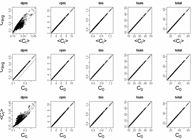
On the long term, temporal variability of the forcing variables resulted in oscillations of the 232

total SOC which size reached for some points of the standard climatic dataset 11% of the total 233

SOC, as estimated using the discrete formulation. However, over this standard climatic 234

spectrum, all methods gave similar results regarding the average SOC value at equilibrium 235

(maximum absolute error of 1%). The long term values for the different carbon compartments 236

at equilibrium were all similar but the value for the DPM compartment (Figure 1). For this 237

compartment, the effect of the temporal variability of the forcing variable (obtained by 238

comparing <Ci> to the other solutions) was important. The error caused by using RothC as

239

the discretization of the continuous formulation (see § 1.4) can be seen when comparing Cavg

240

with C0. It appears that has Cavg slightly overestimates the DPM pool compared to C0.

241

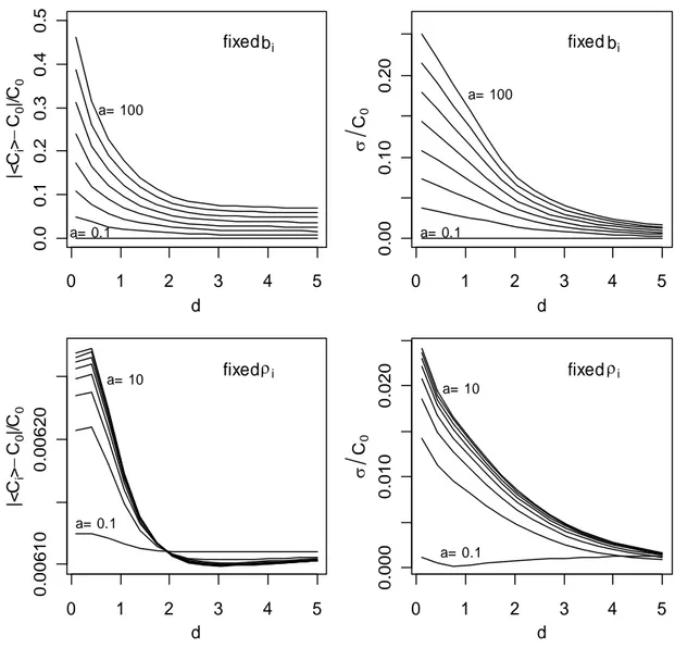
C0 became strongly biased and imprecise for extreme distributions of ρ(t) where amplitude of

242

this forcing variable was high and variability over the period was large (for a=100 and c=0.1 243

yielding maximum ρ values of 100.1, bias reached 0.5 and imprecision 0.27, Figure 2, top 244

diagrams). The imprecision and bias of C0 also depended on the amplitude and dispersion of

245

b(t) but always remained small (Figure 2, bottom diagrams). We checked (not displayed here)

246

that the bias and imprecision of C0 compared to Ci was not caused by using RothC as a

247

discretization of the continuous model but by the fact that C0 leverages the time-variability of

248

the forcing variables when Ci does not. Thus, the domains where C0 is imprecise and more

importantly biased are the domains where the time-variability of the forcing variables greatly 250

determines the behavior of the system. 251

Conclusion

252

The continuous formulation using Fourier transforms makes it possible to specify analytically 253

the forcing variables as functions of time, and then to obtain analytical solutions for the 254

mathematical formulation of the model of carbon dynamics under study. Here, we used a zero 255

order transform, which makes the forcing variables constant through time, and studied the 256

validity of such an assumption. 257

We showed in turn that such an approximation resulted in short computation times and is 258

reasonably precise (i) for the common application domain of the RothC model and (ii) in case 259

there is no concern about intra-annual variations of decomposable plant material and to a 260

smaller extent of the microbial community. If these conditions are not met, one may want to 261

use the discrete formulation or higher order Fourier transforms in order to grasp more of the 262

temporal variability of the variables. It is likely that in standard conditions, the use of average 263

agro-climatic conditions for computing steady state solutions of linear models of organic 264

matter dynamics, which is commonly found in literature on the subject (Bolker et al., 1998; 265

Baisden et al., 2003; Manzoni et al., 2004), can be legitimated. The Fourier series approach is 266

not restricted to linear models or to models taking only C dynamics into account. It could be 267

particularly relevant for non-linear systems, where assuming that forcing variable can be 268

averaged could become even more tedious than for linear systems. We also emphasize here 269

the fact that the method proposed to deal with the continuous formulation, since it essentially 270

relies on the use of Fourier series, is most suited to the modeling of periodic functions and to 271

the case where decomposition and input functions can themselves be considered as periodical. 272

The approach concerning discrete-time models was used here as a way to quickly compute the 273

long-term behavior of the discrete-time model RothC, without making any approximations 274

and thus having a larger application domain than the approach using the continuous 275

formulation. It is not likely to result in a simple analytical formulation of the equilibrium of 276

the system, because of the relative complexity of the matrix to be inversed in order to 277

compute the solution. Nevertheless, it speeds up considerably the computation compared to 278

the use of the RothC’s implementation. It can be applied to more complex systems and makes 279

it possible to take into account the full time-variability of the discrete forcing variables. There 280

might be constraints on the applicability of the discrete method, aimed at ensuring the 281

solvability of the system described in Eq.(3). Determining these constraints is out of the scope 282

of this paper but results about the Toeplitz matrices might help in this perspective. Indeed, the 283

algebraic structure of system (2) is of circulant form (or Toeplitz) and this allows the use of 284

very efficient methods for solving the eigenvalues problem we are interested in (Gray, 2006). 285

The methods proposed here to compute equilibrium solutions gave, within the RothC 286

application domain, similar results for long term SOC dynamics compared with the Fortran 287

implementation of the RothC model, while being up to 19.4 times faster. This might be 288

critical when applying the model on very large data sets, for instance those produced by 289

combining climatic, landuse and soil characteristics layers within a GIS, in order to spatially 290

compute long term SOC stocks. In addition, working at equilibrium simplifies the analysis of 291

the results as only the long-term solution is considered. Both methods are of course not 292

restricted to one-year periods and could be applied to cycles with much longer periods, for 293

instance, to crop rotations or to large climatic oscillations (with periods). It would be also 294

interesting to consider the case where, while remaining oscillatory, the forcing variables 295

exhibit a drift. This could be applied, for instance, to study the effect of climate change on 296

SOC stocks. 297

Acknowledgments

298

The authors thank David Coleman, Rothamsted Research, UK, for giving useful details about 299

the RothC implementation and the referees for their helpful comments. 300

301

Figure 1 : long-term solutions for each compartment of the model and for the total carbon content, over the 302

whole set of climatic conditions and with %clay=10%. All values are given in t.ha-1_{. First line of diagrams plots} 303

the results of the discrete formulation of RothC (<Ci>) against the results obtained with the discrete formulation

304

with constant forcing variables (Cavg). Line Two gives the results of the continuous form (C0) against Cavg and 305

line three <Ci> against C0. The plain lines drawn on the charts represent the y=x function. 306

0 1 2 3 4 5 0 .0 0 .1 0 .2 0 .3 0 .4 0 .5 d |< Ci >  C0 |/C 0 a= 0.1 a= 100 bi fixed 0 1 2 3 4 5 0 .0 0 0 .1 0 0 .2 0 d  C0 a= 0.1 a= 100 bi fixed 0 1 2 3 4 5 0 .0 0 6 1 0 0 .0 0 6 2 0 d |< Ci >  C0 |/ C0 a= 0.1 a= 10 fixed i 0 1 2 3 4 5 0 .0 0 0 0 .0 1 0 0 .0 2 0 d  C0 a= 0.1 a= 10 _i fixed 307

Figure 2 : Left hand diagrams give the precision and right hand diagrams bias of the C0estimator. Top diagrams

308

are obtained keeping the sequence of monthly inputs constant and varying dispersion and amplitude of the ρi

309

sequence. Bottom diagrams are obtained keeping the ρi sequence constant and varying dispersion and amplitude

310

of inputs over the period. a and d are the parameters used in Eq.(11). 311

312

References

313

Baisden, W.T. and Amundson, R., 2003. An analytical approach to ecosystem 314

biogeochemistry modeling. Ecological Applications, 13: 649-663. 315

Bellamy, P.H., Loveland, P.J., Bradley, R.I., Lark, R.M. and Kirk, G.J.D., 2005. Carbon 316

losses from all soils across England and Wales 1978-2003. Nature, 437: 245-248. 317

Betts, R.A., 2000. Offset of the potential carbon sink from boreal forestation by decreases in 318

surface albedo. Nature, 408: 187-190. 319

Bolinder, M.A., Angers, D.A. and Dubuc, J.P., 1997. Estimating shoot to root ratios and 320

annual carbon inputs in soils for cereal crops. Agriculture Ecosystems & Environment, 321

63: 61-66. 322

Bolker, B.M., Pacala, S.W. and Parton, W.J., 1998. Linear analysis of soil decomposition: 323

Insights from the century model. Ecological Applications, 8: 425-439. 324

Bosatta, E. and Agren, G.I., 2003. Exact solutions to the continuous-quality equation for soil 325

organic matter turnover. Journal of Theoretical Biology, 224: 97-105. 326

Cao, M.K. and Woodward, F.I., 1998. Dynamic responses of terrestrial ecosystem carbon 327

cycling to global climate change. Nature, 393: 249-252. 328

Coleman, K. and Jenkinson, D.S., 1995. ROTHC-26.3, a model for the turnover of carbon in 329

soil. Model description and users guide. Lawes Agricultural Trust, Harpenden. 330

Coleman, K., Jenkinson, D.S., Crocker, G.J., Grace, P.R., Klir, J., Korschens, M., Poulton, 331

P.R. and Richter, D.D., 1997. Simulating trends in soil organic carbon in long-term 332

experiments using RothC-26.3. Geoderma, 81: 29-44. 333

Cox, P.M., Betts, R.A., Jones, C.D., Spall, S.A. and Totterdell, I.J., 2000. Acceleration of 334

global warming due to carbon-cycle feedbacks in a coupled climate model. Nature, 335

408: 184-187. 336

Falloon, P. and Smith, P., 2002. Simulating SOC changes in long-term experiments with 337

RothC and CENTURY: model evaluation for a regional scale application. Soil Use 338

and Management, 18: 101-111. 339

Franko, U., Schramm, G., Rodionova, V., Korschens, M., Smith, P., Coleman, K., 340

Romanenkov, V. and Shevtsova, L., 2002. EuroSOMNET - a database for long-term 341

experiments on soil organic matter in Europe. Computers and Electronics in 342

Agriculture, 33: 233-239. 343

Gray, R.M., 2006. Toeplitz and Circulant Matrices: A review. Foundations and Trends in 344

Communications and Information Theory, 2: 155-239. 345

Jenkinson, D.S., Adams, D.E. and Wild, A., 1991. Model estimates of CO2 emissions from 346

soil in response to global warming. Nature, 351: 304-306. 347

Jones, C., McConnell, C., Coleman, K., Cox, P., Falloon, P., Jenkinson, D. and Powlson, D., 348

2005. Global climate change and soil carbon stocks; predictions from two contrasting 349

models for the turnover of organic carbon in soil. Global Change Biology, 11: 154-350

166. 351

Katterer, T. and Andren, O., 2001. The ICBM family of analytically solved models of soil 352

carbon, nitrogen and microbial biomass dynamics descriptions and application 353

examples. Ecological Modelling, 136: 191-207. 354

Knorr, W., Prentice, I.C., House, J.I. and Holland, E.A., 2005. Long-term sensitivity of soil 355

carbon turnover to global warming. Nature, 433: 298-301. 356

Manzoni, S., Porporato, A., D'Odorico, P., Laio, F. and Rodriguez-Iturbe, I., 2004. Soil 357

nutrient cycles as a nonlinear dynamical system. Nonlinear Processes in Geophysics, 358

11: 589-598. 359

Parshotam, A., 1996. The Rothamsted soil-carbon turnover model - Discrete to continuous 360

form. Ecological Modelling, 86: 283-289. 361

Shevtsova, L., Romanenkov, V., Sirotenko, O., Smith, P., Smith, J.U., Leech, P., Kanzyvaa, 362

S. and Rodionova, V., 2003. Effect of natural and agricultural factors on long-term 363

soil organic matter dynamics in arable soddy-podzolic soils - modeling and 364

observation. Geoderma, 116: 165-189. 365

Shirato, Y., 2005. Testing the suitability of the DNDC model for simulating long-term soil 366

organic carbon dynamics in Japanese paddy soils. Soil Science and Plant Nutrition, 367

51: 183-192. 368

Shirato, Y. and Yokozawa, M., 2005a. Applying the Rothamsted Carbon Model for long-term 369

experiments on Japanese paddy soils and modifying it by simple mining of the 370

decomposition rate. Soil Science and Plant Nutrition, 51: 405-415. 371

Shirato, Y., Paisancharoen, K., Sangtong, P., Nakviro, C., Yokozawa, M. and Matsumoto, N., 372

2005b. Testing the Rothamsted Carbon Model against data from long-term 373

experiments on upland soils in Thailand. European Journal of Soil Science, 56: 179-374

188. 375

Swinnen, J., Vanveen, J.A. and Merckx, R., 1995. Carbon Fluxes In The Rhizosphere Of 376

Winter-Wheat And Spring Barley With Conventional Vs Integrated Farming. Soil 377

Biology & Biochemistry, 27: 811-820. 378

Thornton, P.E. and Rosenbloom, N.A., 2005. Ecosystem model spin-up: Estimating steady 379

state conditions in a coupled terrestrial carbon and nitrogen cycle model. Ecological 380

Modelling, 189: 25-48. 381

Vleeshouwers, L.M. and Verhagen, A., 2002. Carbon emission and sequestration by 382

agricultural land use: a model study for Europe. Global Change Biology, 8: 519-530. 383

Yang, X., Wang, M.X., Huang, Y. and Wang, Y.S., 2002. A one-compartment model to study 384

soil carbon decomposition rate at equilibrium situation. Ecological Modelling, 151: 385

63-73. 386

387 388