HAL Id: tel-01127108
https://tel.archives-ouvertes.fr/tel-01127108
Submitted on 7 Mar 2015
HAL is a multi-disciplinary open access archive for the deposit and dissemination of sci-entific research documents, whether they are pub-lished or not. The documents may come from teaching and research institutions in France or abroad, or from public or private research centers.
L’archive ouverte pluridisciplinaire HAL, est destinée au dépôt et à la diffusion de documents scientifiques de niveau recherche, publiés ou non, émanant des établissements d’enseignement et de recherche français ou étrangers, des laboratoires publics ou privés.
Bi Li
To cite this version:
Bi Li. Tree decompositions and routing problems. Other [cs.OH]. Université Nice Sophia Antipolis, 2014. English. �NNT : 2014NICE4088�. �tel-01127108�
ET DE LA COMMUNICATION
P H D T H E S I S
to obtain the title of
Docteur en Sciences
de l’Université de Nice - Sophia Antipolis
Mention : I
NFORMATIQUEDefended by
Bi LI
Tree Decompositions and Routing Problems
COATI Project (INRIA, I3S (CNRS/UNS))
Advisors: David COUDERT
Nicolas NISSE
Defended on November 12, 2014
Jury:
Reviewers: Pascal BERTHOMÉ - LIFO (Bourges, France) Nicolas HANUSSE - CNRS (Talence, France)
-Examinators: David COUDERT - INRIA (Sophia Antipolis, France) Nicolas NISSE - INRIA (Sophia Antipolis, France) Hao LI - CNRS (Orsay, France)
Igor LITOVSKY - UNSA (Sophia Antipolis, France) Galtier JÉRÔME - Orange (Sophia Antipolis, France)
First, I am deeply indebted to my advisers David Coudert and Nicolas Nisse. Without their help, this work would not have been done. Specially, Nicolas Nisse is very patient and give me methodical and systematic guidance for doing research. I would like also to thank my coauthors Jean-Claude Bermond, Xujin Chen, Xiaodong Hu, Hervé Rivano, Karol Suchan, Joseph Yu, etc.
I dedicate this thesis to all my family, specially my grandfather, who encourages me all the time to conquer my laziness and negativeness. In particular, my mother always comforts me when I feel depressed.
I’ll always appreciate that Patricia Lachaume has helped me with all administrative problems and even personal ones for these four years. I would like to also thank so much to my dear friends Frédéric Giroire, Julio Araújo, Yaning Liu, Ana Karolinna Maia de Oliveira, Fatima Zahra Moataz and other Chinese friends in residence OXFORD. It is hard to imagine my life in France without their help and companion.
I could not mention everyone, but I would like to thank everyone in MAS-COTTE/COATI, with whom I feel so lucky to have been.
Sophia Antipolis, France November 1st, 2014
Abstract:A tree decomposition of a graph is a way to represent it as a tree by preserving some connectivity properties of the initial graph. Tree decompositions have been widely studied for their algorithmic applications, in particular using dynamic programming ap-proach. In this thesis, we study tree decompositions satisfying various constraints and design algorithms to compute them in some graph classes. We then use tree decomposi-tions or specific graph properties to solve several problems related to routing. The thesis is divided into two parts.
In the first part, we study tree decompositions satisfying some properties. In Chapter 2, we investigate minimum size tree decompositions, i.e., with minimum number of bags. Given a fixed k ≥ 4, we prove it is NP-hard to compute a minimum size decomposition with width at most k in the class of graphs with treewidth at least 4. We design polynomial time algorithms to compute minimum size tree decompositions in some classes of graphs with treewidth at most 3 (including trees). Part of these results will be presented in ICGT 2014.
In Chapter 3, we study the chordality (longest induced cycle) of graphs and introduce the notion of good tree decomposition (where each bag must satisfy some particular struc-ture). Precisely, we study the Cops and Robber games in graphs with no long induced cycles. Our main result is the design of a polynomial-time algorithm that either returns an induced cycle of length at least k + 1 of a graph G or compute a k-good tree decomposition of G. These results have been published in ICALP 2012 and Algorithmica.
In the second part of the thesis, we focus on routing problems. In Chapter 4, we design a compact routing scheme that achieves good performance in the class of graphs admitting k-good tree decompositions.
In Chapter 5, we consider the prize collecting Steiner tree problem (a generalization of the Steiner-tree problem with weighted nodes and edges). We design two risk models of the problem when the weights are given as intervals. In these models, we design polynomial-time algorithms for graphs with small treewidth. These results have been published in AAIM 2010 and the journal Acta Mathematicae Applicatae Sinica.
Finally, in Chapter 6, we consider the gathering problem in grids and in presence of in-terferences. We design approximation algorithms (up to small additive constants depending on the interferences) for solving this problem. This work is in revision for TCS.
Keywords:Tree Decomposition, Compact Routing Scheme, Prize Collecting Steiner Tree, Gathering.
Résumé :
Une décomposition arborescente d’un graphe est une manière de le représenter sous forme d’un arbre (dont les sommets sont appelés ’sac’), en préservant des propriétés de connexité. Les décompositions arborescentes ont été beaucoup étudiées pour leurs applica-tions algorithmiques qui utilisent, en particulier, la programmation dynamique. Dans cette thèse, nous étudions les décompositions arborescentes qui satisfont certaines contraintes supplémentaires et nous proposons des algorithmes pour les calculer dans certaines classes de graphes. Finalement, nous résolvons des problèmes liés au routage en utilisant ces dé-compositions ainsi que des propriétés structurelles des graphes. Cette thèse est divisée en deux parties.
Dans la première partie, nous étudions les décompositions arborescentes satisfaisant des propriétés spécifiques. Dans le Chapitre 2, nous étudions les décompositions de taille minimum, c’est-à-dire avec un nombre minimum de sacs. Etant donné une entier k ≥ 4 fixé, nous prouvons que le problème de calculer une décomposition arborescente de largeur au plus k et de taille minimum est NP-complet dans les graphes de largeur arborescente au plus 4. Nous décrivons ensuite des algorithmes qui calculent des décompositions de taille minimum dans certaines classes de graphes de largeur arborescente au plus 3 (en particulier dans les arbres). Ces résultats ont été présentés au workshop international ICGT 2014.
Dans le Chapitre 3, nous étudions la cordalité (plus long cycle induit) des graphes et nous introduisons la notion de k-good décomposition arborescente (où chaque sac doit ad-mettre une structure particulière). Nous étudions tout d’abord les jeux de Gendarmes et Voleur dans les graphes sans long cycle induit. Notre résultat principal est un algorithme polynomial qui, étant donné un graphe G, soit trouve un cycle induit de longueur au moins k+1, ou calcule une k-good décomposition de G. Ces résultats ont été publiés à la con-férence internationale ICALP’12 et dans la revue internationale Algorithmica.
Dans la seconde partie de la thèse, nous nous concentrons sur des problèmes de routage. Dans le Chapitre 4, nous concevons un algorithme de routage compact qui a de très bonnes performances dans les graphes qui admettent une k-good décomposition.
Dans le Chapitre 5, nous considérons le problème du "Price Collecting Steiner Tree". Nous proposons 2 modèles de risque pour ce problème (lorsque les poids des sommets et coûts des arêtes sont donnés sous forme d’intervalles). Pour ces deux modèles, nous proposons des algorithmes polynomiaux qui résolvent ces problèmes dans les graphes de petite largeur arborescente. Ces résultats ont été publiés dans AAIM 2010 et dans la revue Acta Mathematicae Applicatae Sinica.
Finalement, dans le Chapitre 6, nous considérons le problème de collecte d’information dans les réseaux en grille et en présence d’interférences. Nous proposons des algorithmes d’approximation (à une petite constante additive près) pour résoudre ce problème. Ce travail est en révision pour la revue internationale TCS.
1 Introduction 1
I Tree Decomposition 17
2 Minimum Size Tree Decomposition 19
2.1 Introduction . . . 19
2.2 NP-hardness in the class of bounded treewidth graphs . . . 20
2.3 Notations and preliminaries . . . 23
2.3.1 Notations . . . 23
2.3.2 General approach . . . 25
2.4 Graphs with treewidth at most 2 . . . 26
2.5 Minimum-size tree-decompositions of width at most 3 . . . 34
2.5.1 computation of s3in trees . . . 34
2.5.2 Computation of s3in 2-connected outerplanar graphs . . . 41
2.6 Perspective . . . 46
3 k-Good Tree Decomposition 49 3.1 Introduction . . . 50
3.1.1 Related Work . . . 51
3.1.2 Notations and Definitions . . . 52
3.2 A detour through Cops and Robber games . . . 53
3.3 Structured Tree-decomposition . . . 55
3.4 Recognition and Chordality of Planar k-Super-Caterpillars . . . 59
3.4.1 NP-completeness of the recognition of planar k-super-caterpillars . 59 3.4.2 Chordality of planar k-super-caterpillars . . . 60
3.5 Perspectives . . . 72
II Routing Problems 73 4 Compact Routing Scheme for k-Good Tree Decomposable Graphs 75 4.1 Introduction . . . 75
4.1.1 Related Work . . . 76
4.2 Model And Data Structures . . . 77
4.2.1 Routing In Trees [FG01] . . . 78
4.2.2 Data Structures . . . 78
4.3 Compact Routing algorithm in k-good tree-decomposable graphs . . . 79
4.4 Performance of the routing scheme . . . 80
5 Prize Collecting Steiner Tree Problem on Partial 2-Trees 83
5.1 Introduction . . . 84
5.2 Dynamic Programming for PCST on Partial 2-Trees . . . 87
5.2.1 Preliminary Definitions and Notations . . . 87
5.2.2 Dynamic Programming . . . 91
5.3 Risk Models for PCST Problem with Interval Data . . . 95
5.3.1 PCST Problem under Min-Max Risk Model . . . 95
5.3.2 PCST Problem under Min-Sum Risk Model . . . 100
5.3.3 Discussion . . . 109
5.4 Perspectives . . . 110
6 Data Gathering and Personalized Broadcasting in Radio Grids 111 6.1 Introduction . . . 112
6.1.1 Problem, model and assumptions . . . 112
6.1.2 Related Work . . . 114
6.1.3 Main results . . . 114
6.2 Notations and Lower bound . . . 115
6.3 Basic instance: dI= 0, open-grid, and BS in the corner . . . 118
6.3.1 Basic schemes . . . 118
6.3.2 Interference of messages . . . 119
6.3.3 Basic lemmas . . . 120
6.3.4 Makespan can be approximated up to additive constant 2 . . . 121
6.3.5 Makespan can be approximated up to additive constant 1 . . . 124
6.4 Case dI= 0; general grid, and BS in the corner . . . 132
6.5 dI-Open Grid when dI∈ {1, 2} . . . 136
6.5.1 Lower bounds . . . 136
6.5.2 Routing with ε-detours . . . 138
6.5.3 General-scheme dI= 1. . . 141
6.5.4 General-scheme dI= 2. . . 143
6.6 Personalized Broadcasting in Grid with Arbitrary Base Station . . . 145
6.7 Perspective . . . 147
Introduction
How do people keep up to date with the happenings around the world? How do people keep in touch with friends all over the world? How do people find the information they need... Most people will answer by the Internet. It goes without saying that Internet is very important in our life.
One of the main roles of the Internet, also all kinds of communication network, e.g. transportation network, social network, is to transmit information. Then a fundamental task is to route the information between any pairs of its clients, which can be computers, stations or people, that is to find paths in the network.
How to route the information efficiently, i.e., to find a desired path from the origin to the destination quickly? Everyone knows how to go home after work everyday, because they know the way from home to work. But imagine that someone is going to visit a new city. Without a GPS or a map in their hand, they will spend a long time to find their way. We see that the map, which shows the topology of the network (city), is important to do efficient routing. It is not so difficult to get a map of a city, because we can record all the buildings and all the roads in the map. However, what about getting a map of the Internet network, Facebook, Twitter, etc.? So far, there are more than 65,000 Autonomous Systems (AS) in the Internet [fIDAC]. Furthermore, according to [Cis14], over half a billion (526 million) mobile devices and connections were added and global mobile data traffic grew by 81% in 2013. There were nearly 22 million wearable devices1 in 2013 generating 1.7 petabytes of monthly traffic. The telecommunication networks are not only becoming larger and larger but also more and more dynamic. All this brings difficulties in getting a map, i.e. in knowing the global topology of the network. It is almost impossible to get it because the Internet is changing all the time with many new devices connecting to the Internet and at the same time many devices disconnecting from the Internet.
How does the Internet route nowadays? Routing in the Internet is mainly guided by Border Gateway Protocol (BGP). Simply speaking, in BGP, every router stores a path to any other router in the Internet. Since the Internet is changing all the time, the paths stored in each router is also changing accordingly. Moreover, every router needs a big memory to store the paths since there are huge numbers of routers in the Internet. Because of the growth of the Internet, BGP may not work any more in the future. It is important to improve BGP and also explore new protocols for routing in the Internet.
1The so called wearable devices are devices that can be worn on a person, which have the capability to
connect and communicate to the network either directly through embedded cellular connectivity or through another device (primarily a smartphone) using Wi-Fi, Bluetooth or another technology, such as smart watches, smart glasses, health and fitness trackers, health monitors, wearable scanners, navigation devices, smart cloth-ing, and so forth [Cis14].
A lot of research is dedicated to implement experiments to measure some properties of large-scale networks, e.g. the Internet network. There are already many well known struc-tural properties of the large-scale networks, such as logarithmic diameter (the diameter of the network is much smaller than the number of clients), power-law degree distribution (there are few clients connected with many other clients) and high clustering coefficient (two clients connected with another one common client has big probability to be con-nected) [BA99, AJB99, SFFF03, FFF99]. Traditionally, a network can be modeled by a graph with the vertex set of all the clients and the edge set of possible connections between two clients. Using some graph libraries or network simulators, e.g. Grph, DRMsim, NS simulator, researchers and engineers are able to generate graph models satisfying some of the above structural properties of the large-scale networks. Moreover, many efficient routing algorithms are designed for these graph models [KFY04, CSTW12]. There is big probability that these algorithms work also well in the real life large-scale networks, be-cause these graph models satisfy the same properties. So it is interesting to design efficient algorithms for graph models of large-scale networks. To design efficient algorithms for any graph, it is helpful to take advantage of some particular structural properties of the graph. The main motivation of my thesis is to explore the structural properties of graphs, which may be used for algorithmic purposes.
One of the simplest classes of (undirected) graphs is the class of trees, connected acyclic graphs. Many difficult (NP-complete) problems become easy (polynomially solv-able) in the class of trees, see e.g. [DN66, CGH75]. It is conceivable that many prob-lems should be also easy in a class of graphs ’close’ to trees. But how to define that a graph is ’close’ to a tree? This question leads to the main topic of my PhD thesis, tree decomposition, which is a way to study likeness of a graph. Roughly speaking, a tree-decompositionof a graph maps each vertex of the graph to a subtree of the decomposition treein a way that the subtrees assigned to the adjacent vertices intersect [RS86b, Bod98]. Such decompositions play an important role in design of efficient algorithms. Let us see some definitions before presenting its algorithmic applications.
Definitions and Notations
In this section, we give some basic definitions used in this thesis. All the definitions in this section can be found in [BM08].
For any two sets A and B, if any element in B in contained in A, we say that B is a subset of A, denoted as B ⊆ A; if B ⊆ A and B 6= A then we say B is a proper subset of A, denoted as B ⊂ A. Let G = (V, E) be any undirected simple graph. For any two adjacent vertices u, v ∈ V , we denote the edge as uv. Any graph G0 = (V0, E0) with V0 ⊆ V and E0⊆ {uv ∈ E : u, v ∈ V0} is a subgraph of G; moreover G0is an induced subgraph of G, or subgraph induced by V0, denoted as G[V0], if E0= {uv ∈ E : u, v ∈ V0}. For a set M ⊆ V ∪ E, we denote by G \ M the subgraph (V \ M, (E \ M) \ {uv : u ∈ M or v ∈ M}) of G. For any subgraph H of G, denoted as H ⊆ G, we use V (H) and E(H) to denote the vertex and edge set of H, respectively. A graph is connected if there is a path between any two vertices in it. A graph is disconnected if it is not connected. A connected component of a graph G is
a maximal connected subgraph of G.
A graph is complete if any of its two vertices are adjacent. We denote by Kna complete
n-vertex-graph. Given a graph G, a subgraph K of G is a clique if K is complete. A graph G= (V, E) is bipartite if there exist two disjoint subsets A, B ⊆ V such that V = A ∪ B and each edge in E is incident to a vertex in A and the other one in B; moreover G is a complete bipartitegraph if each vertex in A and each vertex in B are adjacent. We denote the complete bipartite graph G by K|A|,|B|. A graph is planar if it can be embedded in the
plane, i.e., it can be drawn on the plane in such a way that its edges intersect only at their endpoints. In other words, it can be drawn in such a way that no edges cross each other. Such a drawing is called a planar embedding of the graph. A planar graph is outerplanar if it has a planar embedding such that all its vertices belong to the unbounded face.
Given a graph G = (V, E), the distance between two vertices u, v ∈ V in G is the length, i.e., the number of edges, of a shortest path between them in G. For any vertex v ∈ V , the open neighborhoodof v is defined as NG(v) = {u : uv ∈ E}; the closed neighborhood of
v is defined as NG[v] = NG(v) ∪ {v}. When the graph is clear from the context, without
confusion we use N(v) or N[v] simply. The degree of a vertex v in G is |NG(v)|. We denote
by ∆ the maximum degree over all vertices in G. A subset D ⊆ V (G) is a dominating set of the graph G if any vertex not in D is adjacent to some vertices in D.
Tree Decomposition
Definition 1. Given a graph G = (V, E), a tree decomposition (T,X) of G consists of a tree T and a familyX = {Xt : t ∈ V (T )} of subsets of V , called bags, such that:
• ∪t∈V (T )Xt = V ;
• for any edge e = uv ∈ E, there exists a node t ∈ V (T ) such that the bag Xt contains
both u and v;
• for any vertex v ∈ V , the nodes in {t ∈ V (T ) : v ∈ Xt} induces a subtree of T .
The width of (T,X) is maxt∈V (T )|Xt| − 1, i.e. the maximum size of a bag minus one.
The treewidth2 of G, denote by tw(G), is the minimum width among all the tree decom-positions of G [RS86b]. For each bag Xt, the diameter of Xt, denoted by diam(Xt), is
the maximum distance in G between any two vertices in Xt. The length of (T,X) is
maxt∈V (T )diam(Xt), i.e. the maximum diameter of all bags in X. The treelength of G,
denote by tl(G), is the minimum length among all the tree decompositions of G [DG07]. Moreover, (T,X) is a path decomposition of G if T is a path. The pathwidth of G, denote by pw(G), is the minimum width among all the path decompositions of G [RS83].
Given a tree decomposition (T,X = {Xt : t ∈ V }) of G, without confusion, we identify
the bag Xt ∈X and the node t ∈ V(T).
It is well-known that forests, union of disjoint trees, are exactly the class of graphs of treewidth at most 1.
2Note that, while the term treewidth has been defined by Robertson and Seymour in their work on Graph
Tree decomposition has been first introduced by Robertson and Seymour in the Graph Minor theory[RS86b]. Let us give some basic definitions about graph minor.
Given an edge uv ∈ E(G), the edge contraction of uv in G, is to identify vertices u and v in G and removing all loops and duplicate edges. The obtained graph is denoted by G/{uv}. A graph H is a contraction of a graph G if H can be obtained by a sequence of edge contractions from G. Particularly, we say that G is also a contraction of G. A minor of a graph G is a contraction of a subgraph of G. (Note that G is also a subgraph of G.) Given an n-vertex-graph G, for every fixed graph H there exists an O(n3) algorithm testing whether H is a minor of G, where the big O notation hides a constant that depends superexponentially on |V (H)|; while, if G is given with a tree decomposition of bounded treewidth, then it can be tested in linear (but exponential in |V (H)|) time whether H is a minor of G [RS95]. Kawarabayashi et. al improved their time complexity to O(n2) (for general graph G) in [iKKR12].
The famous Wagner’s theorem says that a graph is planar if and only if it does not contain K5and K3,3 as a minor. It is well-known that a graph is outerplanar if and only if
it does not contain K4and K2,3as a minor. A graph is a partial 2-tree if it has treewidth at
most 2. Wald and Colbourn proved that:
Theorem 1. [WC83] A graph is a partial 2-tree if and only if it does not contain K4as a
minor.
In Fig. 1.1, we see the clear hierarchy of the classes of forest, outerplanar graphs, partial 2-trees and planar graphs.
A class of graphsC is minor-closed if any minor of any graph in C is also a member of C. Given a minor-closed class of graphs C, denote its complementary as ¯C, i.e. the set of graphs not inC. A graph F ∈ ¯C is a forbidden minor of C if F is minimal in ¯C, i.e. no other graphs in ¯C is a minor of F, equivalently any minor of F is in C. So Theorem 1 says K4
is the only forbidden minor of the class of partial 2-trees. Robertson and Seymour proved that:
Theorem 2. [Graph Minor Theorem] Every minor-closed class of graphs has finite num-ber of forbidden minors [RS04].
Planar graphs
Partial 2-trees Outerplanar graphs
Forests
Figure 1.1: The hierarchy of the classes of forest, outerplanar graphs, partial 2-trees and planar graphs.
Tree decompositions are also used in parameterized complexity theory. A parameter is a function mapping graphs to nonnegative integers, e.g. chordality, treewidth. A pa-rameterized problem, taking as parameter a fixed nonnegative integer k and as input an
instance I, is Fixed Parameter Tractable (FPT) if there is an algorithm that solves it in time f(k)nO(1)I , where nIis the size of the instance and f is a function depending only on k. We
are going to see later that many parameterized problems are FPT, which takes as input a graph G and as parameter the treewidth of G.
Plenty of work is devoted to compute the treewidth of a given graph. One of the well-known exact algorithms for treewidth computation is given by Fomin et al. [FKTV08], which is base on minimal triangulation of a graph. We present the related definitions in the following.
A graph G is k-chordal for an integer k if there is no induced cycle, cycle without chords, longer than k. The chordality of a graph G is the minimum k such that G is k-chordal. In particular, a 3-chordal graph G is also called chordal graph. Given a graph G= (V, E), a graph G+= (V, E ∪ F) is a triangulation of G if G+is chordal; moreover G+ is a minimal triangulation of G if for any proper subset F0⊂ F, the graph H = (V, E ∪ F0) is not chordal. That is to say that a minimal triangulation of G is obtained by adding a minimal set of edges to G to make it chordal. There is a n2.376time algorithm for finding a minimal triangulation of an n-graph in [Mez11].
Chordal graphs have many different characterizations, see e.g. a survey [Heg06]. A clique treeof a graph G is a tree decomposition of G such that the vertices in each bag of the tree decomposition induces a clique in G. A graph G is chordal if and only if it has a clique tree [Gav74, Bun74].
Given a graph G and a tree decomposition (T,X) of width tw(G), construct a graph G+by adding an edge uv in G if there exists a bag in (T,X) containing both u and v. Then (T,X) is a clique tree of G+. So G+ is a chordal graph. This gives hints to the following well known fact: G has treewidth at most k if and only if G has a minimal triangulation with maximum clique of size at most k+ 1.
So the treewidth of a graph is closely related to the cliques in its minimal triangulations. Given a graph G = (V, E), a potential maximal clique is a set of vertices in G which induces a maximal clique in some minimal triangulation of G.
Given a graph G = (V, E), two vertices u, v ∈ V in a same connected component of G and a subset S ⊆ V \ {u, v}, we say that S separates u and v, if u and v are in different connected component of the subgraph G \ S; S is a separator of G if there exist u, v ∈ V such that S separates u and v. Moreover S ⊂ V is a minimal separator if there exist u, v ∈ V such that S separates u and v but none of its proper subset S0⊂ S separates u and v. In general, for any three subsets U,W, S ⊆ V , we say that S separates U and W if each path between any vertex u ∈ U and any vertex w ∈ W contains a vertex in S. Bouchitté and Todinca proved that treewidth can be computed in polynomial time in the class of graphs, which have polynomial number of minimal separators [BT02].
Treewidth Computations
In this section, we present some previous work focusing on the treewidth computation. Many NP-hard problems in general graphs have been shown to be polynomially sol-vable in the class of graphs with bounded treewidth. Particularly, the famous Courcelle’s
theorem states that all problems expressible in monadic second order logic3can be solved in linear time in the class of graphs with bounded treewidth [Cou90]. It means that the algorithm is linear time in the size of a given graph but maybe exponential in its treewidth. Due to the important role of treewidth, the problem ’Given an n-vertex-graph G = (V, E) and an integer k, is the treewidth of G at most k?’ received much attention.
This problem has been proved to be NP-complete by Arnborg et al. in [ACP87]. Ad-ditionally, they showed that the problem is solvable in O(nk+2) time for a fixed k. Later, Robertson and Seymour proved that there exists an O(33kn2) time algorithm for this prob-lem [RS95]. Their algorithm consists of two steps: first, apply an O(33kn2) algorithm that either decides that the treewidth of G is bigger than k, or computes a tree decomposition of Gwith width at most 4k + 3; if the first step outputs a tree decomposition of G with width at most 4k + 3, then implement the second step: Since the class of graphs with treewidth at most k is minor-closed (see the reason in the subsection Graph Minor), it has a finite number of forbidden minors. Given G with a tree decomposition of width at most 4k + 3, they check in linear time whether G has treewidth at most k by testing whether G has some of those forbidden minors as minors. Note that the second step is non-constructive because the forbidden minors are known to be finite but not listed. The time complexity is dominated by the first step. (Actually, the results in [RS95] are presented in terms of branchwidth, which is equivalent to treewidth up to a constant factor [RS91]. So this is an unimportant technical difference.)
Plenty of work is devoted to improve the time complexity of the two steps in this algo-rithm. Based on the notion of ’balanced separators’, Lagergren [Lag96] and Reed [Ree92] can implement the first step in kO(k)nlog2nand kO(k)nlog n time respectively. Bodlaender made it be linear time and the total time complexity was kO(k3)n, by reducing the problem for G in linear time to a problem on a smaller graph, which is a minor of G [Bod96]. On the other hand, the second step can be improved without using graph minors; and there exist linear time (single exponential in k) constructive algorithms for deciding whether G has treewidth at most k if G is given with a tree decomposition of width O(k)(see e.g. [BK91, LA91]).
Note that given a graph G of treewidth k, the first step of the algorithm outputs a tree de-composition of G with width at most 4k + 3. Then it is a 4-approximation for the treewidth. All the algorithms above have time complexities either not linear in n or not single expo-nential in k. Recently, Bodlaender et al. has given the first algorithm of time complexity linear in n and single-exponential in k [BDD+13]. More precisely, given a graph G and an integer k, their algorithm, in time 2O(k)n, either outputs that the treewidth of G is bigger
3Monadic second-order formulasin the language of graphs are built up from:
• atomic formulas E(x, y), x = y and X(x) (for set variable X and individual variables x, y) by using the usual Boolean connectives ¬ (negation), ∧ (conjunction), ∨ (disjunction), → (implication), and ↔ (equivalence) and
• existential quantification ∃x, ∃X and universal quantification ∀x, ∀X over individual variables and set variables.
Individual variables range over vertices of a graph and set variables are interpreted by sets of vertices. The atomic formula E(x, y) expresses adjacency, the formula x = y expresses quality and X (x) means that the vertex xis contained in the set X .
that k, or constructs a tree decomposition of G of width at most 5k + 4. So for a graph with treewidth at most k, there is a 5-approximation algorithm for finding its treewidth in time 2O(k)n. Polynomial time approximation (but not constant ratio) algorithms for treewidth can be found in [Ami10, FHL08].
In [BB05, BK07, BK10, BK11], several heuristic algorithms are presented for comput-ing lower or upper bounds of the treewidth of a given graph.
There are also exact (exponential) algorithms for finding the treewidth of a given graph. In [BT01], Bouchitté and Todinca gave an algorithm for computing the treewidth of a given graph in polynomial time in the number of potential maximal cliques. In [BT02], they listed all potential maximal cliques of a graph in polynomial time in the number of minimal separators of the graph. So if we list all the minimal separators or all the potential maximal cliques of a given graph, then the treewidth can be computed. Based on this idea, Fomin et al. gave an O(1.8899n) time algorithm to find the treewidth of an n-vertex-graph in [FKTV08]. Fomin and Villanger presented an O(1.7549n) time algorithm in [FV12].
Algorithmic Applications of Tree Decompositions
Tree decompositions have been used in many areas (see a survey e.g. [Bod93]). We present in this section some of their algorithmic applications in graph problems.
Graph Minors
In this subsection, we briefly introduce the role of tree decomposition in proving the Graph Minor Theorem[RS86b].
First let us show that the class of graphs with bounded treewidth are minor-closed. Given a graph G = (V, E), let (T,X) be a tree decomposition of width k of G. Then (T,X) is also a tree decomposition of any subgraph obtained by deleting any edges of G; for any vertex v ∈ V , deleting v in all bags of (T,X), (T,X) becomes a tree decomposition of width at most k of the subgraph G \ {v} of G; for any edge uv ∈ E, identifying u and v in all bags of (T,X), (T,X) becomes a tree decomposition of width at most k of the contraction graph G/{uv} of G. So the treewidth of a minor of the graph G is at most the treewidth of G.
The Graph Minor Theorem, see in Theorem 2, is proved by Robertson and Seymour in a series of twenty papers spanning over 500 pages from 1983 to 2004. In particular, they proved that the set of graphs with bounded treewidth has a finite set of forbidden minors [RS90]; and that the class of graphs having a fixed planar graph as a forbidden minor has bounded treewidth [RS84, RS86a]. These two facts play an important role in the proof of the Graph Minor theorem. Particularly, the grid minor theorem is involved in the proofs, which says that any graph either has bounded treewidth or has a large grid as minor [RST94]. More precisely, we display the related results on grid minor theorem in the following.
Theorem 3. [grid minor theorem] Let G be a graph with treewidth at least k, then G contains r× r-grid as a minor, where r ≥ f (k) for some function f :
• f (k) = Ω(kδ) for a fixed constant δ > 0 [CC13];
• if G is H-minor free, then f (k) = Ω(k) [DH08b, iKK12].
There exists graph with treewidth at least k but no O(pk/ log k) × O(pk/ log k) grid as a minor [RST94].
We are going to see later that the grid minor theorem is one of the bases of the bidi-mensionality theory.
Dynamic programming
In this subsection, we present dynamic programming, the main technique for efficiently solving problems in bounded treewidth graphs.
As mentioned before, many NP-hard problems in general graphs are polynomially sol-vable in the class of graphs with bounded treewidth, e.g. maximum independent set prob-lem, minimum dominating set probprob-lem, coloring probprob-lem, etc. Given an n-vertex-graph G these problems can be solved in ctw(G)nO(1) time for a constant c, see e.g. [AP89, TaP97]. Such algorithms generally proceed by dynamic programming.
Given an n-vertex-graph G and a tree decomposition (T,X) of width tw(G), let bag Xr be the root of T . Consider e.g. the maximum independent set problem, in which it is
required to find a maximum set of vertices in G that are pairwise non-adjacent. Each leaf bag Xf induces a subgraph of G with at most tw(G) + 1 vertices. Let Xp be the parent
bag of Xf in T . Consider the intersection set S = Xf ∩ Xp. The set S separates Xf\ S and
V(G) \ Xf. For each independent set I ⊆ S in the induced subgraph G[Xf], find a ’partial
optimal solution’ MI, which is a maximum independent set in G[Xf] and satisfies MI∩S = I.
This can be done in O(2tw(G)) time because |Xf| ≤ tw(G) + 1. For each non-leaf-bag Xiin
(T,X), let Gibe the subgraph of G induced by vertices in Xiand its descendants in T . For
all children Xjs of Xiin T , we combine the ’partial optimal solutions’ of the subgraphs Gjs
to get ’partial optimal solutions’ for the subgraph Gi, until we get an optimal solution for
the graph Gr= G. More precisely, consider each independent set Y ⊆ Xi in the subgraph
Gi. Let Xjbe a child of Xiin T . Denote Si j= Xi∩ Xj. Then a maximum independent set MY
in Gi s.t. MY∩ Xi= Y can be obtained by the union of Y and the ’partial optimal solution’
containing Si j∩Y for each child Xj of Xi in the subgarph Gj. Let Spbe the intersection of
Xiand its parent bag. Among all MY with the same Y ∩ Sp, record one MY with maximum
size. This can be done in O(2tw(G)n) because there are at most 2tw(G)independent sets in Xiand Xi has at most n − 1 children. So it takes O(2tw(G)n2) time totally.
The key point of the above dynamic programming algorithm is that the intersection of two adjacent bags in the tree decomposition is a separator of the graph. Moreover, for the locally checkable problem, e.g. maximum independent set problem, it is sufficient to record an optimal partial solution respective to each subset of this intersection. On the other hand, the problems involving global constraints, e.g. the connectivity problem, may require to record an optimal partial solution respective to each ordered subset of this intersection. Generally it leads to running time tw(G)tw(G)nO(1).
It was a long-standing challenge to find algorithms for the ’global constraints’ prob-lem with time complexity single exponential on the treewidth. Fortunately, combin-ing the dynamic programmcombin-ing with other techniques, such as sphere cut decomposition, Catalan number, matrix rank and determinants, the connectivity problem can also be solved in time single exponential in the treewidth, i.e. 2O(tw(G))nO(1). Please see details in [DPBF10, ST10, DFT12, BCKN13].
From the time complexity of the above algorithms (2O(tw(G))nO(1)or tw(G)tw(G)nO(1)), we get that all the problems above are FPT with parameter treewidth of a graph. We are going to see in the next subsection that some parameterized problems with a parameter k are FPT sub-exponential (i.e. 2o(k)nO(1)) solvable by using bidimensionality theory.
Bidimensionality Theory
In this subsection, we present some previous work on bidimensionality theory, which com-bines the grid minor theorem and dynamic programming technique in the previous subsec-tions.
The Bidimensionality theory has been introduced and developed in a series of papers, see in a survey [DH08a] and references in it. A parameter P is (minor) bidimensional if
(i) there exists a function g such that the parameter P is at least g(r) in an r × r-grid Gr×r; and
(ii) it does not increase when taking minors, i.e. for any graph G and its minor H, P(H) ≤ P(G).
Consider a decision problem associated with a parameter P, for a given graph G and a nonnegative integer p, asking whether P(G) ≤ p. Let P be a (g(r)-) bidimensional param-eter. Let f be the same function as in Theorem 3, if the treewidth of G is Ω( f−1g−1(p)), then G has a grid Gg−1(p)×g−1(p) as a minor. So P(G) ≥ P(Gg−1(p)×g−1(p)) > p; otherwise, the treewidth of G is bounded by a function of p. If we can find a tree decomposition of bounded width of G, then the problem can be solved by using dynamic programming pre-sented in Section 1. So to solve this problem it is sufficient to answer : given a graph G and an integer k > 0 (Ω( f−1g−1(p))), is the treewidth of G at most k? And if yes, find a tree de-composition of width O(k) of G. We have seen that this can be done in time (2O(k)n) in the previous section [BDD+13]. So when f−1g−1(p) = o(p), we get an FPT sub-exponential time algorithm.
Moreover, this technique has been extended for parameters with less constrained prop-erties, called contraction-bidimensionality [DFHT05, DH08a]. The main differences are that contraction-bidimensionality parameter does not increasing when taking contraction instead of minor, and it is ’large’ (i.e. at least g(r)) in a ’grid like’ graph instead of grid. But the grid like graphs are only defined for the classes of planar graphs, bounded genus graphs and apex-minor-free graphs. For instance, a planar grid like graph is an r × r grid partially triangulated by additional edges that preserve planarity. For more details please see in [DFHT05, DH08a].
In particular, the parameter chordality of a graph is contraction-bidimensional. The decision problem associated with the chordality, for a given graph G and a nonnegative
integer p, asks whether the chordality of G is at most p. We are going to show that this problem is FPT (and subexponential on the parameter chordality) in the class of planar graphs in Chapter 3.
Other parameters related with tree decompositions
In this section, we present some limitations of the application of tree decompositions of bounded width. Then we introduce some other parameters related to tree decompositions, which are used for efficiently solving some graph problems.
We have seen that tree decompositions of bounded width are the corner-stone for solv-ing efficiently many graph problems. However, the algorithms presented above for com-puting a tree decomposition of bounded width of a given graph are mainly of theoretical importance due to the hidden huge constants or multiple-exponential functions of the pa-rameters. Only for the class of graphs of treewidth at most 4, there are practical linear algorithms for finding an optimal tree decomposition by a finite set of reduction rules, which reduces a graph to an empty graph if and only if the graph has treewidth at most 4 [AP86, MT91, San96]. Indeed, for any nonnegative integer k, there is a finite set of reduc-tion rules for the class of graphs of treewidth at most k [ACPS93, BF96]. But for k > 4, the algorithms based on reduction rules may require big (exponential on k) memories [Bod07]. The lack of practical algorithm for treewidth computation is still a bottleneck of its appli-cations in practice. Moreover, unless P = NP there is no polynomial time algorithm that given a graph G computes a tree decomposition of width within an additive constant of tw(G) [BGHK91]. Assuming the Small Set Expansion Conjecture4, the treewidth, also the pathwidth, are NP-hard to approximate within a constant factor [APW12]. In addition, the complexity of the computing the treewidth of planar graphs is still a longstanding open problem.
On the other hand, there also exist problems, which remain hard for the class of graphs with constant bounded treewidth, but become polynomially solvable on some class of graphs with unbounded treewidth. For instance, the bandwidth problem5 is NP-complete even for trees [GGJK78, Mon86]. But this problem is polynomially solvable in the class of interval graphs [KV90]. A graph is an interval graph if every vertex in the graph can be associated with an interval in the real line so that two vertices are adjacent in the graph if and only if the two corresponding intervals intersect.
4Let G = (V, E) be an undirected d-regular graph, i.e. every vertex has degree d in G. For a set S ⊆ V of
vertices, the normalized edge expansion of S is ΦG(S) ≡|E(S,V \S)|d|S| , where E(S,V \ S) = {uv ∈ E : u ∈ S, v ∈
V\ S}. The Small Set Expansion Problem with parameter η and δ , denoted by SSE(η, δ ), distinguish two cases:
Yes there exists an S ⊆ V with |S| = δ |V | and ΦG(S) ≤ η;
No For any subset S ⊆ V with |S| = δ |V | it holds that ΦG(S) ≥ 1 − eta.
The Small Set Expansion Conjecture says that For any η > 0, there is a δ > 0 such that SSE(η, δ ) is NP-hard.
5Given an n-vertex graph, a linear arrangement is a numbering of the vertices from 1 to n (which can be
viewed as a layout of the graph vertices on a line) and its bandwidth is the maximum difference in numbers given to the endpoints of an edge (the maximum stretch of an edge on the line). The (minimum) bandwidth problem asks for a linear arrangement of minimum bandwidth.
A clique path of a graph G is a path decomposition of G such that each of its bag induces a clique in G. A graph G is interval if and only if it has a clique path. So the class of interval graphs has unbounded treewidth. The algorithm in [KV90] for solving the bandwidth problem in interval graphs used the clique paths of interval graphs, which is actually a special path decomposition, and also a tree decomposition satisfying some structure properties. The complexity of computing the pathwidth is NP-complete even in the class of chordal graphs [Gus93]. We do not know any good approximation algorithms for computing pathwidth in chordal graphs. It is an on-going work not included in this thesis.
In [DG07] Dourisboure and Gavoille introduce the treelength of a graph, which studies the structures inside each bag of the tree decomposition, the maximum diameter of each bag. Note that chordal graphs are exactly graphs of treelength 1. It is NP-complete to decide wether a given graph has treelength at most any fixed k ≥ 2 [Lok10], but it has an easy linear time 3-approximation algorithm [DG07]. The bounded treelength graphs are proved to admit compact routing schemes [Dou05] and sparse additive spanners [DG04]. Recently, Dragan and Köhler introduced in [DK11] another parameter related with tree-length, named treebreadth, which is the minimum of the maximum radius6of all the bags among all the tree decompositions. Treebreadth is proved to be useful for tree spanner problem[DK11, DAA13].
Motivated by application in parallel and dynamic graph algorithm, Bodlaender and Hagerup investigated the tradeoff between the width and the diameter of tree decompo-sitions [BH98]. Note that here the diameter is not the diameter of the bags in the tree decompositions, but the diameter of the tree.
We are going to study the tradeoff between the width and the size (number of bags) of tree decompositions in Chapter 2. Continuing the idea of exploiting the structural proper-ties of the tree decompositions, we are going to study the dominating set of each bag of the tree decompositions in Chapter 3. In the rest of the chapter, we describe the contributions and organization of the thesis.
Contributions and Organization of the Thesis
This thesis studies mainly two topics: tree decompositions, such as minimum size tree decompositions, k-good tree decompositions; and their applications to some routing prob-lems, such as the compact routing schemes, prize collecting Steiner trees and gathering problems. In the remainder of this section, we summarize the main contributions and orga-nizations of the thesis.
Part I Tree Decomposition. In this part, we study two new parameters concerning tree decompositions. It consists of two chapters:
6Given a graph G and a tree decomposition (T,X) of G, the radius of a bag X is the minimum of the
Chapter 2: Minimum Size Tree Decomposition. This chapter is dedicated to study the minimum size tree decomposition (MSTD) problem, in which the size of a tree decomposi-tion is the number of its bags. Given a graph G and an integer k ≥ 1, the objective of the problem is to find a tree decomposition of G of width at most k with minimum size among all its tree decompositions. For a given graph G and a nonnegative integer s, we prove that it is NP-complete to decide whether there is a tree decomposition of G of size at most s and width at most k, for any fixed integer k ≥ 4. Moreover, it is also NP-complete when k ≥ 5 and G is connected. Given a fixed integer k > 0 and a graph G = (V, E) of width at most k, a general approach is proposed for computing a minimum size tree decomposition of width at most k. A k-potential-leaf of G is a set S ⊆ V such that there is a minimum size tree de-composition (T,X) of G satisfying that S ∈ X is a leaf bag in T. We show that if we can find an algorithm for computing a k-potential-leaf in the class of graphsC in time g(|V(G)|), then we can construct a minimum tree decomposition in time O(g(|V (G)|) · |V (G)|) in the class of graphsC. For k = 2, we present a linear (O(n + m)) time algorithm to find a 2-potential-leaf of the class of partial 2-trees with n vertices and m edges. For k = 3, we give linear (number of vertices) time algorithm for computing 3-potential-leaf only for the class of trees and 2-connected outer planar graphs. So we can construct a minimum size tree decomposition of width at most 2 or 3 in the corresponding classes of graphs. This result has been presented in the conference ICGT 2014 [c-LMN14].
Chapter 3: k-Good Tree Decomposition. This chapter focuses on a new structural de-composition, called k-good tree decomposition. A graph is called k-super-caterpillar for k≥ 2 if it has a dominating path, i.e., a dominating set of size at most k − 1 inducing a path in it. A k-good tree decomposition of a graph is a tree decomposition such that each of its bags X induces a k-super-caterpillar in the graph. The main result is inspired by the study of Cops and Rober games in k-chordal graphs. In this game, a player starts by placing c≥ 1 cops on some vertices of a graph, then a visible robber is placed on one vertex of the graph. Alternately, the cop-player may move each cop along one edge, and then the robber can move to an adjacent vertex. The robber is captured if, at some step, a cop occupies the same vertex. The cop-number of a graph is the minimum number of cops such that there exists a strategy for the cop-player that assures to capture the robber whatever he does. We show that the cop-number of any k-chordal graph is at most k − 1. Particularly, we prove that 2 cops are sufficient to catch a robber in any 4-chordal graph. The proofs of these facts lead us to the main result of this chapter, the k-good tree decompositions.
We prove that there is a polynomial time algorithm, which given a graph G and an integer k ≥ 3, either returns an induced cycle of length at least k + 1 in G or computes a k-good tree decomposition of G. For graphs admitting such a decomposition, we give upper bounds for its treewidth (≤ (k − 1)(∆ − 1) + 2), treelength (≤ k), hyperbolicity (≤ b3
2kc). Particularly, any k-chordal graph admits a k-good tree decomposition and then it
has treewidth at most O(k∆) improving the exponential bound of [BT97]. This implies that our tree decomposition may be used efficiently for solving problems using dynamic programming in graphs of small chordality and small maximum degree. This result has appeared in the proceedings of the conference ICALP 2012 [c-KLNS12] and in the journal
Algorithmica [j-KLNS14].
It is well-known that it is NP-hard to compute the chordality in planar graphs. Based on above result, given a graph G and an integer k ≥ 3, to decide whether the chordality of Gis at least k, it is sufficient to find an algorithm for computing the chordality of any graph admitting a k-good tree decomposition for some integer k ≥ 3. We start from computing the chordality of the k-super-caterpillar, the subgraph induced by each bag of a k-good tree decomposition. In a small class of graphs, which are planar and k-super-caterpillars, we conjecture that it is NP-complete to compute its chordality when k is part of the input. We only present a dynamic programming algorithm for computing the chordality in a special subclass of planar k-super-caterpillar, where the vertices except the dominating path induce a cycle in the graph. Moreover, we also show that it is NP-complete to decide whether a given planar graph is a k-super-caterpillar when k is part of the input.
Part II Routing Problems. In this part, we study some routing problems. Some of them are solved by using tree decompositions. It consists of three chapters:
Chapter 4: Compact Routing Scheme for k-Good Tree Decomposable Graphs. In this chapter, we present a compact rouging scheme for graphs admitting a k-good tree de-composition. The objective of compact routing problem is to provide an algorithm for finding a path from a sender vertex to a known destination. Compact routing scheme takes routing decisions for a packet at every step using only very limited information stored at each vertex. In our routing model, each vertex is assigned a name, which distinguishes the vertex from others; also, each vertex has a routing table which stores the information for routing. Every message has a header, which contains its destinations and some infor-mations may be modified during the transmission. Our scheme has routing tables, names and headers of O(k log ∆ + log n) bit. When k is small it improves the previous ones with routing tables O(log2n) [Dou05] and O(∆ log n) [NRS12]. Roughly, the scheme consists of two steps: first following the paths in a BFS-tree of the graph according to the scheme in [FG01]; and secondly using one bag of the tree-decomposition as a short-cut between two branches of the BFS-tree. Finally, we prove that our scheme has additive stretch at most O(k log ∆). That is to say that the maximum difference of the length of the path found by our scheme between any two vertices and their distance in the graph is at most O(k log ∆). This result has appeared in the proceedings of the conference ICALP 2012 [c-KLNS12] and in the journal Algorithmica [j-KLNS14].
Chapter 5: Prize Collecting Steiner Tree Problem on Serial Parallel Graphs. In this chapter, we study the prize collecting Steiner tree problem (PCST). In this problem, given a graph G = (V, E) and a target set V0 ⊆ V , each edge has a nonnegative cost and each vertex has a nonnegative prize. The objective is to find a tree T in G containing all the target vertices in V0 such that the cost of T (the sum of costs of all edges in T ) minus the prize of T (the sum of the prizes of all vertices in T ) is minimum. PCST problem is a kind of routing problem in the sense that it finds paths connecting all the target vertices. It is a generalization of the classical Steiner tree problem, in which each vertex has prize
0. The Steiner tree is NP-complete in general graphs [Kar72], so is the PCST problem. In [WC83], there is a linear time algorithm for Steiner tree problem in the class of graphs of treewidth at most 2. Generalizing their algorithm, we give a linear-time algorithm for the PCST problem in the class of graphs of treewidth at most 2 using dynamic programming.
In real life, there is always some uncertainty, e.g., in the costs of some connections and the prizes from some clients, but generally we can estimate its range, an interval from a lower bound to an upper bound. So we consider the PCST problem, in which costs and prizes are not only one number but belong to given intervals. Extending the two risk models in [CHH09, Hu10] for this problem, we establish the min-max risk model and min-sum risk modelfor the PCST problem with interval data, and propose two polynomial-time algorithms for this problem in the class of graphs of treewidth at most 2 under these two models. Finally, we describe an example in which the optimal values of these two risk models are very different. This result has appeared in the proceedings of the con-ference AAIM 2010 [c-AMCC+10] and in the journal Acta Mathematicae Applicatae Sinica [j-AMCC+14].
Chapter 6: Data Gathering and Personalized Broadcasting in Radio Grids. This chapter focuses on a type of routing problem, in which all messages has the same destina-tion, the so called data gathering problem or simply gathering problem. In the gathering problem, a particular vertex in a graph, the base station (BS), aims at receiving messages from some vertices in the graph. At each step, a vertex can send one message to one of its neighbor (such an action is called a call). However, a vertex cannot send and receive a message during the same step. Moreover, the communication is subject to interference constraints. More precisely, two calls interfere in a step, if one sender is at distance at most dI≥ 0 from the other caller. Given a graph with a base station and a set of vertices having
some messages, the goal of the gathering problem is to compute a schedule of calls for the base station to receive all messages as fast as possible, i.e., minimizing the number of steps (called makespan). The gathering problem is equivalent to the personalized broadcasting problem where the base station has to send messages to some vertices in the graph, with same transmission constraints. We focus on the personalized broadcasting problem (and so the equivalent gathering problem) in grid networks, which model well many real life networks [KLNP09]. We presented linear (in the number of messages) time algorithms that compute schedules for the problem with dI∈ {0, 1, 2}.
We first study the basic instance consisting of an open grid where no messages have destination on an axis, with BS in the corner of the grid and with dI= 0. We give a simple
lower bound LB. Then we design for this basic instance a linear time algorithm with a makespan at most LB + 2 steps, so obtaining a +2-approximation algorithm for the open grid, which improves the multiplicative 1.5 approximation algorithm of [RS07]. Moreover, we refine this algorithm to obtain for the basic instance a +1-approximation algorithm. Then we prove that the +2-approximation algorithm works also for a general grid where messages can have destinations on the axis again with BS in the corner and dI = 0. For
the cases dI= 1 and 2, we give lower bounds LBc(1) (when BS is in the corner) and LB(2)
LBc(1) + 3 when dI = 1 and BS is in the corner , and at most LB(2) + 4 when dI = 2.
Finally, we extend our results to the case where BS is in a general position in the grid. This work is submitted to the journal Theoretical Computer Science [s-BLN+13].
Conclusion and Perspective. Finally, we conclude the thesis and give some perspectives in the last chapter.
Minimum Size Tree Decomposition
Contents
2.1 Introduction . . . 19 2.2 NP-hardness in the class of bounded treewidth graphs . . . 20 2.3 Notations and preliminaries . . . 23 2.3.1 Notations . . . 23 2.3.2 General approach . . . 25 2.4 Graphs with treewidth at most 2 . . . 26 2.5 Minimum-size tree-decompositions of width at most 3 . . . 34 2.5.1 computation of s3in trees . . . 34
2.5.2 Computation of s3in 2-connected outerplanar graphs . . . 41
2.6 Perspective . . . 46
In this chapter, we consider the problem of computing a tree-decomposition of a graph with width at most k and minimum size, i.e. the number of bags in the tree decomposition. More precisely, we focus on the following problem: given a fixed k ≥ 1, what is the com-plexity of computing a tree-decomposition of width at most k with minimum size in the class of graphs with treewidth at most k? The results of this chapter is a collaboration with N. Nisse and F. Moataz. They were presented in the conference ICGT 2014 [c-LMN14].
2.1
Introduction
Sanders showed that there are practical algorithms for computing tree-decompositions of graphs with treewidth at most 4 in [San96]. Based on these tree decompositions of small widths, many NP-hard problem can be solved efficiently by dynamic programming in graphs of treewidth at most 4. The time-complexity of the dynamic programming algo-rithms is linear in the size of the tree-decompositions. Therefore, it is interesting to min-imize it. Obviously, if the width is not constrained, then the problem is trivial since there always exists a tree-decomposition of a graph with one bag (the full vertex-set). Hence, given a graph G and an integer k ≥ tw(G), we consider the problem of minimizing the size of a tree-decomposition of G with width at most k.
Let k be any positive integer and G be any graph. If tw(G) > k, let us set sk(G) = ∞.
Otherwise, let sk(G) denote the minimum size of a tree-decomposition of G with width at
most k. See a simple example in Fig. 2.1. We first prove in Section 2.2 that, for any (fixed) k≥ 4, the problem of computing skis NP-hard in the class of graphs with treewidth at most
k. Moreover, the computation of sk for k ≥ 5 is NP-hard in the class of connected graphs
with treewidth at most k. In Section 2.3, we present a general approach for computing sk for any k ≥ 1. In the rest of the chapter, we prove that computing s2 can be solved in
polynomial-time. Finally, we prove that s3can be computed in polynomial time in the class
of trees and 2-connected outerplanar graphs.
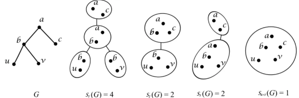
a 1 s G b v u c a b v u c b b a (G) = 4 s2 a b v u c b b (G) = 2 s3 a b v u c a (G) = 2 b v u c a k>3 s (G) = 1
Figure 2.1: Given a tree G with five vertices, for any k ≥ 1, a minimum size tree de-composition of width at most k is shown. So we see that s1(G) = 4, s2(G) = s3(G) = 2,
sk>3(G) = 1.
Related Work. In [DKZ13], Dereniowski et al. consider the problem of size-constrained path-decompositions. Given any positive integer k and any graph G with pathwidth at most k. Let lk(G) denote the smallest size of a path-decomposition of G with width at most k.
For any fixed k ≥ 4, computing lk is NP-complete in the class of general graphs and it is
NP-complete, for any fixed k ≥ 5, in the class of connected graphs [DKZ13]. Moreover, computing lk can be solved in polynomial-time in the class of graphs with pathwidth at
most k for any k ≤ 3. Finally, the “dual" problem is also hard: for any fixed s ≥ 2, it is NP-complete in general graphs to compute the minimum width of a tree-decomposition with size at most s. Note that this result was proved in [DKZ13] in terms of path-decomposition but it is straightforward to extend it to tree-decomposition.
2.2
NP-hardness in the class of bounded treewidth graphs
In this section, we prove that:
Theorem 4. For any fixed integer k ≥ 4 (resp., k ≥ 5), the problem of computing sk is
NP-complete in the class of graphs (resp., of connected graphs) with treewidth at most k. Note that the corresponding decision problem is clearly in NP. Hence, we only need to prove it is NP-hard.
Our proof mainly follows the one of [DKZ13] for size-constrained path-decompositions. Hence, we recall here the two steps of the proof in [DKZ13]. First, it is proved that, if computing lk is NP-hard for any k ≥ 1 in general graphs, then the
com-putation of lk+1 is NP-hard in the class of connected graphs. Second, it is shown that
computing l4is NP-hard in general graphs with pathwidth 4. In particular, it implies that
step consists of a reduction from the 3-PARTITION problem [GJ79] to the one of comput-ing l4. Precisely, for any instanceI of 3-PARTITION, a graph GI is built such thatI is a
YES instance if and only if l4(GI) equals some defined value `I.
Our contribution consists first in showing that the first step of [DKZ13] directly extends to the case of tree-decompositions. That is, it directly implies that, if computing sk is
NP-hard for some k ≥ 4 in general graphs, then so is the computation of sk+1 in the class of
connected graphs. Our main contribution of this section is to show that, for the graphs GI built in the reduction proposed in [DKZ13], any tree-decomposition of GI with width at most 4 and minimum size is a path decomposition. Hence, in this class of graphs, l4= s4
and, for any instanceI of 3-PARTITION, I is a YES instance if and only if s4(GI) equals
some defined value `I. We describe the details as follows.
Lemma 1. If the problem of computing skfor an integer k≥ 1 is NP-complete in general
graphs, then the computation of sk+1is NP-complete in the class of connected graphs.
Proof. Let G be any graph. We construct an auxiliary connected graph G0from G by adding a vertex a adjacent to all vertices in V (G). Given two integers k, s ≥ 1, in the following, we prove that there is a tree decomposition of G with width at most k and size at most s if and only if there is a tree decomposition of G0with width at most k + 1 and size at most s.
First, assume that (T,X) is a tree decomposition of G with width at most k and size at most s. Add a in each bag ofX. Then we get a tree decomposition of G0with width at most k+ 1 and size at most s.
Now let (T0,X0) be a tree decomposition of G0with width at most k + 1 and size at most s. We are going to find a tree decomposition of G with width at most k and size at most s.
LetXabe the set of all bags inX0containing a. Let Tabe the subtree of T0induced by
the bags inXa. Every vertex v ∈ V (G) is contained in a bag inXabecause va ∈ E(G0). For
any edge uv ∈ E(G), there is a bag X ⊇ {a, u, v} inX0 since {a, u, v} induces a clique in G0. So X ∈Xa. Delete a in each bag ofXaand denoteX−as the obtained set of bags. So
(Ta,X−) is a tree decomposition of G with width at most k and size at most s.
Before doing the reduction from the 3-PARTITIONproblem to the problem of comput-ing s4, let us first recall its definition.
Definition 2. [3-PARTITION]
Instance: A multiset S of3m positive integers S = (w1, . . . , w3m) and an integer b.
Question: Is there a partition of the set {1, . . . , 3m} into m sets S1, . . . , Sm such that
∑i∈Sjwi= b for each j = 1, . . . , m?
This problem is NP-complete even if |Sj| = 3 for all j = 1, . . . , m [GJ79].
Given an instance of 3-PARTITION, in the following, we construct a disconnected graph G(S, b) as in [DKZ13].
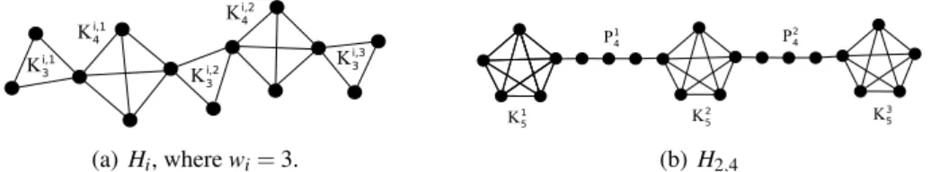
First, for each i ∈ {1, . . . , 3m}, we construct a connected graph Hi as follows. Take wi
copies of K3, denoted by K3i,q , q = 1, . . . , wi, and wi− 1 copies of K4, denoted by K4i,q ,
q= 1, . . . , wi− 1 (the copies are mutually disjoint). Then for each q = 1, . . . , wi− 1, we
identify two different vertices of K4i,q with a vertex of K3i,q and with a vertex of K3i,q+1, respectively. This is done in such a way that each vertex of each K3i,q is identified with
3 i,1 K 3 i,2 K 3 i,3 K 4 i,1 K 4 i,2 K (a) Hi, where wi= 3. 5 1 K 5 2 K 5 3 K 4 1 P 4 2 P (b) H2,4
Figure 2.2: Examples of gadgets in graph G(S, b).
at most one vertex from other cliques. Informally the cliques form a ’chain’ in which the cliques of size 3 and 4 alternate. See Figure 2.2(a) for an example of Hiwhere wi= 3.
Second, we construct a graph Hm,b as follows. Take m + 1 copies of K5, denoted by
K51, . . . , K5m+1, and m copies of the path graph Pb of length b (Pb has b edges and b + 1
vertices), denoted by Pb1, . . . , Pm
b. (Again, the copies are taken to be mutually disjoint.)
Now, for each j = 1, . . . , m, identify one of the endpoints of Pbj with a vertex of K5j, and identify the other endpoint with a vertex of K5j+1. Moreover, do this in a way that ensures that, for each j, no vertex of K5jis identified with the endpoints of two different paths. See Figure 2.2(b) for an example of H2,4. This implies that the computation of s4is NP-hard.
Let G(S, b) be the graph obtained by taking the disjoint union of the graphs H1, . . . , H3m
and the graph Hm,b. In the following, we prove that there is a tree decomposition of G(S, b)
of width 4 and size at most s = 1 − 2m + 2 ∑3mi=1wi if and only if there is a partition of the
set {1, . . . , 3m} into m sets S1, . . . , Sm such that ∑i∈Sjwi= b for each j = 1, . . . , m in the instance of 3-PARTITION.
In Lemma 2.2 of [DKZ13], they constructed a path decomposition of G(S, b) of width 4 and length 1 − 2m + 2 ∑3mi=1wi if there is a partition of the set {1, . . . , 3m} into m sets
S1, . . . , Sm such that ∑i∈Sjwi = b for each j = 1, . . . , m in the instance of 3-PARTITION. Obviously, this path decomposition is also a tree decomposition of G(S, b) of width 4 and size s. So we have the following lemma.
Lemma 2. Given a multiset S of 3m positive integers S = (w1, . . . , w3m) and an integer b,
if there is a partition of the set{1, . . . , 3m} into m sets S1, . . . , Smsuch that ∑i∈Sjwi= b for each j= 1, . . . , m, then G(S, b) has a tree decomposition of width at most 4 and size at most s= 1 − 2m + 2 ∑3mi=1wi.
Now we prove the other direction.
Lemma 3. If G(S, b) has a tree decomposition (T,X) of width at most 4 and size at most s= 1 − 2m + 2 ∑3mi=1wi, then there is a partition of the set{1, . . . , 3m} into m sets S1, . . . , Sm
such that ∑i∈Sjwi= b for each j = 1, . . . , m.
Proof. Lemma 2.6 in [DKZ13] proved that if G(S, b) has a path decomposition (T,X) of width at most 4 and length at most 1 − 2m + 2 ∑3mi=1wi, then there is a partition of the set
{1, . . . , 3m} into m sets S1, . . . , Sm such that ∑i∈Sjwi = b for each j = 1, . . . , m. So it is enough to prove that any tree decomposition (T, X ) of G(S, b) of width at most 4 and size at most s = 1 − 2m + 2 ∑3mi=1wiis a path decomposition of G(S, b).
As proved in Lemma 2.3 of [DKZ13], each bag in (T, X ) contains exactly one of the cliques K3i,q, K4i,q, K5j. Indeed, each of these cliques has size at least 3. Moreover, any two
of them share at most one vertex, and no two cliques of size 3 (K3i,q) share a vertex. So each bag of (T,X) contains at most one of the cliques Ki,q
3 , K
i,q
4 , K
j
5. However, for any clique,
there is a bag in (T,X) containing its vertices. Since s equals the number of the cliques K3i,q, K4i,q, K5j, each bag of (T,X) contains exactly one of them.
Moreover let us prove that any edge in K4i,q, K5j, Pbj (i.e. both the two endpoints of the edge) are contained in exactly one bag. Since each bag in (T, X ) contains exactly one of the cliques K3i,q, K4i,q, K5j, the two endpoints of any edge in the paths Pb1, . . . , Pbmare contained in a bag containing some K3i,q. (The bags containing a K4i,q(resp. K5j) cannot add another two vertices (one vertex) since (T,X) is a tree decomposition of width at most 4.) Every bag containing some K3i,qcontains at most one edge in the paths Pb1, . . . , Pbm, because the bag can add at most another two vertices and any K3i,q and Pbj are disjoint. There are mb edges in the paths Pb1, . . . , Pbmand there are mb bags containing some K3i,q, so every bag containing a K3i,qcontains exactly one edge in the paths Pb1, . . . , Pbm. So any edge in the paths Pb1, . . . , Pbm is contained in exactly one bag. Also each bag containing some K3i,q contains 5 vertices, so it does not contains any edge (i.e. both its two endpoints) in K4i,qor K5j. Therefore, any edge on K4i,q, K5jare contained in exactly one bag.
Now we prove that there are only two leaves in T and so T is a path. If a bag con-taining some K3i,q and an edge uv on some path Pbj is a leaf bag in T , then its neighbor bag also contains u, v because both u and v are incident to other edges in G(S, b). This is a contradiction with any edge (its two endpoints) on Pbj are contained only in one bag. So any bag containing some K3i,q is not a leaf bag in T . Similarly, we can prove that any bag containing any K4i,qor K5j for 1 < j < m + 1 is not a leaf bag in T . Thus there are only two bags containing K51and K5m+1are leaves in T .
Then we get the following corollary.
Corollary 1. It is NP-complete to compute s4in the class of graphs of treewidth at most 4.
Theorem 4 follows from Lemma 1 and Corollary 1.
2.3
Notations and preliminaries
In this section, we present the definitions and notations used throughout the chapter and some well known facts about tree-decompositions.
2.3.1 Notations
Given a graph G = (V, E), for any S ⊆ V , For an integer c ≥ 0, a graph G = (V, E) is c-connectedif |V | > c and no subset V0⊆ V with |V0| < c is a separator in G. A 2-connected componentof G is a maximal 2-connected subgraph.
Let (T,X) be any tree-decomposition of G. Abusing the notations, we will identify a node t ∈ V (T ) and its corresponding bag Xt ∈X. This means that, e.g., instead of saying
t∈ V (T ) is adjacent to t0∈ V (T ) in T , we can also say that Xt∈X is adjacent to Xt0∈X in T. A bag B ∈X is called a leaf-bag if B has degree one in T. Let k ≥ 1 and G be a graph with tw(G) ≤ k. A subset B ⊆ V (G) is a k-potential-leaf if there is a tree-decomposition (T,X)