HAL Id: hal-01926379
https://hal.archives-ouvertes.fr/hal-01926379
Submitted on 19 Nov 2018
HAL is a multi-disciplinary open access
archive for the deposit and dissemination of
sci-entific research documents, whether they are
pub-lished or not. The documents may come from
teaching and research institutions in France or
abroad, or from public or private research centers.
L’archive ouverte pluridisciplinaire HAL, est
destinée au dépôt et à la diffusion de documents
scientifiques de niveau recherche, publiés ou non,
émanant des établissements d’enseignement et de
recherche français ou étrangers, des laboratoires
publics ou privés.
Distributed under a Creative Commons Attribution| 4.0 International License
Bridging the Semantic Web and NoSQL Worlds:
Generic SPARQL Query Translation and Application to
MongoDB
Franck Michel, Catherine Faron Zucker, Johan Montagnat
To cite this version:
Franck Michel, Catherine Faron Zucker, Johan Montagnat. Bridging the Semantic Web and NoSQL
Worlds: Generic SPARQL Query Translation and Application to MongoDB. Transactions on
Large-Scale Data- and Knowledge-Centered Systems XL, 11360, Springer, pp.125-165, 2019, LNCS, ISBN:
978-3-662-58664-8. �hal-01926379�
Generic SPARQL Query Translation and
Application to MongoDB
Franck Michel[0000−0001−9064−0463], Catherine
Faron-Zucker[0000−0001−5959−5561], and Johan Montagnat
Universit´e Cˆote d’Azur, Inria, CNRS, I3S, France
franck.michel@cnrs.fr, faron@i3s.unice.fr, johan.montagnat@cnrs.fr
Abstract. RDF-based data integration is often hampered by the lack of methods to translate data locked in heterogeneous silos into RDF representations. In this paper, we tackle the challenge of bridging the gap between the Semantic Web and NoSQL worlds, by fostering the de-velopment of SPARQL interfaces to heterogeneous databases. To avoid defining yet another SPARQL translation method for each and every database, we propose a two-phase method. Firstly, a SPARQL query is translated into a pivot abstract query. This phase achieves as much of the translation process as possible regardless of the database. We show how optimizations at this abstract level can save subsequent work at the level of a target database query language. Secondly, the abstract query is translated into the query language of a target database, taking into ac-count the specific database capabilities and constraints. We demonstrate the effectiveness of our method with the MongoDB NoSQL document store, such that arbitrary MongoDB documents can be aligned on exist-ing domain ontologies and accessed with SPARQL. Finally, we draw on a real-world use case to report experimental results with respect to the effectiveness and performance of our approach.
Keywords: Query rewriting, SPARQL, RDF, NoSQL, xR2RML, Linked Data
1
Introduction
The Resource Description Framework (RDF) [11] is increasingly adopted as the pivot format for integrating heterogeneous data sources. It offers a unified data model that allows building upon countless existing vocabularies and domain ontologies, while benefiting from Semantic Web’s reasoning capabilities. It also allows leveraging the growing, world-scale knowledge base referred to as the Web of Data. Today, increasing amounts of RDF data are published on the Web, no-tably following the Linked Data principles [2,19]. These data often originate from heterogeneous silos that are inaccessible to data integration systems and search engines. Hence, a first step to enabling RDF-based data integration consists in translating legacy data from heterogeneous formats into RDF representations.
During the last fifteen years, much work has investigated how to translate common databases and data formats into RDF. Relational databases were pri-marily targeted [36,34], along with a handful of data formats such as XML [3] and CSV [28]. Meanwhile, the database landscape has significantly diversified with the adoption of various non-relational models. Initially designed as the core system of Big Data Web applications, NoSQL databases have gained momentum and are now increasingly adopted as general-purpose, commonplace databases. Today, companies and institutions store massive amounts of data in NoSQL in-stances. So far however, these data often remain inaccessible to RDF-based data integration systems, and consequently invisible to the Web of Data. although unleashing their data could potentially spur new integration opportunities and push the Web of Data forward.
The Semantic Web and NoSQL worlds build upon very different paradigms that are challenging to bridge over: whereas the former handles highly connected graphs along with the rich expressiveness of SPARQL, the latter trades off query expressiveness for scalability and fast retrieval of denormalized data1. As a result
of these discrepancies, bridging the gap between those two worlds is a challenging endeavor.
Two strategies generally apply when it comes to access non-RDF data as RDF. In the graph materialization strategy, the transformation is applied ex-haustively to the database content, the resulting RDF graph is loaded into a triple store and accessed through a SPARQL query engine [18] or by derefer-encing URIs (as Linked Data). On the one hand, this strategy easily supports further processing or analysis, since the graph is made available at once. On the other hand, the materialized RDF graph may rapidly become outdated if the pace of database updates is high. Running the transformation process pe-riodically is a common workaround, but in the context of large data sets, the cost (in time, memory and CPU) of materializing and reloading the graph may become out of reach. To work out this issue, the query rewriting strategy aims to access heterogeneous databases as virtual RDF graphs. A query processor rewrites a SPARQL query into the query language of the target database. The target database query is evaluated at run-time such that only relevant data are fetched from the database and translated into RDF triples. This strategy better scales to big data sets and guarantees data freshness, but entails overheads that may penalize performances if complex analysis is needed.
In previous works we defined a generic mapping language, xR2RML [25], that enables the translation of a broad scope of data sources into RDF. The mapping instructs how to translate each data item from its original format into RDF triples, by adapting to the multiplicity of query languages and data models. We applied xR2RML to the MongoDB NoSQL document store2and we implemented the graph materialization strategy.
1We refer to key-value stores, document stores and column family stores but leave out
graph stores that generally come with a richer query expressiveness.
2
To cope with large and frequently updated data sets though, we wish to tackle the question of accessing such databases using the query rewriting strategy. Hence, to avoid defining yet another SPARQL translation method for each and every database, in this paper we investigate a general two-phase method. Firstly, given a set of xR2RML mappings, a SPARQL query is rewritten into a pivot abstract query. This phase achieves as much of the translation process as possible regardless of the database, and enforces early query optimizations. Secondly, the abstract query is translated into the target database query language, taking into account the specific database capabilities and constraints. We demonstrate the effectiveness of our method in the case of MongoDB, accessing arbitrary MongoDB documents with SPARQL. We show that we can always rewrite an abstract query into a union of MongoDB find queries that shall return all the documents required to answer the SPARQL query.
The rest of this article is organized as follows. After a review of SPARQL query rewriting approaches in section 2, we quickly remind the principles and main features of the xR2RML mapping language in section3. Then, in sections4
and5 we describe the two-phase method introduced above. In section6, we de-scribe a real-world use case and we report experimental results with respect to the effectiveness and performance of our approach. Finally, we discuss our solu-tion and envision some perspectives in secsolu-tion7, and we draw some conclusions in section8.
2
Related Works
2.1 Rewriting SPARQL to SQL and XQuery
Since the early 2000’s, various works have investigated methods to query legacy data sources with SPARQL. Relational databases (RDB) have caught much at-tention, either in the context of RDB-backed RDF stores [10,35,14] or using arbitrary relational schemas [5,38,29,31,32]. These methods harness the ability of SQL to support joins, unions, nested queries and various string manipulation functions. Typically, a conjunction of two SPARQL basic graph patterns (BGP) results in the inner join of their respective translations; their union results in a SQL UNION ALL clause; the SPARQL OPTIONAL clause results in a left outer join, and a SPARQL FILTER results in an encapsulating SQL SELECT WHERE clause.
Chebotko’s algorithm [10] focused on RDB-based triple stores. Priyatna et al. [29] extended it to support custom R2RML mappings (the W3C recommen-dation of an RDB-to-RDF mapping language [12]) while applying several query optimizations. Two limitations can be emphasized though: (i) R2RML map-pings must have constant predicates, i.e. the predicate term of the generated RDF triples cannot be built from database values; (ii) Triple patterns are consid-ered and translated independently of each other, even when they share SPARQL variables. The resulting SQL query embeds unnecessary complexity that is taken care of later on, in the SQL query optimization step. Unbehauen et al. [38] clear the first limitation by defining the concept of compatibility between the RDF
terms of a SPARQL triple pattern and R2RML mappings, which enables man-aging variable predicates. Furthermore, to address the second limitation, they pre-checking join constraints implied by shared variables in order to reduce the number of candidate mappings for each triple pattern. Yet again, two limitations can be noticed: (iii) References between R2RML mappings are not considered, hence joins implied by shared variables are dealt with but joins declared in the R2RML mapping graph are ignored. (iv) The rewriting process associates each part of a mapping to a set of columns, called column group, which enables filter, join and data type compatibility checks. This leverages SQL capabilities (CASE, CAST, string concatenation, etc.), making it hardly applicable out of the scope of SQL-based systems. In the three aforementioned approaches, the optimization is dependent on the target database language, and can hardly be generalized. In our attempt to rewrite SPARQL queries in the general case, such optimization are performed earlier, regardless of the target database capabilities.
In a somewhat different approach, Rodr´ıguez-Muro and Rezk [32] extend the ontop Ontology-Based Data Access (OBDA) system to support R2RML mappings. A SPARQL query and an R2RML mapping graph are translated into a Datalog program. This formal representation is used to combine and apply optimization techniques from logic programming and SQL querying. The optimized program is then translated into an executable SQL query.
Other approaches investigated the querying of XML databases in a rather similar philosophy. For instance, SPARQL2XQuery [4] relies on the ability of XQuery to support joins, nested queries and complex filtering. Typically, a SPARQL FILTER is translated into an encapsulating For-Let-Where XQuery clause.
Finally, it occurs that the rich expressiveness of SQL and XQuery makes it possible to translate a SPARQL 1.0 query into a single, possibly deeply nested, target query, whose semantics is provably strictly equivalent to that of the SPARQL query. Commonly, query optimization issues are addressed at the level of the produced target query, or they may even be delegated to the target database optimization engine. Hence, the above reviewed methods are tailored to the expressiveness of the target query language, such that SQL or XQuery specificities are woven into the translation method itself, which undermines the ability to use such methods beyond their initial scope.
2.2 Rewriting SPARQL to NoSQL
To the best of our knowledge, little work has investigated how to perform RDF-based data integration over the NoSQL family of databases. An early work3
has tackled the translation of CouchDB4 documents into RDF, but did not
addressed SPARQL rewriting. MongoGraph5is an extension of the AllegroGraph triple store to query arbitrary MongoDB documents with SPARQL. But very
3https://github.com/agrueneberg/Sessel 4
http://couchdb.apache.org/
5
much like the Direct Mapping [1] defined in the context of RDBs, both works come up with an ad-hoc ontology (e.g. each JSON field name is turned into a predicate) and hardly supports the reuse of existing ontologies. Tomaszuk proposed to use a MongoDB database as an RDF triple store [37]. In this context, the author devised a translation of SPARQL queries into MongoDB queries, that is however closely tied to the specific database schema and thus is unfit for arbitrary documents.
More in line with our work, Botoeva et al. proposed a generalization of the OBDA principles [30] to MongoDB [8]. They describe a two-step rewriting pro-cess of SPARQL queries into a MongoDB aggregate pipeline. In section 7, we analyze in further details the relationship between their approach and ours. Interestingly, to the best of our knowledge, only one approach tackled the key-value store subset of NoSQL databases. Mugnier et al. [26] define the NO-RL rule language that can express lightweight ontologies to be applied to key-value stores. Leveraging the formal semantics of NO-RL, they propose an algorithm to reformulate a query under a NO-RL ontology, but SPARQL is not considered.
Finally, since NoSQL document stores are based on JSON, let us mention the JSON-LD syntax that is meant for the serialization of Linked Data in the JSON format. When applied to existing JSON documents, a JSON-LD profile can be considered as a lightweight method to interpret JSON data as RDF. Such a profile could be exploited by a SPARQL rewriting engine to enable the querying of document stores with SPARQL. This approach would be limited though, since JSON-LD is not meant to describe rich mappings from JSON to RDF, but simply to interpret JSON as RDF. It lacks the expressiveness and flexibility required to align JSON documents with domain ontologies that may model data in a rather different manner. Besides, we do not want to define a method specifically tailored to MongoDB; our point is to provide a generic rewriting method that can be applied to the concrete case of MongoDB as well as various other databases.
3
The xR2RML Mapping Language
The xR2RML mapping language [25] intends to foster the translation of legacy data sources into RDF. It can describe the mapping of an extensible scope of databases to RDF, independently of any query language or data model. It is backward compatible with R2RML and relies on RML [13] for the handling of various data formats. It can translate data with mixed embedded formats and generate RDF collections and containers.
An xR2RML mapping defines a logical source (propertyxrr:logicalSource)
as the result of executing a query against an input database (xrr:query and rr:tableName). An optional iterator (value of propertyrml:iterator) can be ap-plied to each query result, and a xrr:uniqueRef property can identify unique fields. Data from the logical source is mapped to RDF terms (literal, IRI, blank node) by term maps. There exists four types of term maps: a subject map gener-ates the subject of RDF triples, predicate and object maps produce the predicate
and object terms, and an optional graph map is used to name a target graph. Listing 1.1 depicts two mappings <#Mbox> and <#Knows>, each consisting of a subject map, a predicate map and an object map.
Term maps extract data from query results by evaluating xR2RML references whose syntax depends on the target database and is an implementation choice: typically, this may be a column name in case of a relational database, an XPath expression in case of an XML database, or a JSONPath6 expression in case of
NoSQL document stores like MongoDB or CouchDB. xR2RML references are used with property xrr:reference whose value is a single xR2RML reference, and property rr:templatewhose value is a template string which may contain several references. In Listing1.1, both subject maps use a template to build IRI terms by concatenating http://example.org/member/with the value of the "id"
JSON field. <# Mbox > xrr xrr xrr : l o g i c a l S o u r c el o g i c a l S o u r c el o g i c a l S o u r c e [ xrrxrrxrr :q u e r yq u e r yq u e r y " db . p e o p l e . f i n d ({ ’ emails ’:{ $ne : n u l l } } ) " ]; rr rr rr :s u b j e c t M a ps u b j e c t M a ps u b j e c t M a p [ rrrrrr :t e m p l a t et e m p l a t et e m p l a t e " h t t p :// e x a m p l e . org / m e m b e r /{ $ . id }" ]; rr rr rr : p r e d i c a t e O b j e c t M a pp r e d i c a t e O b j e c t M a pp r e d i c a t e O b j e c t M a p [ rr rrrr :p r e d i c a t ep r e d i c a t ep r e d i c a t e f o a f : m b o x ; rr
rrrr :o b j e c t M a po b j e c t M a po b j e c t M a p [ rrrrrr :t e m p l a t et e m p l a t et e m p l a t e " m a i l t o :{ $ . e m a i l s . * } " ; rrrrrr :t e r m T y p et e r m T y p et e r m T y p e rrrrrr :IRIIRIIRI ] ]. <# Knows > xrr xrr xrr : l o g i c a l S o u r c el o g i c a l S o u r c el o g i c a l S o u r c e [ xrr xrrxrr :q u e r yq u e r yq u e r y " db . p e o p l e . f i n d ({ ’ c o n t a c t s ’:{ $ s i z e : { $ g t e : 1 } } } ) " ]; rr rr rr :s u b j e c t M a ps u b j e c t M a ps u b j e c t M a p [ rrrrrr :t e m p l a t et e m p l a t et e m p l a t e " h t t p :// e x a m p l e . org / m e m b e r /{ $ . id }" ]; rr rr rr : p r e d i c a t e O b j e c t M a pp r e d i c a t e O b j e c t M a pp r e d i c a t e O b j e c t M a p [ rr rrrr :p r e d i c a t ep r e d i c a t ep r e d i c a t e f o a f : k n o w s ; rr rrrr :o b j e c t M a po b j e c t M a po b j e c t M a p [ rrrrrr : p a r e n t T r i p l e s M a pp a r e n t T r i p l e s M a pp a r e n t T r i p l e s M a p <# Mbox >; rrrrrr : j o i n C o n d i t i o nj o i n C o n d i t i o nj o i n C o n d i t i o n [ rrrrrr :c h i l dc h i l dc h i l d " $ . c o n t a c t s . * " ; rrrrrr :p a r e n tp a r e n tp a r e n t " $ . e m a i l s .*" ] ] ].
Listing 1.1. xR2RML example mapping graph
When the evaluation of an xR2RML reference produces several RDF terms, the xR2RML processor creates one triple for each term. Alternatively, therr:termType
property of a term map can be used to group the terms in an RDF collection while specifying a language tag or data type. Besides, the default iteration model can be modified using nested term maps, notably useful to parse nested collec-tions of values and generate appropriate triples.
xR2RML allows to model cross-references by means of referencing object maps that use values produced by the subject map of a parent mapping as the objects of triples produced by a child mapping. Properties rr:child and
rr:parentspecify the join condition between documents of both mappings. Running Example. To illustrate the description of our method, we define a running example that we shall use throughout this paper. Let us consider a MongoDB database with a collectionpeopledepicted in Listing1.2: each JSON
document provides the identifier, email addresses and contacts of a person; con-tacts are identified by their email addresses.
Let us now consider the xR2RML mapping graph in Listing1.1, consisting of two mappings<#Mbox>and<#Knows>. The logical source of mappings<#Mbox>,
6
{ "ididid ": 105632 , "f i r s t n a m ef i r s t n a m ef i r s t n a m e ":" J o h n " ,
"e m a i l se m a i l se m a i l s ": [" j o h n @ f o o . com " ," j o h n @ e x a m p l e . org "] , "c o n t a c t sc o n t a c t sc o n t a c t s ": [" c h r i s @ e x a m p l e . org " , " a l i c e @ f o o . com "] } { "ididid ": 327563 ,
"f i r s t n a m ef i r s t n a m ef i r s t n a m e ":" A l i c e " ,
"e m a i l se m a i l se m a i l s ": [" a l i c e @ f o o . com "] , "c o n t a c t sc o n t a c t sc o n t a c t s ": [" j o h n @ f o o . com "] }
Listing 1.2. MongoDB collection “people” containing two documents
respectively <#Knows>, is a MongoDB query that retrieves documents having a non-null emails field, respectively a contacts array field with at least one element. Both subject maps use a template to build IRI terms by concatenating
http://example.org/member/ with the value of JSON field id. Applied to the documents in Listing 1.2, the xR2RML mapping graph generates the following RDF triples: < h t t p :// e x a m p l e . org / m e m b e r / 1 0 5 6 3 2 > f o a f : m b o x < m a i l t o : j o h n @ f o o . com > , < m a i l t o : j o h n @ e x a m p l e . org >; f o a f : k n o w s < h t t p :// e x a m p l e . org / m e m b e r / 3 2 7 5 6 3 > . < h t t p :// e x a m p l e . org / m e m b e r / 3 2 7 5 6 3 > f o a f : m b o x < m a i l t o : a l i c e @ f o o . com >; f o a f : k n o w s < h t t p :// e x a m p l e . org / m e m b e r / 1 0 5 6 3 2 > .
4
From SPARQL to Abstract Queries
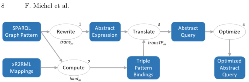
Section 2 emphasized that SPARQL rewriting methods for SQL or XQuery rely on prior knowledge about the target query language expressiveness. This makes possible the semantics-preserving translation of a SPARQL query into a single equivalent target query. In the general case however (beyond SQL and XQuery), the target query language may not support joins, unions, sub-queries and/or filtering. To tackle this challenge, our method first enacts the database-independent steps of the rewriting process. To generate the abstract query, we rely on and extend the R2RML-based SPARQL rewriting approaches reviewed in section2, while taking care of avoiding the limitations highlighted. More specif-ically, we focus on rewriting a SPARQL 1.0 graph pattern, whatever the query form (SELECT, ASK, DESCRIBE, etc.). The translation of a SPARQL graph pattern into an abstract query consists of four steps, sketched in Fig.1 and de-scribed in the next sub-sections. §4.1: A SPARQL 1.0 graph pattern is rewritten into an abstract expression exhibiting operators of the abstract query language. §4.2: We identify candidate xR2RML mappings likely to generate RDF triples that match each triple pattern. §4.3: Each triple pattern is translated into a sub-query according to the set of xR2RML mappings identified. A sub-sub-query consists of operators of the abstract query language and atomic abstract queries. §4.4: We enforce several optimizations on the resulting abstract query, e.g. self-joins or self-unions elimination.
Fig. 1. Translation of a SPARQL 1.0 graph pattern into an optimized abstract query
4.1 Translation of a SPARQL Graph Pattern
Our pivot abstract query language complies with the grammar depicted in Def.1. It derives from the syntax and semantics of SPARQL [27]: the language keeps the names of several SPARQL operators (UNION, LIMIT, FILTER) and prefers the SQL terms INNER JOIN ON and LEFT OUTER JOIN ON to refer to join operations more explicitly. A notable difference with SPARQL is that, in the tree representation of a query, the leaves of a SPARQL query are triple patterns. Conversely, the leaves of an abstract query are Atomic Abstract Queries (§4.3). The INNER JOIN and LEFT OUTER JOIN operators stem from the join constraints implied by shared variables. Somehow, the second INNER JOIN in Def.1, including the “AS child ” and “AS parent ” notations, is entailed by the join constraints expressed in xR2RML mappings using referencing object maps and propertiesrr:childandrr:parent. Notation v1,... vn, in the join operators,
stands for the set of SPARQL variables on which the join is to be performed. Notation <Ref> stands for any valid xR2RML data element reference, i.e. a col-umn name for a tabular data source, an XPath expression for an XML database, a JSONPath expression for a NoSQL document store such as MongoDB and CouchDB, etc.
Definition 1. Grammar of the Abstract Pivot Query Language
< A b s t r a c t Q u e r y > ::= < A t o m i c Q u e r y > | < Query > |
< Query > F I L T E RF I L T E RF I L T E R < S P A R Q L filter > | < Query > L I M I TL I M I TL I M I T < integer > < Query > ::= < A b s t r a c t Q u e r y > I N N E RI N N E RI N N E R J O I NJ O I NJ O I N < A b s t r a c t Q u e r y > ONONON { v1,... vn} | < A b s t r a c t Q u e r y > ASASAS c h i l d I N N E RI N N E RI N N E R J O I NJ O I NJ O I N < A b s t r a c t Q u e r y > ASASAS p a r e n t ON ONON c h i l d / < Ref > = p a r e n t / < Ref > | < A b s t r a c t Q u e r y > L E F TL E F TL E F T O U T E RO U T E RO U T E R J O I NJ O I NJ O I N < A b s t r a c t Q u e r y > ONONON { v1,... vn}| < A b s t r a c t Q u e r y > U N I O NU N I O NU N I O N < A b s t r a c t Q u e r y > < A t o m i c Q u e r y > ::= { From , Project , Where , L i m i t }
The first query transformation step is implemented by function transm
de-picted in Def.2. It rewrites a well-designed SPARQL graph pattern [27] into an abstract query while making no assumption with respect to the target database query capabilities. It extends the algorithms proposed in [10], [38] and [29].
Definition 2. Translation of a SPARQL query into an abstract query under xR2RML mappings (function transm).
Let m be an xR2RML mapping graph consisting of a set of xR2RML mappings. Let gp be a well-designed SPARQL graph pattern, f be a SPARQL filter and l an integer limit value representing the maximum number of results.
We denote by transm(gp, f, l) the translation, under m, of “gp FILTER f ” into an
abstract query that shall not return more than l results. We denote by transm(gp) the
result of transm(gp, true, ∞). Function transmis defined recursively as follows:
– if gp consists of a single triple pattern tp, transm(gp, f, l) = transTPm(tp,
spar-qlCond(tp, f ), l)
where transTPm translates a single triple pattern into an abstract query (§4.3)
and sparqlCond discriminates SPARQL filter conditions (§4.1). – if gp is (P LIMIT l’), transm(gp, f, l) = transm(gp, f, min(l, l’))
– if gp is (P FILTER f ’), transm(gp, f, l) = transm(P, f ∧ f ’, ∞) FILTER
spar-qlCond(P, f ∧ f ’) LIMIT l
– if gp is (P1 AND P2), transm(gp, f, l) = transm(P1, f, ∞) INNER JOIN
transm(P2, f, ∞) ON var(P1) ∩ var(P2) LIMIT l
– if gp is (P1 OPTIONAL P2), transm(gp, f, l) =
transm(P1, f, ∞) LEFT OUTER JOIN transm(P2, f, ∞) ON var(P1) ∩
var(P2) LIMIT l
– if gp is (P1 UNION P2), transm (gp, f, l) = transm (P1, f, l) UNION transm
(P2, f, l) LIMIT l
As a simplification, notations “FILTER true” and “LIMIT ∞” may be omitted.
Example. Let us give a first simple illustration. SPARQL query Q1 contains a
graph pattern gp1 that consists of two triple patterns, tp1 and tp2: Q1: S E L E C TS E L E C TS E L E C T ? x W H E R EW H E R EW H E R E {
? x f o a f : m b o x ? m b o x . # tp1
? x f o a f : k n o w s ? y . } # tp2
The application of function transm to the graph pattern gp1 is as follows: t r a n sm( gp1)
= t r a n sm( gp1, true , ∞)
= t r a n s T Pm( tp1, true , ∞) I N N E RI N N E RI N N E R J O I NJ O I NJ O I N
t r a n s T Pm( tp2, true , ∞) ONONON { var ( tp1) ∩ var ( tp2)}
L I M I T ∞
= t r a n s T Pm( tp1) I N N E RI N N E RI N N E R J O I NJ O I NJ O I N t r a n s T Pm( tp2) ONONON {? x }
Dealing with SPARQL filters. SPARQL rewriting methods reviewed in sec-tion2generally adopt a bottom-up approach where, typically, a SPARQL FIL-TER translates into an encapsulating query (e.g. a SELECT-WHERE clause in the case of SQL). Thus, filters in the outer query do not contribute to the selectivity of inner-queries that may return large intermediate results. This flaw is commonly worked out in a subsequent SQL query optimization step, or by assuming that the underlying database engine can take care of this optimization. In our context though, we cannot assume that the target query can be op-timized nor that the database query engine is capable of doing it. We therefore
consider SPARQL filters at the earliest stage: function transm pushes SPARQL
filters down into the translation of each inner query in order to return only necessary intermediate results.
Let us consider a SPARQL filter f as a conjunction of n conditions (n ≥ 1):
C1∧ ... Cn. Function sparqlCond, formally defined in [22], discriminates between
these conditions with regards to two criteria:
(i) A condition Ciis pushed into the translation of triple pattern tp if all variables
of Ci show up in tp, e.g. a condition involving variables ?x and ?y is pushed into
the translation of tp only if tp involves at least ?x and ?y.
(ii) A condition Ci is part of the abstract FILTER operator if at least one
variable of Ciis shared by several triple patterns, e.g. if Cicontains variable ?x,
and variable ?x also shows up in two different triple patterns, then Ci is in the
condition of the abstract FILTER operator.
Note that both criteria are not exclusive: a condition may simultaneously show up in the translation of a triple pattern and in the FILTER abstract operator. Example. SPARQL query Q2, depicted in Listing1.3, contains the graph
pat-tern gp2 that consists of three triple patterns tp1, tp2and tp3, and a filter
con-sisting of the conjunction of two conditions c1and c2: S E L E C TS E L E C TS E L E C T ? x W H E R EW H E R EW H E R E { ? x f o a f : m b o x ? m b o x . # tp1 ? y f o a f : m b o x < m a i l t o : j o h n @ f o o . com >. # tp2 ? x f o a f : k n o w s ? y . # tp3 F I L T E R F I L T E RF I L T E R { c o n t a i n s ( str (? m b o x ) , " foo . com ") # c1 && ? x != ? y } } # c2
Listing 1.3. SPARQL query Q2
Let us compute function sparqlCond for each triple pattern:
- tp1has two variables, ?x and ?mbox. No condition involves both variables, but
c1involves ?mbox and has no other variable, thereby c1matches criterion (i) for
tp1. Condition c2involves ?x but it also involves ?y that is not in tp1. Hence, c2
does not match criterion (i) for tp1, andsparqlCond(tp1, c1 ∧ c2) = c1.
- tp2has one variable, ?y, and no condition involves only ?y. Hence, no condition
can be pushed into the translation of tp2, denoted
sparqlCond(tp2, c1 ∧ c2) = true.
- tp3 has two variables ?x and ?y, and only condition c2 involves them both.
Hence, only c2matches criterion (i) for tp3 andsparqlCond(tp3, c1 ∧ c2) = c2.
- Lastly, only condition c2 involves variables shared by several triples patterns:
?x and ?y. Thus, only c2 matches criterion (ii), which entails the generation of
the abstract filterFILTER(c2).
As a result, gp2is rewritten into the following abstract query: t r a n sm( gp2, c1 ∧ c2) = t r a n s T Pm( tp1, c1) I N N E R I N N E R I N N E R J O I NJ O I NJ O I N t r a n s T Pm( tp2, t r u e ) ONONON {} I N N E R I N N E R I N N E R J O I NJ O I NJ O I N t r a n s T Pm( tp3, c2) ONONON {? x ,? y } F I L T E R F I L T E R F I L T E R ( c2)
Dealing with the LIMIT solution modifier. Similar to the case of SPARQL filters, the common bottom-up approach of SQL rewriting methods consists in
rewriting a LIMIT into an encapsulating query. Thus, again, sub-queries may return unnecessary large intermediate results. Therefore, function transmpushes
the LIMIT value down into the translation of each triple pattern using the limit argument l, initialized to ∞. During the parsing of the graph pattern by function transm, the limit argument is updated according to the graph pattern
encoun-tered. Below, we elaborate on some of the situations tackled in Def.2:
- In a graph pattern P LIMIT l’, the smallest limit is kept, hence the min(l, l’) in transm(gp, f, min(l, l’)).
- In a graph pattern P FILTER f ’, we cannot know in advance how many results will be filtered out by the FILTER clause. Consequently, we have to run the query with no limit and apply the filter afterward. Hence the ∞ argument in
transm(P, f ∧ f ’, ∞) FILTER sparqlCond(...) LIMIT l.
- Similarly, in the case of an inner or left join, we cannot know in advance how many results will be returned. Consequently, the left and right queries alike are run with no limit first, the join is computed, and only then can we limit the number of results. Hence the ∞ argument in the expressions:
transm(P1,f,∞) ... INNER JOIN transm(P2,f,∞) ... LIMIT l.
Dealing with other solution modifiers. For the sake of simplicity, we do not describe in further details the management of SPARQL solution modifiers OFFSET, ORDER BY and DISTINCT. Let us simply mention that they are managed in the very same way as the SPARQL FILTER clause and LIMIT solution modifier, i.e. as additional parameters of the transm and transTPm
functions, and additional operators of the abstract query language.
4.2 Binding xR2RML Mappings to Triple Patterns
An important step in the rewriting process consists in figuring out which of the mappings are good candidates to answer the SPARQL query. More precisely, for each triple pattern tp of the SPARQL graph pattern, we must figure out which mappings can possibly generate triples that match tp. We call this the triple pattern binding7, defined in Def.3:
Definition 3. Triple Pattern Binding.
Let m be an xR2RML mapping graph consisting of a set of xR2RML mappings, and tp be a triple pattern. A mapping M ∈ m is bound to tp if it is likely to produce triples that match tp. A triple pattern binding is a pair (tp, MSet) where MSet is the set of mappings of m that are bound to tp.
Function bindm(Def.4) determines, for a graph pattern gp, the bindings of
each triple pattern of gp. It takes into account join constraints implied by shared
7We adapt the triple pattern binding proposed by Unbehauen et al. in [38], and we
assume that xR2RML mappings are normalized in the sense defined by [32], i.e. they contain exactly one predicate-object map with exactly one predicate map and one object map, and any rr:class property is replaced by an equivalent predicate-object map with a constant predicate rdf:type
variables and by cross-references defined in the mapping (xR2RML referencing-object map), and the SPARQL filter constraints whose unsatisfiability can be verified statically. This is achieved by means of two functions: compatible and reduce. These functions were introduced in [38] but important details were left untold. Especially, the authors did not formally define what the compatibility between a term map and a triple pattern term means, and they did not investi-gate the compatibility between a term map and a SPARQL filter. In this section we give a detailed insight into these functions. A formal definition is provided in [22].
Definition 4. Binding xR2RML mappings to triple patterns (bindm).
Let m be a set of xR2RML mappings, gp be a well-designed graph pattern, and f be a SPARQL filter. Let M.sub, M.pred and M.obj respectively denote the subject map, the predicate map and the object map of an xR2RML mapping M.
We denote by bindm(gp, f ) the set of triple pattern bindings of “gp FILTER f ”
under m, and we denote by bindm(gp) the result of bindm(gp, true).
Function bindm(gp, f ) is defined recursively as follows:
– if gp consists of a single triple pattern tp, bindm(gp, f ) is the pair (tp, MSet)
where MSet = {M | M ∈ m ∧ compatible(M.sub, tp.sub, f ) ∧ compati-ble(M.pred, tp.pred, f ) ∧ compatible(M.obj, tp.obj, f )}
where compatible verifies the compatibility between a term map, a triple pattern term and a SPARQL filter
– if gp is (P1 AND P2), bindm(gp, f ) = reduce(bindm(P1, f ), bindm(P2,
f )) ∪ reduce(bindm(P2, f ), bindm(P1, f ))
where reduce utilizes dependencies between graph patterns to reduce their bindings
– if gp is (P1 OPTIONAL P2), bindm(gp, f ) = bindm(P1, f ) ∪ reduce(bindm(P2,
f ), bindm(P1, f ))
– if gp is (P1 UNION P2), bindm(gp, f ) = bindm(P1, f ) ∪ bindm(P2, f )
– if gp is (P FILTER f ’), bindm(gp, f ) = bindm(P, f ∧ f ’)
Function compatible checks whether a term map is compatible with (i) a term of a triple pattern and (ii) a SPARQL filter, so as to rule out incompatible asso-ciations. When the triple pattern term is constant (literal, IRI or blank node), incompatibilities may occur when its type does not mach the term map type (e.g. when the triple pattern term is a literal whereas the term map produces IRIs). Incompatibilities may also occur for literals when language tags or data types do not match. When the triple pattern term is a variable, incompatibil-ities may arise from unsatisfiable SPARQL filters. These situations pertain to type constraints expressed using SPARQL functions isIRI, isLiteral or isBlank, as well as language and data type constraints expressed using functions lang, langMatches and datatype. For instance, if variable ?v is associated with a term map that produces literals, the SPARQL filter isIRI(?v) can never be satisfied, which ensures that the association is invalid. We provided a formal definition of function compatible in [23].
Function reduce uses the variables shared by two triple patterns to detect unsatisfiable join constraints, and accordingly to reduce the set of mappings bound to each triple pattern. For instance, let us consider two triple patterns tp1 and tp2 that have a shared variable ?v. Mapping M1 is bound to tp1 and
mapping M2 is bound to tp2. If the term map associated to ?v in M1 generates
literals whereas the term map associated to ?v in M2 generates IRIs, we say
that the term maps are incompatible. Consequently, function reduce rules out M1 from the bindings of tp1 and M2 from the bindings of tp2. In other words,
reduce(bindm(tp1), bindm(tp2)) returns the reduced bindings of tp1 such that
the term maps associated to ?v in the bindings of tp1 are compatible with the
term maps associated to ?v in the bindings of tp2.
Running Example. Let us consider query Q2 depicted in Listing1.3. We first
compute the triple pattern bindings for tp1, tp2 and tp3 independently. The
constant predicate of tp1and tp2matches the constant predicate map of mapping
<#Mbox>. The subject and object of tp1are both variables, and the constant object
of tp2 (<mailto:john@foo.com>) is compatible with the object map of<#Mbox>.
Hence,<#Mbox>is bound to both triple patterns:
bindm(tp1, c1 ∧ c2) = (tp1, {<#Mbox>})
bindm(tp2, c1 ∧ c2) = (tp2, {<#Mbox>})
Likewise, we can show that<#Knows> is bound to tp3:
bindm(tp3, c1 ∧ c2) = (tp3, {<#Knows>}).
Let us consider the join constraint implied by variable ?y:
? y f o a f : m b o x < m a i l t o : j o h n @ f o o . com >. # tp2
? x f o a f : k n o w s ? y . # tp3
?y is the subject in tp2 that is bound to <#Mbox>, ?y is thereby associated to
<#Mbox>’s subject map. ?y is also the object in tp3that is bound to<#Knows>, ?y
is thereby associated to <#Knows>’s object map. Therefore, the expression reduce(bindm(tp2, c1 ∧ c2), bindm(tp3, c1 ∧ c2))
checks whether the subject map of<#Mbox>is compatible with the object map of
<#Knows>. But since the object map of<#Knows>is a referencing object map whose parent is <#Mbox>, this amounts to check whether the subject map of <#Mbox>
is compatible with itself, which is obvious. Consequently, the join constraint implied by variable ?y does not rule out any binding.
Similarly, we can show that the join constraint implied by variable ?x, shared by tp1 and tp3, does not rule out any binding. Lastly, the set of triple pattern
bindings for the graph pattern of query Q2is as follows:
bindm(tp1 AND tp2 AND tp3, c1 ∧ c2) =
(tp1,{<#Mbox>}), (tp2,{<#Mbox>}), (tp3,{<#Knows>})
4.3 Translation of a SPARQL Triple Pattern
The last step of the rewriting towards the abstract query language consists in the translation of each triple pattern into an abstract query, under the set of xR2RML mappings bound to that triple pattern by function bindm. This is
achieved by function transTPm defined in Def. 5, that may have to deal with
various situations.
Definition 5. Translation of a SPARQL Triple Pattern into Atomic Abstract Queries (function transTPm).
Let m be an xR2RML mapping graph consisting of a set of xR2RML mappings, gp be a well-designed graph pattern, and tp a triple pattern of gp. Let l be the maximum number of query results, and f be a SPARQL filter expression. Let getBoundMm(gp, tp, f ) be the function that, given gp, tp and f, returns the set
of mappings of m that are bound to tp in bindm(gp, f ).
We denote by transTPm(tp, f, l) the translation, under getBoundMm(gp, tp,
f ), of tp into an abstract query whose results can be translated into at most l RDF triples matching “tp FILTER f ”. The resulting abstract query, denoted <ResultQuery> in the grammar below, is a union of per-mapping subqueries, where a subquery is either an Atomic Abstract Query or the inner join of two Atomic Abstract Queries.
As a simplification, arguments f and l may be omitted when their values are “true” and ∞ respectively.
< R e s u l t Q u e r y > ::= < S u b Q u e r y > (U N I O NU N I O NU N I O N < S u b Q u e r y >)* < S u b Q u e r y > ::= < A t o m i c Q u e r y > |
< A t o m i c Q u e r y > ASASAS c h i l d I N N E RI N N E RI N N E R J O I NJ O I NJ O I N < A t o m i c Q u e r y > ASASAS p a r e n t ONONON c h i l d / < Ref >= p a r e n t / < Ref >
Let us now give an insight into how transTPmdeals with these situations.
(1) The most simple situation is encountered when a simple triple pattern tp is bound with a single xR2RML mapping M . If M has a regular object map (not a referencing object map denoting a cross-reference), then tp translates into an atomic abstract query. We will define the concept of atomic abstract query further on in this section. At this point, let us just notice that it is an abstract query obtained by matching the terms of a triple pattern with their respective term maps in a mapping.
(2) If the mapping M denotes a cross-reference by means of a referencing object map, .i.e. it refers to another mapping for the generation of object terms, then the result of transTPm is the INNER JOIN of two atomic abstract queries,
denoted:
< A t o m i c Q u e r y 1 > ASASAS c h i l d I N N E RI N N E RI N N E R J O I NJ O I NJ O I N < A t o m i c Q u e r y 2 > ASASAS p a r e n t ONONON c h i l d / c h i l d R e f = p a r e n t / p a r e n t R e f
where childRef and parentRef denote the values of properties rr:child and rr:parentrespectively.
(3) We have seen, in the definition of bindm, that several mappings may be
bound to a single triple pattern tp, each one may produce a subset of the RDF triples that match tp. In such a situation, transTPm translates tp into a union
of per-mapping atomic abstract queries.
Interestingly enough, we notice that INNER JOINs may be implied either by shared SPARQL variables (Def.2) or cross-references denoted in the mappings (situation (2) described above). Similarly, UNIONs may arise either from the
SPARQL UNION operator (Def. 2) or the binding of several mappings to the same triple pattern (situation (3) described above).
Due to size constraints, we do not go through the full algorithm of transTPm
in this paper, however the interested reader is referred to [22] for a comprehensive description.
Atomic Abstract Query. An atomic abstract query consists of four parts, denoted by {From, Project, Where, Limit}. We now describe these components and the way they are computed by function transTPm.
- From. The From part provides the concrete query that the abstract query relies on. It contains the logical source of an xR2RML mapping, that con-sists of the xrr:query or rr:tableName properties, an optional iterator (prop-ertyrml:iterator) and the optionalxrr:uniqueRefproperty. With the example of query Q2 (Listing 1.3), the From part for tp1 simply consists of the logical
source of <#Mbox>:db.people.find({’emails’:{$ne: null}}).
- Project . Traditionally, the projection part of a database query restricts the set of attributes that must be returned in the query response. In relational alge-bra, this is denoted by the projection operator π: πa1,...an(R) denotes the tuple
obtained when the attributes of tuple R are restricted to the set {a1, ...an}.
Simi-larly, the Project part of an atomic abstract query is a set of xR2RML references. For each variable in the triple pattern, the xR2RML references in the term map matched with that variable are projected. In our running example, the subject and object of tp1 are ?x and ?mbox1. They are matched with the subject and
object maps of mapping <#Mbox>. Thus, the corresponding xR2RML references within these subject map and object map must be projected. Hence the Project part for tp1: {$.id AS ?x, $.emails.* AS ?mbox1}. Furthermore, the child and
parent joined references of a referencing object map must be projected in order to accommodate databases that do not support joins. In the relational database case, these projections would be useless since the database can compute the join internally. But the abstract query must accommodate any target database, hence the systematic projection of joined references.
- Where. The Where part is a set of conditions about xR2RML references. They are produced by matching each term of a triple pattern tp with its corresponding term map in mapping M : the subject of tp is matched with M ’s subject map, the predicate with M ’s predicate map and the object with M ’s object map. Ad-ditional conditions are entailed from the SPARQL filter f. In [22], we show that three types of condition may be created:
(i) a SPARQL variable in the triple pattern is turned into a not-null condition on the xR2RML reference corresponding to that variable in the term map, denoted by isNotNull(<xR2RML reference>);
(ii) A constant term in the triple pattern (IRI or literal) is turned into an equal-ity condition on the xR2RML reference corresponding to that term in the term map, denoted by equals(<xR2RML reference>, value);
(iii) A SPARQL filter condition about a SPARQL variable is turned into a filter condition, denoted by sparqlFilter(<xR2RML reference>, f ).
t r a n st r a n st r a n sm( gp2) = t r a n s T P t r a n s T Pt r a n s T Pm( tp1, c1) I N N E RI N N E RI N N E R J O I NJ O I NJ O I N t r a n s T P t r a n s T Pt r a n s T Pm( tp2, t r u e ) ONONON {} I N N E RI N N E RI N N E R J O I NJ O I NJ O I N t r a n s T P t r a n s T Pt r a n s T Pm( tp3, c2) ONONON {? x ,? y } F I L T E R F I L T E RF I L T E R (? x != ? y ) t r a n s T Pt r a n s T Pt r a n s T Pm( tp1, c1) = { F r o mF r o mF r o m : {" db . p e o p l e . f i n d ({ ’ emails ’: {$ne : n u l l }})"} , P r o j e c t P r o j e c t P r o j e c t : {$. id ASASAS ? x , $. e m a i l s .* ASASAS ? m b o x 1 } , W h e r e W h e r e W h e r e : { i s N o t N u l li s N o t N u l li s N o t N u l l ($. id ) , i s N o t N u l li s N o t N u l li s N o t N u l l ($. e m a i l s .*) , s p a r q l F i l t e r s p a r q l F i l t e r s p a r q l F i l t e r ( c o n t a i n s ( str (? m b o x 1 ) ," foo . com " ) ) } } t r a n s T Pt r a n s T Pt r a n s T Pm( tp2, t r u e ) = { F r o mF r o mF r o m : {" db . p e o p l e . f i n d ({ ’ emails ’: {$ne : n u l l }})"} , P r o j e c t P r o j e c t P r o j e c t : {$. id ASASAS ? y } , W h e r e W h e r e W h e r e : { i s N o t N u l li s N o t N u l li s N o t N u l l ($. id ) , e q u a l se q u a l se q u a l s ($. e m a i l s .* ," j o h n @ f o o . com " ) } } t r a n s T Pt r a n s T Pt r a n s T Pm( tp3, c2) = { F r o mF r o mF r o m : {" db . p e o p l e . f i n d ({ ’ c o n t a c t s ’:{$ s i z e : {$gte : 1 } } } ) " } , P r o j e c t P r o j e c t P r o j e c t : {$. id ASASAS ? x , $. c o n t a c t s .*} , W h e r e W h e r e W h e r e : { i s N o t N u l li s N o t N u l li s N o t N u l l ($. id ) , i s N o t N u l li s N o t N u l li s N o t N u l l ($. c o n t a c t s .*) , s p a r q l F i l t e r s p a r q l F i l t e r s p a r q l F i l t e r (? x != ? y )}} ASASAS c h i l dc h i l dc h i l d I N N E RI N N E RI N N E R J O I NJ O I NJ O I N { F r o mF r o mF r o m : {" db . p e o p l e . f i n d ({ ’ emails ’:{$ne : n u l l } } ) " } , P r o j e c t P r o j e c t P r o j e c t : {$. e m a i l s .* , $. id ASASAS ? y } , W h e r e W h e r e W h e r e : { i s N o t N u l li s N o t N u l li s N o t N u l l ($. e m a i l s .*) , i s N o t N u l li s N o t N u l li s N o t N u l l ($. id ) , s p a r q l F i l t e r s p a r q l F i l t e r s p a r q l F i l t e r (? x != ? y )}} ASASAS p a r e n tp a r e n tp a r e n t ONONON c h i l dc h i l dc h i l d /$. c o n t a c t s .* = p a r e n tp a r e n tp a r e n t /$. e m a i l s .*
Listing 1.4. Rewriting of the graph pattern gp2 of query Q2 (Listing 1.3) into an
abstract query
Running Example. In the case of query Q2(Listing1.3), triple pattern tp2 is
matched with mapping <#Mbox>. It has the variable ?y in the subject position, which entails an isNotNull condition. It also has a constant term in the object position, which entails an equals condition. Finally, the Where part for tp2
con-tains two conditions:isNotNull($.id)andequals($.emails.*, "john@foo.com"). When we put all the pieces together, we can rewrite the graph pattern gp2 of
SPARQL query Q2 into the abstract query depicted in Listing1.4.
4.4 Abstract Query Optimization
At this point, the method we have exposed translates a SPARQL graph pattern into an effective abstract query, i.e. that preserves the semantics of the SPARQL query. Yet, shortcomings such as unnecessary complexity or re-dundancy may lead to the generation of inefficient queries, and consequently yield poor performances. Although we may postpone the query optimization to the translation into a concrete query language, it is beneficial to figure out which optimizations can be done at the abstract query level first, and leave only database-specific optimizations to the subsequent stage.
SPARQL-to-SQL methods proposed various SQL query optimizations such as [39,32,14]. In this section, we review some of these techniques, referring to the
t r a n st r a n st r a n sm( tp1 AND tp2 AND tp3 , c1 ∧ c2 ) = { F r o mF r o mF r o m : {" db . p e o p l e . f i n d ({ ’ emails ’:{$ne : n u l l }})"} , P r o j e c t P r o j e c t P r o j e c t : {$. id ASASAS ? x , $. e m a i l s .* ASASAS ? m b o x 1 } , W h e r eW h e r eW h e r e : { i s N o t N u l li s N o t N u l li s N o t N u l l ($. id ) , i s N o t N u l li s N o t N u l li s N o t N u l l ($. e m a i l s .*) , s p a r q l F i l t e rs p a r q l F i l t e rs p a r q l F i l t e r ( c o n t a i n s ( str (? m b o x 1 ) ," foo . com " ) ) } } I N N E R I N N E RI N N E R J O I NJ O I NJ O I N { F r o mF r o mF r o m : {" db . p e o p l e . f i n d ({ ’ c o n t a c t s ’:{$ s i z e : {$gte : 1 } } } ) " } , P r o j e c t P r o j e c t P r o j e c t : {$. id ASASAS ? x , $. c o n t a c t s .*} , W h e r eW h e r eW h e r e : { i s N o t N u l li s N o t N u l li s N o t N u l l ($. id ) , i s N o t N u l li s N o t N u l li s N o t N u l l ($. c o n t a c t s .*) , s p a r q l F i l t e rs p a r q l F i l t e rs p a r q l F i l t e r (? x != ? y )}} ASASAS c h i l dc h i l dc h i l d I N N E R I N N E RI N N E R J O I NJ O I NJ O I N { F r o mF r o mF r o m : {" db . p e o p l e . f i n d ({ ’ emails ’:{$ne : n u l l } } ) " } , P r o j e c t P r o j e c t P r o j e c t : {$. e m a i l s .* , $. id ASASAS ? y } , W h e r eW h e r eW h e r e : { i s N o t N u l li s N o t N u l li s N o t N u l l ($. e m a i l s .*) , i s N o t N u l li s N o t N u l li s N o t N u l l ($. id ) , e q u a l s e q u a l se q u a l s ($. e m a i l s .* ," j o h n @ f o o . com ") , s p a r q l F i l t e rs p a r q l F i l t e rs p a r q l F i l t e r (? x != ? y )}} ASASAS p a r e n tp a r e n tp a r e n t ON ONON c h i l dc h i l dc h i l d /$. c o n t a c t s .* = p a r e n tp a r e n tp a r e n t /$. e m a i l s .* ) ON ONON {? x ,? y } F I L T E R F I L T E RF I L T E R (? x != ? y )
Listing 1.5. Optimization of transm(gp2) (Listing1.4) by self-join elimination
terminology defined in [39]. We show how these optimizations can be adapted to fit in the context of our abstract query language. In particular, we show that our translation method implements some of these optimizations by construction. In addition, we propose a new optimization, the Filter Propagation, that, to our knowledge, was not proposed in any SPARQL-to-SQL rewriting method.
Filter Optimization. In a naive approach, strings generated by R2RML templates are dealt with using an SQL comparison of the resulting strings rather than the database values used in the template. Typically, when the translation of an R2RML template relies on the SQL string concatenation, a SPARQL query can ben rewritten into something like this:
S E L E C T ... F R O M ... W H E R E
( ’ h t t p :// d o m a i n / ’ || T A B L E . ID ) = ’ h t t p :// d o m a i n /1 ’
Such a query returns the expected results but is likely to perform very poorly: due to the concatenation, the query evaluation engine cannot take advantage of existing database indexes. Conversely, a much more efficient query would be:
S E L E C T ( ’ h t t p :// d o m a i n / ’ || T A B L E . ID ) . . . F R O M ... W H E R E T A B L E . ID = 1
In our approach, equality conditions apply to xR2RML references rather than on the template-generated values, hence the Filter Optimization is enforced by construction.
Filter pushing. As mentioned earlier, the translation of a SPARQL filter into an encapsulating SELECT WHERE clause lowers the selectivity of inner queries, and the query evaluation process may have to deal with unnecessarily large intermediate results. In our approach, Filter pushing is enforced by con-struction by the sparqlCond function: relevant SPARQL conditions are pushed down, as much as possible, in the translation of individual triple patterns.
Self-Join Elimination. A self-join may occur when several mappings share the same logical source. This can lead to several triple patterns being translated
into atomic abstract queries with the same From part. The Self-Join Elimination consists in merging the criteria of several atomic queries into a single equivalent query. In Listing1.4, the atomic query in transTPm(tp2, true) and the second
atomic query in transTPm(tp3, c2) have the same From part and project the
same JSONPath expression as variable?y. Using joins commutativity, those two queries can be merged into a single one depicted in the third atomic abstract query in Listing1.58.
Self-Union Elimination. A UNION operator can be created either due to the SPARQL UNION operator or during the translation of a triple pattern to which several mappings are bound (in function transT Pm). Analogously to the
Self-Join Elimination, a union of several atomic abstract queries sharing the same logical source can be merged into a single query when they have the same From part.
Constant Projection. The Constant Projection optimization detects cases where the only projected variables in the SPARQL query are matched with constant values in the bound mappings. In the relational database context, it has been referred to as the Projection Pushing optimization [39]. Let us consider the example query below:
S E L E C T D I S T I N C T ? p W H E R E {? s ? p ? o }.
In a naive approach, all mappings are bound to the triple pattern ?s ?p ?o. Hence, the resulting abstract query is a union of the atomic queries derived from all the possible mappings. In other words, this query will materialize the whole database before it can provide an answer. Very frequently, xR2RML predicate maps are constant-valued: the predicate is not computed from a database value, on the contrary it is defined statically in the mapping. This is typically the case in our running example that has only constant predicate maps (values of property rr:predicate: foaf:knows and foaf:mbox (Listing 1.1). In such cases, given that the SPARQL query retrieves only DISTINCT values of the predicate variable ?p, no query needs to be run against the database at all: it is sufficient to collect the distinct constant values that variable ?p can be matched with. More generally, this optimization checks if the variables projected in the SPARQL query are matched with constant term maps. If this is verified, the SPARQL query is rewritten such that the values of the projected variables be provided as an inline solution sequence using the SPARQL 1.1 VALUES clause. Using the mapping graph of our running example, we would rewrite the query in this way:
S E L E C T D I S T I N C T ? p W H E R E
{ V A L U E S ? p ( f o a f : m b o x f o a f : k n o w s )}
Filter Propagation. We identified another type of optimization that was not implemented in the SPARQL-to-SQL context. This optimization applies to the inner join or left outer join of two atomic queries, and seeks to narrow down one of the joined queries by propagating filter conditions from the other query. In an inner join, if the two queries have shared variables, then equals and isNotNull
8
Note that for a self-join elimination to be safe, additional conditions must be met, that we do not detail here.
AND ( < exp1> , < exp2> , . . . ) → $andandand :[ < exp1> , < exp2> ,...] OR ( < exp1> , < exp2> , . . . ) → $ororor :[ < exp1> , < exp2> ,...] W H E R E ( < J a v a S c r i p t exp >) → $wherew h e r ew h e r e : ’ < J a v a S c r i p t exp > ’ E L E M M A T C H ( < exp1> , < exp2>...) → $elemMatche l e m M a t c he l e m M a t c h :{ < exp1> , < exp2>...} F I E L D ( p1) ... F I E L D ( pn) → " p1. ... . pn":
S L I C E ( < exp > , < number >) → < exp >:{$slices l i c es l i c e : < number >} C O N D ( e q u a l s ( v )) → $eqeqeq : v
C O N D ( i s N o t N u l l ) → $existse x i s t se x i s t s :truetruetrue , $nenene :n u l ln u l ln u l l E X I S T S ( < exp >) → < exp >:{$existse x i s t se x i s t s :t r u et r u et r u e } N O T _ E X I S T S ( < exp >) → < exp >:{$existse x i s t se x i s t s :f a l s ef a l s ef a l s e } C O M P A R E ( < exp > , < op > , <v >) → < exp >:{ < op >: < v >} N O T _ S U P P O R T E D → ∅
U N I O N ( < query1 > , < query2 > . . . ) S a m e s e m a n t i c s as OR , a l t h o u g h OR is p r o c e s s e d by the N o S Q L e n g i n e w h e r e a s U N I O N is p r o c e s s e d by the q u e r y p r o c e s s i n g e n g i n e
Listing 1.6. Abstract representation of a MongoDB query and translation to a concrete query string. <op> stands for one of the MongoDB comparison operators: $eq, $ne, $lt, $lte, $gt, $gte, $size and $regex.
conditions of one query on those shared variables can be propagated to the other query. In a left join, propagation can happen only from right to left query since null values must still be allowed in the right query.
5
Application to the MongoDB NoSQL Database
In the previous section, we have exhibited an abstract query model and a method to translate a SPARQL graph pattern into an optimized abstract query, relying on the xR2RML mapping of a target database to RDF. We now want to illus-trate the effort it takes to translate from the abstract query language towards a concrete query language with a somewhat different expressiveness.
To this end, we consider the MongoDB NoSQL database. Its JSON-based data model and its query language differ greatly from SQL-based systems for which many rewriting works have been proposed. Hence, we believe that it should provide an interesting illustration of our method. Besides, MongoDB has become a popular NoSQL actor in recent years. It is provided as a service by major cloud service providers and tends to become common within the scientific community, suggesting that it is increasingly adopted as a commonplace database.
In this section, we first glance at the MongoDB query language, and we describe an abstract representation of MongoDB queries (section 5.1). Then, we show that the translation from the abstract query language towards Mon-goDB is made challenging by the expressiveness discrepancy between the two lan-guages (section5.2) and we describe a complete method to achieve this. Finally, we summarize the whole SPARQL-to-MongoDB process orchestration, from the SPARQL graph pattern translation until the generation of the RDF triples that match this graph pattern (section5.3).
5.1 The MongoDB Query Language
MongoDB comes with a rich set of APIs to allow applications to query a database in an imperative way. In addition, the MongoDB interactive interface defines a JSON-based declarative query language consisting of two query methods. The find method retrieves documents matching a set of conditions and returns a cur-sor to the matching documents. Optional modifiers amend the query to impose limits and sort orders. Alternatively, the aggregate method allows for the defini-tion of processing pipelines: each document of a collecdefini-tion passes through each stage of a pipeline thereby creating a new collection. This allows for a richer expressiveness but comes with a higher resource consumption that entails less predictable performances. Thus, as a first approach, this work considers the find query method, hereafter called the MongoDB query language.
The MongoDB find query method takes two arguments formatted as JSON documents. The first argument describes conditions about the documents to search for. Query operators are denoted by a heading ’$’ character. The optional projection argument specifies the fields of the matching documents to return. For instance, the query below matches all documents with a field “emails” and returns only the “id” field of each matching document.
db . p e o p l e . f i n d ({" e m a i l s ": {$ e x i s t s : t r u e }} , {" id ": t r u e })
The MongoDB documentation provides a rich description of the find query that however lacks precision as to the formal semantics of some operators. At-tempts were made to clarify this semantics while underlining some limitations and ambiguities: Botoeva et al. [7] mainly focus on the aggregate query and ignore some of the operators we use in our translation, such as $where, $elemM atch, $regex and $size. On the other hand, Husson [20] describes the find query, yet some restrictions on the operator $where are not formalized.
Hence, in [22] we specified the grammar of the subset of the query lan-guage that we consider. We also defined an abstract representation of MongoDB queries, that allows for handy manipulation during the query construction and optimization phases. Listing1.6details the constructs of this representation and their equivalent concrete query string, when relevant. The NOT SUPPORTED clause helps keep track of any location, within the query, where a condition can-not translate into an equivalent MongoDB query element. It shall be used in the last rewriting and optimization phase.
Let us consider the following abstract representation of a MongoDB query (or “abstract MongoDB query” for short):
AND ( C O M P A R E ( F I E L D ( p ) F I E L D (0) , $eq , 10) , F I E L D ( q ) E L E M M A T C H ( C O N D ( e q u a l s (" val ")) )
It matches all documents where “p” is an array field whose first element (at index 0) is 10, and “q” is an array field in which at least one element has value “val”. Its concrete representation is:
$and : [ {" p .0": {$eq :10}} ,
Fig. 2. Translation of atomic abstract queries into concrete MongoDB queries
5.2 Translation of an Abstract Query into MongoDB queries
Section 4 elaborated on how a SPARQL graph pattern translates into an ab-stract query based on xR2RML mappings. Abab-stract operators INNER JOIN, LEFT OUTER JOIN and UNION relate queries. The lowest level of sub-queries consists of atomic abstract sub-queries of the form {From, Project, Where, Limit}, that stem from the translation of individual triple patterns. The From part contains the logical source of a mapping bound to the triple pattern to translate. The Project part lists the xR2RML data element references that are projected, i.e. that are part of the query result. In the context of MongoDB, these xR2RML data element references are JSONPath expressions. The Where part is calculated by matching triple pattern terms with relevant xR2RML term maps. This generates conditions on JSONPath expressions (isNotNull conditions for SPARQL variables or equals conditions for constant triple pattern terms) and sparqlFilter conditions that encapsulate SPARQL filters. Finally, the Limit part denotes an optional maximum number of results.
To achieve a translation from the abstract query language towards the Mon-goDB query language, we must figure out which components of an abstract query have an equivalent MongoDB rewriting, and, conversely, which compo-nents shall be computed by the query-processing engine. Below, we analyze the possible situations.
- Inner and left outer joins. MongoDB find queries do not support joins. Consequently, there does not exist any MongoDB query that would be equiva-lent to the INNER JOIN and LEFT OUTER JOIN operators. These operators need to be processed by the query-processing engine by joining the RDF triples generated for both sub-queries.
- UNION. The rewriting of the UNION operator depends on the graph patterns to which it applies. Let us consider the following SPARQL graph pattern, where tpn is any triple pattern: { tp1. tp2. } UNION { tp3. tp4. } Each member
of the union translates into an INNER JOIN. Since joins cannot be processed within MongoDB, the outer UNION operator cannot be processed within Mon-goDB either. The issue occurs likewise as soon as one of the members is either an INNER JOIN or LEFT OUTER JOIN. Under some circumstances, a UNION operator may be translated into the MongoDB $or operator. Yet, the Mon-goDB language definition imposes specific restrictions as to how operators can be nested. Consequently, in a first approach, we always shift the processing of the UNION abstract operator to the query-processing engine. Further works could attempt to characterize more specifically the situations where a UNION can be processed within MongoDB.
- FILTER and LIMIT. In section4, we showed that the FILTER and LIMIT SPARQL solution modifiers are pushed down into relevant atomic abstract queries (as sparqlFilter conditions of the Where part or as the Limit part of an atomic query, respectively). When FILTER and LIMIT SPARQL clauses cannot be pushed down in atomic queries, they end up as abstract operators with the same names, FILTER and LIMIT. The latter apply to abstract sub-queries made of UNION, INNER JOIN and/or LEFT OUTER JOIN operators. Hence, given that UNION and INNER/LEFT OUTER JOIN operators are not processed within MongoDB, the FILTER and LIMIT operators cannot be processed within MongoDB either.
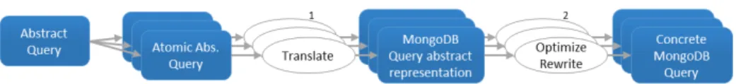
Ultimately, it occurs that only the atomic abstract queries can be processed within MongoDB, while other abstract operators shall be taken care of by the query-processing engine. More generally, the translation from the abstract query language towards MongoDB consists of two steps depicted in Fig. 2. In step 1 (detailed in section 5.2), the translation of each atomic abstract query towards MongoDB amounts to translate projections of JSONPath expressions (Project part) into MongoDB projection arguments, and conditions on JSONPath expres-sions (Where part) into equivalent abstract MongoDB queries. Several shortcom-ings may appear at this stage, such as unnecessary complexity or untranslatable conditions. Thus, in step 2 (detailed in section 5.2) each abstract MongoDB query is optimized and rewritten into valid, concrete MongoDB queries.
In the current status of this work, we do not consider the translation of SPARQL filters (conditions sparqlFilter ) for the sake of simplicity. SPARQL 1.0 filters come with a broad set of conditional expressions including logical com-parisons, literal manipulation expressions (string, numerical, boolean), XPath constructor functions, casting functions for additional data types of the RDF data model, and SPARQL built-in functions (lang, langmatches, datatype, bound, sameTerm, isIRI, isURI, isBlank, isLiteral, regex ). Handling these expressions within the translation towards MongoDB would yield a significant additional complexity without changing the translation principles though. Yet, an imple-mentation should handle them for the sake of performance and completeness. Translation of Projections and Conditions Two functions, named proj and trans, handle the translation of the Project and Where parts of an atomic abstract query respectively. Below, we illustrate their principles on an example. The interested reader shall find their formal definition in [22].
In Listing1.5, the third atomic abstract query is as follows (the sparqlFilter condition has been omitted):
{F r o mF r o mF r o m : {" db . p e o p l e . f i n d ({ ’ emails ’:{$ne : n u l l }})"} , P r o j e c t P r o j e c tP r o j e c t : {$. e m a i l s .* , $. id ASASAS ? y } , W h e r e W h e r eW h e r e : { i s N o t N u l li s N o t N u l li s N o t N u l l ($. e m a i l s .*) , i s N o t N u l li s N o t N u l li s N o t N u l l ($. id ) , e q u a l s e q u a l s e q u a l s ($. e m a i l s .* ," j o h n @ f o o . com ") }}
Function proj converts the JSONPath expressions of the From part into a list of paths to be projected. In the example, expressions$.emails.*and$.id trans-late into their MongoDB projection counterparts:"emails":trueand"id":true.
Fig. 3. Complete SPARQL-to-MongoDB Query Translation and Evaluation
Function trans translates a condition of the Where part into a MongoDB query element expressed using the abstract representation in Listing1.6. In the example, condition isNotNull($.emails.*) is translated into the following ab-stract representation:
FIELD(emails) ELEMMATCH(COND(isNotNull)).
Later on, this abstract representation will be translated into an equivalent con-crete query:
"emails": {$elemMatch: {$exists:true, $ne:null}}.
Similarly, conditionisNotNull($.id)will be translated into:"id": {$exists:true, $ne:null}, and conditionequals($.emails.*,"john@foo.com")will be translated
into: "emails": {$elemMatch: {$eq:’john@foo.com’}}.
These conditions are used to augment the query of the From part, initially provided by the mapping’s logical source. When we put all the pieces together, the atomic abstract query is translated into the concrete MongoDB query below, where all conditions are operands of an $and operator:
db . p e o p l e . f i n d ( # Q u e r y a r g u m e n t { $and : [ {" e m a i l s ": {$ne : n u l l }} , # f r o m the F r o m p a r t {" e m a i l s ": {$ e l e m M a t c h : {$ e x i s t s : true ,$ne : n u l l }}} , {" id ": {$ e x i s t s : true ,$ne : n u l l }} , {" e m a i l s ": {$ e l e m M a t c h : {$eq : ’ j o h n @ f o o . com ’ } } } ] } , # P r o j e c t i o n a r g u m e n t { " e m a i l s ": true , " id ": t r u e } )
Optimization and Rewriting into Concrete MongoDB Queries In the previous section, function trans produces abstract MongoDB queries that can be rewritten into concrete queries straightaway. Yet, this rewriting may be hindered by three potential issues: