HAL Id: hal-00966573
https://hal.archives-ouvertes.fr/hal-00966573
Submitted on 26 Mar 2014
HAL is a multi-disciplinary open access
archive for the deposit and dissemination of
sci-entific research documents, whether they are
pub-lished or not. The documents may come from
teaching and research institutions in France or
abroad, or from public or private research centers.
L’archive ouverte pluridisciplinaire HAL, est
destinée au dépôt et à la diffusion de documents
scientifiques de niveau recherche, publiés ou non,
émanant des établissements d’enseignement et de
recherche français ou étrangers, des laboratoires
publics ou privés.
Modeling Uncertainty when Estimating IT Projects
Costs
Michel Winter, Isabelle Mirbel, Pierre Crescenzo
To cite this version:
Michel Winter, Isabelle Mirbel, Pierre Crescenzo. Modeling Uncertainty when Estimating IT Projects
Costs. [Research Report] I3S. 2014. �hal-00966573�
LABORATOIRE
INFORMATIQUE, SIGNAUX ET SYSTÈMES DE SOPHIA ANTIPOLIS
UMR7271
Modeling Uncertainty when Estimating IT Projects Costs
Michel Winter, Isabelle Mirbel, Pierre Crescenzo
Équipe MODALIS - WIMMICSRapport de Recherche ISRN I3S/RR-2014-03-FR
Mars 2014
Laboratoire d'Informatique, Signaux et Systèmes de Sophia-Antipolis (I3S) - UMR7271 - UNS CNRS 2000, route des Lucioles - Les Algorithmes - bât. Euclide B 06900 Sophia Antipolis - France
Modeling Uncertainty when Estimating IT Projects Costs
Michel Winter 1, Isabelle Mirbel 2, Pierre Crescenzo3, Équipe MODALIS - WIMMICS
ISRN I3S/RR-2014-03-FR Mars 2014- 4 pages
Abstract: In the current economic context, optimizing projects' cost is an obligation for a company to remain competitive in
its market. Introducing statistical uncertainty in cost estimation is a good way to tackle the risk of going too far while minimizing the project budget: it allows the company to determine the best possible trade-off between estimated cost and acceptable risk. In this paper, we present new statistical estimators derived from the way IT companies estimate the projects' costs. In the current practice, the software to develop is progressively divided into smaller pieces until it becomes easy to estimate the associated development workload and the workloads of the usual additionnal activities (documentation, test, project management,...) are deduced from the development workload by applying ratios. Finally, the total cost is derived from the resulting workload by applying a daily rate. This way, the overall workload cannot be calculated nor estimated analytically. We thus propose to use Monte-Carlo simulations on PERT and dependency graphs to obtain the cost distribution of the project.
Key-words: IT Project ; Cost Estimation ; Monte-Carlo Method ; PERT
1 Univ. Nice Sophia Antipolis, 06900 Sophia Antipolis, France – [email protected]
2 Univ. Nice Sophia Antipolis, CNRS, I3S, UMR 7271, 06900 Sophia Antipolis, France – WIMMICS (Inria Sophia Antipolis / Laboratoire I3S) - [email protected]
Modeling Uncertainty when Estimating IT Projects Costs
Michel Winter
MIAGE,
Univ. Nice Sophia Antipolis, 1645 rte des Lucioles, 06900
Sophia Antipolis, France
[email protected]
Isabelle Mirbel
Univ. Nice Sophia Antipolis, CNRS, I3S, UMR 7271, 06900
Sophia Antipolis, France
[email protected]
Pierre Crescenzo
Univ. Nice Sophia Antipolis, CNRS, I3S, UMR 7271, 06900
Sophia Antipolis, France
[email protected]
ABSTRACT
In the current economic context, optimizing projects’ cost is an obligation for a company to remain competitive in its market.
Introducing statistical uncertainty in cost estimation is a good way to tackle the risk of going too far while minimiz-ing the project budget: it allows the company to determine the best possible trade-off between estimated cost and ac-ceptable risk.
In this paper, we present new statistical estimators derived from the way IT companies estimate the projects’ costs. In the current practice, the software to develop is progressively divided into smaller pieces until it becomes easy to esti-mate the associated development workload and the work-loads of the usual additionnal activities (documentation, test, project management,...) are deduced from the devel-opment workload by applying ratios. Finally, the total cost is derived from the resulting workload by applying a daily rate.
This way, the overall workload cannot be calculated nor es-timated analytically. We thus propose to use Monte-Carlo simulations on PERT and dependency graphs to obtain the cost distribution of the project.
1.
INTRODUCTION
When developping software, cost estimation can be reduced to effort estimation since the project cost is derived by ap-plying a daily rate.
The effort can be estimated in two ways: following an ap-proach relying on expert judgment or an apap-proach based on parametric models. Approaches based on expert judgment rely on a work breakdown structure; each task is sized based on an expert intuition and it is possible to model uncer-tainty by associating probabilistic distribution to each task estimate.
Concerning approaches relying on parametric models, many different types are available [2]. Even if model-based ef-fort estimation processes may rely very much on expert judgment-based input, propagating uncertainty within the
model becomes complicated.
In this paper we consider an hybrid approach, combining pure expert judgement for development task workload esti-mation and simple model-based estimators for other activi-ties. Uncertainty are introduced wherever expert inputs are required and propagated to the global project effort estima-tion.
The paper is organized as follows: in section 2, we intro-duce a running example to illustrate our approach. Section 3 is dedicated to related work. In Section 4, we discuss the model we propose to propagate uncertainty into cost mod-els. The way our model may be used on a concrete example is described in section 5. Finally, in section 6 we conclude the paper.
2.
RUNNING EXAMPLE
We explain our approach along with a running example which is presented in the following.
A simple software has to be developped. An expert analysed the software requirements and identified two development tasks named Dvt1 and Dvt2. He estimated the associated
development effort as follows:
• Dvt1 should costs 6± 1 man.days (md),
• Dvt2should also costs between 5 to 7md but it is more
likely to be closer to 5 rather than 7.
In addition to the development activity, the project manager establishes that for such kind of project the test activity, T st, represents 50% of the development effort Dvt1+ Dvt2, and
the reporting activities, Rpt, represents 1md every week, during the whole project duration. If we consider that the two development tasks can be performed simultaneously, the sequence diagram modeling the project is shown in figure 1. Since we have an uncertainty on Dvt1 and Dvt2 duration,
Dvt1
Dvt2 Tst
Rpt
End
Figure 1: Task sequencing graph
and since activities T st and Rpt depend on these develop-ment tasks, we need an approach to determine what is the best value to consider for the global effort and what is the resulting uncertainty.
3.
RELATED WORK
3.1
Tasks and distributions
In project management, the classic way to introduce uncer-tainty in project cost-or-duration computation consists in considering each estimation as a random variable associated to a beta distribution [4]. The beta distribution is defined as follows: f (x) = a + (b− a) xα−1(1−x)β−1 1 ∫ 0 uα−1(1−u)β−1du ∀x ∈ [a, b] 0 otherwise
with: a, b the minimum and maximum of the distri-bution,
α, β defining the support of the function shape parameters
Modeling task Dvt1 would lead to the following values: a =
5, b = 7, α = β = 2. The associated distribution is illus-trated in figure 2. Selecting α = β leads to a symmetrical
6 5 5.2 5.4 5.6 5.8 6.2 6.4 6.6 6.8 7 0 1 0.2 0.4 0.6 0.8 1.2 1.4 1.6
Figure 2: Beta distribution with a = 5, b = 7 and
α = β = 2
distribution centered around 6. It is also possible to model
Dvt2for witch the workload is likely to be closer to 5 by
set-ting β to 3 rather than 2, as shown in figure 3. Considering
6 5 5.2 5.4 5.6 5.8 6.2 6.4 6.6 6.8 7 0 1 0.2 0.4 0.6 0.8 1.2 1.4 1.6 1.8
Figure 3: Beta distribution with a = 5, b = 7, α = 2 and β = 3
a bigger project, each task i of the project can be modeled in the same way as a random variable Xidescribed by a beta
distribution with parameters ai, bi, αi and βi. The
work-load of the whole project is defined as the sum of all these random variables. The workload can then be determined in two ways:
• using the Central Limit Theorem or • applying Monte-Carlo simulations.
3.2
The Central Limit Theorem
The Central Limit Theorem (CLT) [11] states that the arith-metic mean of a sufficiently large number of iterates of inde-pendent random variables, each with a well-defined expected value and well-defined variance, will be approximately nor-mally distributed.
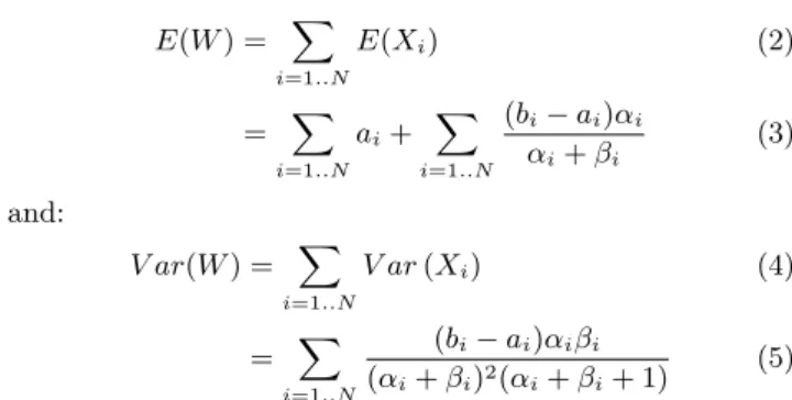
If we consider the random variable W associated to the project workload, defined as the sum of Xi random
vari-ables, we have:
W = ∑ i=1..N
Xi (1)
The CLT then states that W converges to a normal distribu-tion whose mean E(W ) and variance V ar(W ) are approxi-mated to: E(W ) = ∑ i=1..N E(Xi) (2) = ∑ i=1..N ai+ ∑ i=1..N (bi− ai)αi αi+ βi (3) and: V ar(W ) = ∑ i=1..N V ar (Xi) (4) = ∑ i=1..N (bi− ai)αiβi (αi+ βi)2(αi+ βi+ 1) (5)
CLT is an efficient tool to manage uncertainty within the workload estimation as it is defined in (1), but it requires strict conditions [9]:
• the final random variable is a sum of initial ones, • initial random variables must be identically distributed,
with finite mean and variance,
• initial random variables are independent,
• the sum of random variables tends to be normally
dis-tributed as the number of these variables increases. In practice, the approximation is considered as accept-able for a sum of 30 random variaccept-ables, even 50 if the distribution of random variables is asymmetric.
In the context described earlier, the second condition is not strictly fulfilled since different values for α and β lead to different distributions. An improvement to the CLT, named Lindberg’s condition, states that the convergence to a nor-mal distribution is also guaranteed if the second condition is omitted [8]. However, the first and third conditions are not fulfilled when considering our running example. Test and reporting activities are not terms that just have to be summed with development tasks and they are clearly corre-lated to the other tasks. CLT cannot be used.
3.3
Monte-Carlo experiments
The Monte-Carlo method is an alternative method allow-ing to compute complex combination of random variables. It relies on repeated random (statistical) sampling of ele-mentary random variables. Simulations are run many times over in order to calculate the resulting probability heuristi-cally. The algorithm is simple; the only complexity consists in generating samples according to associated distributions. It generally involves transforming a uniform random number in some way. Two methods are used [3]:
• the inversion method, that consists in integrating up to
an area greater than or equal to the random number;
• the acceptance-rejection method, involves choosing x
and y values according to a uniform distribution (the standard random function) and testing whether the distribution function of x is greater than the y value. If it is, the x value is accepted. Otherwise, the x value is rejected and the algorithm tries again.
This approach is a way to compute a numerical approxima-tion which error can be lowered by increasing the number of generated samples: if we denote R the number of generated sampling sets, the error is reduced by a factor of1/√R[7].
Since no condition is required unlike in the CLT approach, Monte-Carlo is clearly an approach that we can use to prop-agate uncertainty from expert inputs to the global effort. In order to achieve this, we are now going to elaborate the analytical model of the effort in accordance with the way it is expressed within the running example.
4.
A MODEL COMBINING
HETEROGENE-OUS TASK ESTIMATORS
As explained previously, development tasks are modeled us-ing beta distributions: the developer estimates what is the minimum and maximum time he would need to implement the associated feature (parameters a and b). Then he tunes the shape parameters α and β in order to reflect his feeling: will it be more likely close to the maximum b or to the min-imum a.
Let’s note Xithe associated random variables with Xi∈ Tβ,
where Tβ corresponds to the set of tasks that are modeled
using beta distributions.
When the effort associated to an activity is deduced by ap-plying a ratio to a set of other tasks workloads, the corre-sponding random variable is modeled as follows:
Xj= f (aj, bj, αj, βj)
∑
Xl∈T
δj,lXl (6)
where:
δj,l is a boolean value that defines the set of random
variables that are summed. δ4,8 = 1 means that
X8 is used in the calculation of X4.
T is the set containing all the tasks of the project.
Again, function f () represents the beta distribution; it al-lows to model the fact that the ratio may also be uncertain. Considering our running example, let’s name X1,X2 and X3
the random variables associated to tasks Dvt1, Dvt2 and
T st respectively. We can write:
X3= f (0.4, 0.6, 2, 2) (X1+ X2) (7)
= f (0.4, 0.6, 2, 2) ∑
Xl∈Tβ
δ3,lXl (8)
with δ3,1 = 1 and δ3,2 = 1. We also decided to add an
uncertainty to the ratio of 50%; so we replace it by a beta distribution taking its values between 0.4 and 0.5.
Finally, for task Rpt we need to introduce another type of estimator: a ratio is applied to the duration of a set of tasks. It requires that the scheduling of the different tasks has al-ready been elaborated. This schedule is defined as a directed
graph Gsched= (T, E) where T is the set of node; each node
represents a task of the project and E is a set of edges, i.e. pairs of T. The workload of each task is associated to each node. Finding the duration of a set of activities then con-sists in computing the longest path between the related start and ending nodes. Let’s note Dur(Gsched, s, e) the function
that computes the duration between the two nodes s and e within the graph Gsched, we have:
Xk= f (ak, bk, αk, βk)Dur (Gsched, sk, ek) (9)
In our example, graph Gsched is illustrated in figure 1. If
we note X4 the random variable associated to task Rpt, we
would write:
X4= f (0.15, 0.25, 2, 2)Dur (Gsched, Start, End) (10)
Again, we added an uncertainty to the ratio of 20%; these 20% represent the effort of 1md per week estimated in our running example.
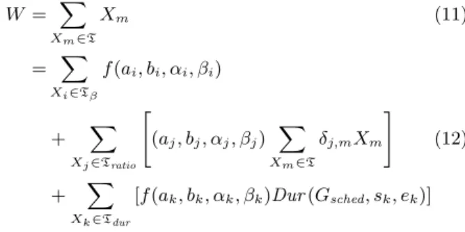
Our major contribution consists in the resulting global work-load W that is synthesized below:
W = ∑ Xm∈T Xm (11) = ∑ Xi∈Tβ f (ai, bi, αi, βi) + ∑ Xj∈Tratio [ (aj, bj, αj, βj) ∑ Xm∈T δj,mXm ] (12) + ∑ Xk∈Tdur [f (ak, bk, αk, βk)Dur (Gsched, sk, ek)]
Where Tratioand Tdurare the sets of random variables that
are calculated according to model (6) and (9) respectively.
5.
APPLYING MONTE-CARLO
SIMULATIONS
The random variables are clearly no more independent and the project workload is now more complex than a sum a initial random variables. As a result, it is not possible to calculate the project workload using the CLT. The Monte-Carlo method has to be used. However, the project cost as expressed in (12) raises two difficulties described hereafter.
5.1
Tasks dependency
Random variables from Tratioand Tdurdefine a dependency
graph Gdep= (T, E2), where the arcs within E2 are defined
by the adjacency matrix ∆, gathering δi,j as defined in (6).
The associated dependency graph is illustrated in figure 4.
Tst Dvt1
Dvt2
Rpt
To be able to compute W , it is necessary to derive an eval-uation order that respects the given dependencies. Cycles within Gdepwould lead to a situation in which no valid
eval-uation order exists, because none of the objects in the cycle may be evaluated first.
If it does not have any circular dependencies, the graph is a directed acyclic graph, and an evaluation order may be found by topological sorting. There are several algo-rithms that performs topological ordering; we used the one described in [6]. Considering our running example, the or-dering S ={X1, X2, X3, X4} is valid.
5.2
Tasks duration
For random variables from Tdur, we need to compute the
du-ration of a group of tasks. In graph theory, it consists in com-puting the longest path between two nodes wihtin Gsched.
Several algorithms answer this need but they all require edge-weighted graphs while we defined a vertex-weighted graph.
Therefore, Gschedhas to be converted into its edge-weighted
dual G′sched. In the dual graph, the edges represent the
ac-tivities, and the vertices represent the start or the finish of an activitiy. For this reason, the dual graph is also called an event-node graph.
The easiest way to tranform Gsched into G′sched is to replace
each node v in the original graph with two nodes, vin and vout, connected by a single edge with weight equal to the
original vertex weight. Then the original edges (u, v) are replaced with edges from uoutto vinof zero weight. Finally,
when an original node v has only one predecessor, vinis
re-moved. Considering our example, the resulting dual graph is shown in figure 5. End Dvt2-Out Dvt1-Out TstOut TstIn RptOut X1 X2 X4 X3
Ø
Ø
Ø
Ø
Figure 5: Scheduling dual graph
Since it is a directed acyclic graph, a longest path in the graph G′schedcorresponds to a shortest path in a graph−G′sched
derived from G′schedby changing every workload to its
nega-tion [10]. Longest paths in G′sched can be found in linear
time by applying a linear time algorithm for shortest paths in−G′sched such as [1, 5].
5.3
Running example
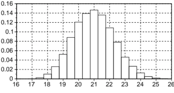
A Monte-Carlo simulation of 10000 turns has been performed on our running example; the repartition of the effort is given in figure 6. Using this distribution, we can easily tackle the uncertainty of our project. Depending on the way we want to manage the associated risk, two kind of questions can help the project manager in his decision making:
• What is the likehood that the project duration is for
instance less than 19 m.d? In our example, the answer is 4% 20 16 17 18 19 21 22 23 24 25 26 0 0.1 0.02 0.04 0.06 0.08 0.12 0.14 0.16
Figure 6: Distribution of the effort
• What is the maximal workload of the project, with a
likehood of 90%? The answer is 23 m.d
6.
CONCLUSION
In this paper we proposed new statistical estimators for ex-pert judgement-based effort estimation processes.
Because the global workload is a complex combination of random variables, it is not possible to calculate an analyt-ical expression of its distribution. The propagation of un-certainty within the global workload model thus requires a numerical approach such as the Monte-Carlo simulation. Even if the mean of the global workload could be easily de-termined without the help of Monte-Carlo simulation, our approach also provides an approximation of the workload distribution. This distribution allows the project manager to estimate more accurately the project cost and to better decide the maximum risk he can afford.
7.
REFERENCES
[1] R. Bellman. On a routing problem. Quarterly of
Applied Mathematics, 16:87–90, 1958.
[2] L. C. Briand and I. Wieczorek. Resource estimation in software engineering. In J. J. Marcinak, Encyclopedia
of software engineering, pages 1160–1196, 2002.
[3] L. Devroye. Non-Uniform Random Variate
Generation. Springer-Verlag, New York, 1986.
[4] P. M. Institute. A Guide to the Project Management
Body of Knowledge: PMBOK Guide. Newtown
Square, Pennsylvania, 2013.
[5] L. R. F. Jr. Network Flow Theory. RAND Corporation, 1956.
[6] A. B. Kahn. Topological sorting of large networks.
Communications of the ACM, 11(5):558–562, 1962.
[7] E. Koehler, E. Brown, and S. J.-P. A. Haneuse. On the assessment of monte carlo error in simulation-based statistical analyses. Am Stat, 63(2):155–162, 2009. [8] J. W. Lindeberg. Eine neue herleitung des
exponentialgesetzes in der
wahrscheinlichkeitsrechnung. Mathematische
Zeitschrift, 1(15):211–225, 1922.
[9] J. Rice. Mathematical Statistics and Data Analysis
(Second ed.). Duxbury Press, 1995.
[10] R. Sedgewick and K. D. Wayne. Algorithms (4th ed.). Addison-Wesley Professional, 2011.
[11] G. W. Snedecor and W. G. Cochran. Statistical
Methods, Eighth Edition. Iowa State University Press,