HAL Id: hal-02954424
https://hal.archives-ouvertes.fr/hal-02954424
Submitted on 28 Oct 2020
HAL is a multi-disciplinary open access
archive for the deposit and dissemination of
sci-entific research documents, whether they are
pub-lished or not. The documents may come from
teaching and research institutions in France or
abroad, or from public or private research centers.
L’archive ouverte pluridisciplinaire HAL, est
destinée au dépôt et à la diffusion de documents
scientifiques de niveau recherche, publiés ou non,
émanant des établissements d’enseignement et de
recherche français ou étrangers, des laboratoires
publics ou privés.
Andrew Schuh, Andrew Jacobson, Sourish Basu, Brad Weir, David Baker,
Kevin Bowman, Frederic Chevallier, Sean Crowell, Kenneth Davis, Feng Deng,
et al.
To cite this version:
Andrew Schuh, Andrew Jacobson, Sourish Basu, Brad Weir, David Baker, et al.. Quantifying the
Impact of Atmospheric Transport Uncertainty on CO 2 Surface Flux Estimates. Global
Biogeo-chemical Cycles, American Geophysical Union, 2019, 33 (4), pp.484-500. �10.1029/2018GB006086�.
�hal-02954424�
Andrew E. Schuh1 , Andrew R. Jacobson2, Sourish Basu2, Brad Weir3 , David Baker1,
Kevin Bowman4 , Frédéric Chevallier5 , Sean Crowell6 , Kenneth J. Davis7 ,
Feng Deng8 , Scott Denning9, Liang Feng10,11, Dylan Jones8 , Junjie Liu4 ,
and Paul I. Palmer10,11
1Cooperative Institute for Research in the Atmosphere, Colorado State University, Fort Collins, CO, USA,2University of Colorado Boulder and NOAA Earth System Research Laboratory, Boulder, CO, USA,3Global Modeling and
Assimilation Office, NASA Goddard Space Flight Center, Greenbelt, MD, USA,4Jet Propulsion Laboratory, California Institute of Technology, Pasadena, CA, USA,5Laboratoire des Sciences du Climat et de l'Environnement,
CEA-CNRS-UVSQ, L'Orme des Merisiers, GifsurYvette, Paris, France,6School of Meteorology, University of Oklahoma, Norman, OK, USA,7Department of Meteorology and Atmospheric Science, Pennsylvania State University, University Park, PA, USA,8Department of Physics, University of Toronto, Toronto, Ontario, Canada,9Department of Atmospheric Sciences, Colorado State University, Fort Collins, CO, USA,10School of GeoSciences, University of Edinburgh, Edinburgh, UK,11National Centre for Earth Observation, Edinburgh, UK
Abstract
We show that transport differences between two commonly used global chemical transport models, GEOS-Chem and TM5, lead to systematic space-time differences in modeled distributions of carbon dioxide and sulfur hexafluoride. The distribution of differences suggests inconsistencies between the transport simulated by the models, most likely due to the representation of vertical motion. We further demonstrate that these transport differences result in systematic differences in surface CO2flux estimatedby a collection of global atmospheric inverse models using TM5 and GEOS-Chem and constrained by in situ and satellite observations. While the impact on inferred surface fluxes is most easily illustrated in the magnitude of the seasonal cycle of surface CO2exchange, it is the annual carbon budgets that are particularly relevant for carbon cycle science and policy. We show that inverse model flux estimates for large zonal bands can have systematic biases of up to 1.7 PgC/year due to large-scale transport uncertainty. These uncertainties will propagate directly into analysis of the annual meridional CO2flux gradient between the tropics and northern midlatitudes, a key metric for understanding the location, and more importantly the processes, responsible for the annual global carbon sink. The research suggests that variability among transport models remains the largest source of uncertainty across global flux inversion systems and highlights the importance both of using model ensembles and of using independent constraints to evaluate simulated transport.
1. Introduction
Fossil fuel combustion releases approximately 10 PgC/year into the atmosphere. Long-term monitoring of atmospheric CO2levels has clearly shown that only about half of those emissions stay in the atmosphere (Ballantyne et al., 2012). The other half of the emissions are sequestered in some fashion in the oceans and land biosphere. At large scales, these fluxes are difficult to observe directly, and instead, the primary obser-vational constraint available to us is the signature they leave behind in atmospheric CO2concentrations. Atmospheric inverse modeling has become a primary tool for quantifying the space-time distribution of the land-ocean sink and identifying underlying processes responsible for the sink.
Inverse modeling is the estimation of surface fluxes of atmospheric CO2, both into and out of the surface,
from analysis of observed atmospheric gradients of carbon dioxide in tandem with estimated atmospheric transport. In these models, atmospheric transport is usually assumed to be known and without system-atic bias. As a result, quantifying the impacts of transport errors on surface flux estimation has long been a focus of carbon cycle research. The TransCom project was initiated in the early 1990s with the objec-tive of quantifying differences between atmospheric transport models. Denning et al. (1999) summarized many of the differences among contemporary transport models using the anthropogenic tracer SF6. Patra
Special Section:
Carbon and Weather: Results from the Atmospheric Carbon and Transport – America Mission
Key Points:
• There are systematic differences in transport between two commonly used chemical transport models, TM5 and GEOS-Chem
• These systematic differences lead to significant and meaningful posterior flux uncertainties in atmospheric CO2flux inversions Supporting Information: • Supporting Information S1 Corresponding to: A. E. Schuh aschuh@atmos.colostate.edu Citation:
Schuh, A. E., Jacobson, A. R., Basu, S., Weir, B., Baker, D., Bowman, K., et al. (2019). Quantifying the impact of atmospheric transport uncertainty on CO2surface flux estimates. Global
Biogeochemical Cycles, 33, 484–500. https://doi.org/10.1029/2018GB006086
Received 18 SEP 2018 Accepted 9 MAR 2019
Accepted article online 18 MAR 2019 Published online 16 APR 2019
©2019. The Authors
This is an open access article under the terms of the Creative Commons Attribution-NonCommercial-NoDerivs License, which permits use and distribution in any medium, provided the original work is properly cited, the use is non-commercial and no modifications or adaptations are made.
et al. (2011) revisited the topic a decade later, using SF6interhemispheric gradients to validate global CH4 simulations by a suite of 12 atmospheric transport models. Using the results from TransCom, Stephens et al. (2007) determined that the potential impact of model transport upon the apportionment of CO2flux between the northern midlatitudes and the tropics was far from trivial, showing high correlations between the vertical mixing strength of the transport models and the inferred apportionment. More recently, with the increased focus on Arctic carbon emissions and subsequent increase in high-latitude field campaigns, researchers are revisiting the transport questions with respect to high-latitude dynamics of atmospheric CO2. Barnes et al. (2016) showed that high-latitude seasonality in CO2is often driven more strongly by
mid-latitude surface fluxes combined with vigorous meridional mixing than by local flux signals. Parazoo et al. (2011) showed that this effect is often clarified by viewing the meridional transport of CO2in an appropriate
vertical coordinate system, for example, isentropes versus pressure levels.
In this paper, we employ two popular offline chemical transport models and the suite of inverse models being used to estimate surface fluxes from the Orbiting Carbon Observatory-2 (OCO-2) column-averaged carbon dioxide (XCO2) data, to help understand the relationship between the differences in modeled transport and the surface fluxes estimated by atmospheric inversions.
2. Methods
We conducted simulations of carbon dioxide (CO2) and sulfur hexafluoride (SF6) in two atmospheric
trans-port models, TM5 and GEOS-Chem. In contrast to inverse simulations aimed at finding optimal surface CO2fluxes, these are “forward” simulations in which both transport models use the same surface fluxes of
CO2and SF6. In this experiment, differences in the distributions of tracers between the two models are due almost entirely to differences in transport.
2.1. Transport Models 2.1.1. TM5/ERA-Interim
TM5 is a global offline chemical transport model based on the predecessor model TM3 (Dentener, 2003; Houweling et al., 1998), with the capability of using two-way nested grids and including improvements in the advection scheme, vertical diffusion parameterization, and meteorological preprocessing of the wind fields (Krol et al., 2005). TM5 simulates advection, deep and shallow convection, and vertical diffusion in both the planetary boundary layer (PBL) and free troposphere. The model is driven by ECMWF ERA-interim (ERA-i) reanalysis meteorology, which is computed with 80-km horizontal resolution. Winds and mass fluxes from ERA-i are preprocessed by TM5 into coarser grids, with attention to creating fields that conserve tracer and dry air mass in TM5. Like most numerical weather prediction models, advection in the parent ECMWF model is not strictly mass conserving, so this preprocessing step is designed to enforce tracer mass conser-vation, which is crucial for trace gas modeling. For simulations reported in this paper, TM5 was run at a global 3◦longitude × 2◦latitude resolution. For some identified simulations, a nested 1◦×1◦resolution grid was used over North America. TM5 uses a dynamically variable time step with a maximum length of 90 min. This overall time step is dynamically reduced to maintain numerical stability, generally during times of high wind speeds. Furthermore, transport operators in nested grids are modeled at shorter time steps, so processes at the finest scales are conducted at an effective time step of one quarter the overall time step. We will use “TM5” to refer to this configuration of TM5 with ERA-i meteorology.
2.1.2. GEOS-Chem/Modern Era Retrospective-analysis for Research and Applications
GEOS-Chem (Bey et al., 2001; Lin & Rood, 1996) is an offline global chemical transport model developed by an extensive global community of researchers, including teams at Harvard University and the Global Modeling and Assimilation Office (GMAO) at NASA's Goddard Space Flight Center. GEOS-Chem separately simulates advection, deep and shallow convection, and vertical diffusion in the PBL. We use the version 11-01 of GEOS-Chem which has improved mass conservation (Lee & Weidner, 2016) and tracer advection over previous versions, and also includes modifications to more correctly simulate the impacts of variable water vapor content and dry air mass. Meteorology to drive the GEOS-Chem simulations is regridded from MERRA2 reanalyses (Bosilovich, 2015; Rienecker et al., 2011) to 2.5◦longitude × 2◦latitude. GEOS-Chem is run using a 15-min dynamical time step. The native 72 levels of the MERRA2 grid are reduced to 47 levels for use in GEOS-Chem by aggregating levels above approximately 70 hPa. This configuration of GEOS-Chem with MERRA2 meteorology is abbreviated “GEOS-Chem” in the following text. We also note that tests were run with both MERRA1 and MERRA2 reanalysis fields with no noticeable effects on the conclusions being
drawn in the paper, suggesting that the differences between versions of MERRA reanalysis are likely much smaller than the differences between GEOS-Chem/MERRA and TM5/ERA-i.
2.2. CO2Simulations
We conduct CO2forward runs in both models from 1 January 2000 to 31 December 2010. Initial CO2 concen-trations and surface fluxes throughout the simulation come from the CarbonTracker CT2016 release (Peters et al., 2007, with updates documented at http://carbontracker.noaa.gov). The initial condition field used by both models at 1 January 2000 was created by extrapolating the NOAA marine boundary layer reference surface (https://www.esrl.noaa.gov/gmd/ccgg/mbl/mbl.html, using the method of Masarie & Tans, 1995) for that date using vertical gradients estimated from aircraft profile measurements. Therefore, although the CarbonTracker system uses TM5 as its transport model, the initial condition is not created using a transport model and thus does not have a signature of TM5 transport. For use in GEOS-Chem, the CarbonTracker ini-tial condition was interpolated vertically in pressure and horizontally in space to the GEOS-Chem grid as described in section 3.1.2
CT2016 CO2optimized fluxes are partitioned into four flux terms, with five tracers: the background initial
condition (no fluxes added), the imposed fossil fuel term, the optimized biological flux, the imposed fire emissions flux, and the optimized oceanic flux. Each of these terms is tracked independently as a tagged tracer. As a result of the optimization procedure, these fluxes are generally consistent with observed atmo-spheric CO2mole fractions. They were created with an inverse modeling system based on TM5 and may have artifacts and inaccuracies associated with that model's atmospheric transport and with assumptions used in the CarbonTracker data assimilation system. However, in the analyses conducted here we do not require that these fluxes be completely correct, only reasonably representative of actual atmospheric CO2
exchange with the surface. While there is certainly large uncertainty in CT2016 fluxes, important aspects of the flux signals, such as seasonal terrestrial net ecosystem exchange in northern latitudes, placement of fossil fuel emissions, and estimates of biomass burning, are generally consistent with the results from other inversion systems that assimilate surface in situ CO2data (Peylin et al., 2013).
2.3. SF6Simulations
Sulfur hexafluoride (SF6) is a potent greenhouse gas used as a dielectric in high-voltage industrial electrical
equipment. It has only a minor sink in the mesosphere, resulting in an extremely long atmospheric lifetime estimated somewhere between 850 and 3,200˜years (Maiss & Brenninkmeijer, 1998; Ray et al., 2017). Due to its near-conservation in the atmosphere and to its surface emissions being related to electrical power consumption, it is analogous to fossil fuel-derived CO2and is frequently used to evaluate the large-scale
transport in atmospheric models (Denning et al., 1999; Krol et al., 2017; Patra et al., 2011; Peters et al., 2004). The global atmospheric growth rate of SF6, and hence its global emissions source, is particularly well
constrained by available observations (Levin et al., 2010).
We created an initial condition for SF6in January of 2000 by spinning up TM5 from an all-zero concentration field using a pseudo-SF6tracer with exponentially growing emissions. Surface fluxes were derived from the
EDGAR emissions inventory for SF6, version 4.2 (European Commission, 2011). This inventory manifests
approximately exponential growth in global SF6emissions in the 1970s and 1980s. Fitting an exponential
growth model to global emissions from 1970 to 1990 yields a growth rate of 0.08 year−1. TM5 was integrated
with this pseudo-SF6tracer using repeating meteorology representing the year 2001 for 56 years, until the
mole fractions throughout the atmosphere were growing at the same exponential rate to within 10%. The global tracer mole fractions were then scaled using a single multiplicative factor such that the lowest level of the model over the oceans agreed optimally with the NOAA marine boundary layer surface for SF6in January 1997, created from NOAA flask measurements using the methods of Masarie and Tans (1995) and measurements at stations listed in Table S1 in the supporting information. SF6emissions from 1997 onward
were set to the EDGAR values scaled to agree with annual global atmospheric growth rates as estimated from the NOAA marine boundary layer surface.
The initial SF6condition for GEOS-Chem was created by first remapping the TM5 field for January 2000 onto the GEOS-Chem grid. GEOS-Chem was then integrated forward using the scaled EDGAR fluxes until January 2005, with the intention of minimizing spin-up artifacts from TM5 transport. The resulting 2005 field was then scaled back to 2000, once again made to agree optimally with the NOAA marine boundary layer reference surface.
Table 1
General Characteristics of the TM5 and GEOS-Chem Inverse Models Participating in the OCO-2 MIP, Demonstrating Also the Diversity of Land Flux Priors Used
System Transport Resolution Technique Prior land fluxes Investigator CarbonTracker near-real time TM5 3◦×2◦global; 1◦×1◦over N.A. EnKF CT2016 Opt-Clim A. Jacobson
TM5-4DVAR TM5 3◦×2◦ Variational SiB-CASA S. Basu
University of Oklahoma TM5 3◦×2◦ Variational CT-NRT Unopt S. Crowell CMS-Flux GEOS-Chem 5◦×4◦ Variational CASA-GFEDv3 J. Liu Colorado State University GEOS-Chem 5◦×4◦ Batch SiB4/MERRA2 A. Schuh University of Edinburgh GEOS-Chem 5◦×4◦ EnKF CASA L. Feng University of Toronto GEOS-Chem 5◦×4◦ Variational BEPS F. Deng
Note. OCO-2 = Orbiting Carbon Observatory-2; MIP = model intercomparison project.
Models are run from 2000 to 2010 and sampled at locations of NOAA marine boundary layer reference stations where SF6measurements are available (see section 2.4.3).
2.4. Available Observational Constraints 2.4.1. Column-Averaged CO2From Space
The OCO-2 satellite was launched in July 2014, with the goal of estimating atmospheric CO2mole fractions
from spectroscopic absorption features of CO2and O2in the near-infrared spectrum (Eldering et al., 2017).
The most constrained feature of CO2in a given sounding is the pressure-weighted column average or XCO2.
It is this quantity that is the primary objective of the OCO-2 retrieval system. Evaluation of OCO-2 retrievals against constraints from the Total Carbon Column Observation Network, models, and in situ CO2 measure-ments has identified biases in the XCO2retrievals and provided necessary data to perform a bias correction (Wunch et al., 2017). The resulting bias-corrected XCO
2is presented to inverse models for flux estimation.
For the results in this paper, we focus on the Land Nadir soundings from OCO-2, those soundings in which the instrument is directly over land and imaging straight down at the subsatellite point.
2.4.2. In Situ CO2Measurements
In situ CO2measurements for this project are extracted from the GLOBALVIEW+ 2.1 project (NOAA Earth
System Research Laboratory, G. M. D., 2016).
This data collection comprises about six million observations in 254 unique time series data sets collected by 32 laboratories. CT2016 assimilated about 600,000 of these measurements to constrain its surface fluxes. 2.4.3. In Situ SF6Measurements
Flask samples from the NOAA Carbon Cycle Greenhouse Gases (CCGG) Cooperative Air Sampling Network are routinely analyzed for SF6content. We use time series from 49 data sets listed in Table S1, all of which
sample background conditions. Most of these have collection protocols designed to sample marine boundary layer air.
2.4.4. The OCO-2 MIP
The transport difference between TM5 and GEOS-Chem revealed by the forward simulations of CO2and SF6
could result in differences in surface CO2fluxes estimated by inverse models. The most direct way to quan-tify flux differences caused by these transport differences would be to use the same inverse technique with both transport models. Implementing such a comparison is beyond the scope of the current research, but we can analyze results from a recent model intercomparison effort in which seven inverse systems use either TM5 or GEOS-Chem. The NASA OCO-2 mission has sponsored a model intercomparison project (MIP) for CO2inverse models. This effort has developed a set of standardized numerical experiments for an inverse
model ensemble with varying transport, optimization techniques, and prior CO2flux assumptions (Crowell
et al., 2019). In this ensemble, three models use TM5/ERA-i transport and four use GEOS-Chem/MERRA transport. Model configurations are briefly listed in Table 1, with definitive descriptions available in Crowell et al. (2019). Results, analysis, and current publications related to this project are available at https://www. esrl.noaa.gov/gmd/ccgg/OCO2/. Within both TM5 and GEOS-Chem groups, there are examples of varia-tional and Kalman filtering techniques and a variety of prior flux estimates and transport resolutions. We note the standardization of in situ CO2measurements (although not model-data mismatch errors), OCO-2
XCO2retrievals, and fossil fuel fluxes in all the OCO-2 MIP experiments. Sensitivity of inversion systems to
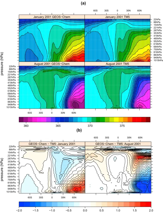
Figure 1. Plot (a) shows simulated CO2in micromoles per mole from GEOS-Chem (left column) and TM5 (right column), averaged zonally and over the
month of January 2001 (top panels) and August 2001 (bottom panels) as a function of latitude and altitude from the simulations described in section 2.2. Differences are shown in plot (b). Both models use a terrain-following sigma vertical coordinate. For simplicity, the y axis shows the 47 GEOS-Chem model levels with approximate pressure levels at sea level.
Figure 2. GEOS-Chem minus TM5 difference in simulated fossil fuel CO2in micromoles per mole, averaged zonally
and over the month of March 2008 as a function of latitude and pressure. Both simulations used CT2016 fossil fluxes. The vertical axis of the plot (b) represents equally spaced pressure levels with the label corresponding to the equivalent sea surface level grid for the sigma terrain-following coordinates. Panel (a) shows the GEOS-Chem minus TM5 difference in pressure-weighted average XCO
2as a function of latitude (solid black line). This is equivalent to the
vertical average of the field shown in panel (b), with the exception that panel (b) is area weighted from a value of one near the equator to zero at the poles. Panel (c) shows the meridional-averaged difference as a function of pressure level. The dashed lines in panels (a) and (c) show the approximate effect of computing XCO
2using an estimated Orbiting
Carbon Observatory-2 (OCO-2) averaging kernel as a function of solar zenith angle and latitude. The blue line in top panel (a) shows the pressure-weighted average of the bottom five model levels. The OCO-2 averaging kernel (AK) is only defined where OCO-2 observations exist; thus, we estimated the AK as a function of latitude and solar zenith angle in order to be able to apply to arbitrary atmospheric columns.
We compare surface fluxes estimated from two numerical experiments in which different observational constraints are assimilated. The first experiment, labeled IS, is one in which only traditional in situ CO2
measurements are assimilated. The second experiment, LN, is one in which 10-s averages of OCO-2 land nadir retrievals of bias-corrected XCO2only are assimilated. These two experiments differ not only in that
there are vastly more XCO2retrievals than in situ measurements but also in the vertical information content
of the observational constraints. In situ measurements are mostly at the surface or within the PBL, whereas XCO2integrates the whole column content of CO2.
3. Results
3.1. CO2Distributions From Forward Simulations 3.1.1. Zonal-Mean Atmospheric CO2Differences
The transport differences between GEOS-Chem and TM5 are evident in the meridional distribution of simulated CO2from the forward simulations described in section 2.2. It is convenient to summarize this
by computing zonal-average “curtains” of CO2. For this comparison, TM5's output is remapped from its
25 level vertical grid to GEOS-Chem's 47 level vertical grid in a manner that conserves column-averaged concentrations. This allows both models to be analyzed at the same time and space resolution.
Figure 3. Similar to Figure 2 but for the sum of all CT2016 nonfossil fuel CO2tracers (land biosphere, fires, and ocean)
for March 2008 and September 2008. Top panel: Black line is full column XCO2, black dotted line is with addition of
OCO-2 averaging kernel, and blue line is the column CO2average for the bottom five model levels.
Figure 1 presents a comparison of the modeled CO2for the total CO2flux (land biosphere net ecosystem
exchange and fire emissions, air-sea CO2flux, and fossil fuel emissions) 12 months (January 2001) and 20
months (August 2001) into the simulation. The models agree reasonably well on the vertical and meridional structure of the CO2distribution, with the differences between the models generally being less than the
common variations seen vertically and seasonally in both models. Both models show similar signatures of vertical and poleward transport of surface CO2exchange from northern midlatitudes. In the boreal winter, when terrestrial photosynthesis is at a minimum and input of CO2from biological respiration and fossil fuel combustion dominates surface exchange, the Northern Hemisphere troposphere has higher CO2than the rest of the atmosphere. In the boreal summer, the same atmospheric zone has the lowest CO2due to surface uptake by terrestrial photosynthesis.
We first analyze the differences in the distribution of the fossil fuel tracer which are shown in Figure 2. Fossil fuel emissions of CO2are always positive and reasonably unchanging over time, reducing
possi-ble complications from covarying surface fluxes and atmospheric transport fields. Analysis of differences between the two models in the fossil fuel tracer shows that the deficit in GEOS-Chem CO2aloft appears immediately in the Northern Hemisphere and at the same time as the surplus of near-surface CO2 over the same area. We conclude that this large difference aloft appears to be from TM5 transporting fossil fuel CO2to the Northern Hemisphere upper troposphere, while GEOS-Chem has stronger north-ward advection and trapping near the surface. Second, by analyzing the fossil fuel tracer many years into the simulation, one can see that a stronger fossil outflow in the low/middle southern latitudes by GEOS-Chem (extending from near surface around 10◦S and extending to about 300 hPa at 40◦S in Figure 2) appears to enter high in the upper troposphere and is also mixed down near the surface. We note that anticorrelated differences between the models in the stratosphere which we speculate are due to differing
Figure 4. Zonal-mean GEOS-Chem minus TM5 differences in simulated XCO2in micromoles per mole. These
Hovmoller plots show the dominant latitude and time differences of simulated XCO
2between the two models. (a)
Summed differences in the land biosphere, fire, and ocean tracers and excludes the fossil fuel tracer. (b) Differences in the fossil tracer alone. (c) The total signal by summing all CO2tracers. The three plots on the left side of the figure show the average difference over the 4 years as a function of latitude, area weighted from a value of 1 near the equator to 0 near the poles. The figure is the same for all three rows with green being the biological, fires, and ocean signal, red being the fossil signal, and black being the total signal.
Figure 5. The 9-year average model-minus-observed residuals of SF6at the
marine boundary layer sites listed in Table S1, arranged by latitude. Results are from two different versions of TM5 with ERA-i meteorology (gold, an earlier version subject to a fault in convective transport; red, a version correcting that fault) and GEOS-Chem using MERRA2 (blue).
mixing characteristics in the upper troposphere-lower stratosphere (UTLS) and stratosphere, since independent research has revealed no significant differences in tropopause height between the MERRA and ERA-i reanalyses used in these models. The strong signals of CO2
dif-ference in the upper layers of the atmosphere at around 88 hPa appear to be tied to a discontinuity in layer pressure thicknesses in the strato-sphere in the TM5 model (see GEOS-Chem and TM5 pressure thick-ness plot in Figure S1). We note that UTLS mixing in the GEOS-Chem model was discussed in detail in a recent model-data comparison paper (Deng et al., 2015) and is a fundamental part of an upcoming paper by Dr. Brad Weir at NASA-GMAO. It will not be discussed further here. Interpretation of the vertical differences in the forward runs of the biolog-ical tracer, which comprises terrestrial biologbiolog-ical emissions including fire and air-sea gas exchange, is made more difficult by the fact that the flux signal changes intensity and sign seasonally while being distributed more broadly in latitude than fossil fuel emissions. This seasonal flux variabil-ity is also correlated with transport mechanisms having strong seasonal variability, such as PBL mixing and the strength of midlatitude storm systems. It is clear from Figure 3 that the source of the strong seasonal variations seen in Figure 1 is the seasonal nature of carbon exchange in the terrestrial biosphere. We note that the dominant differences appear in the Northern Hemisphere both at the surface and aloft and aloft in the lower latitudes of the Southern Hemisphere.
3.1.2. Column-Averaged XCO2Differences
As atmospheric inverse models begin to assimilate satellite-retrieved CO2 information, it is vital to see how the transport differences between these two models are manifested in vertically integrated XCO2. To simulate XCO2as estimated by OCO-2, three-dimensional CO2mixing ratio fields from TM5 are first
con-servatively remapped to the GEOS-Chem horizontal grid, using the Climate Data Operators (Schulzweida, 2018). Column-averaged XCO2from each model is then created as the vertical weighted average, in which
the layer CO2mole fractions are weighted by the layer pressure thicknesses of each model. For analysis here,
XCO2is then averaged zonally.
A latitude by time plot of the differences in XCO2 between TM5 and GEOS-Chem (Figure 4) shows clear seasonal and meridional patterns. There are distinct regime changes in the XCO2differences around 50◦N, the equator, and 50◦S in all panels of the figure.
Fossil fuel CO2differences are easier to interpret than the other CO2tracers since its emissions are always
positive and with relatively minor trends and seasonality. In Figure 4b one can see that GEOS-Chem manifests a deficit of fossil fuel CO2in the northern midlatitudes compared to TM5. This latitude band cor-responds with the zones of the largest anthropogenic emissions from North America, Europe, and Asia. It appears that GEOS-Chem moves fossil fuel CO2out of this source region more rapidly than TM5 does. This results in more simulated CO2in the southern midlatitudes as well as more CO2in the lower vertical levels in the high northern latitudes. The vertical distributions leading to these features are revealed by Figure 2. For instance, the GEOS-Chem excess of fossil fuel CO2in the Southern Hemisphere is concentrated in the upper atmosphere, suggesting a more rapid interhemispheric transport at upper levels in GEOS-Chem compared to TM5. In the Northern Hemisphere high latitudes, GEOS-Chem manifests an excess of fossil fuel CO2near
the surface, counterbalanced by a deficit aloft, resulting in a smaller average difference in the column. 3.2. Meridional Gradients of Surface SF6
Simulated minus-observed residuals of SF6for the two models are shown in Figure 5. These are 9-year
aver-ages at the stations listed in Table S1. This observational constraint involves surface concentrations of SF6
measured during background conditions in the marine boundary layer, away from immediate continental influences.
Earlier versions of TM5 manifested unrealistically high meridional gradients of surface SF6(Patra et al.,
2011; Peters et al., 2004). This earlier TM5 transport is shown in Figure 5 with gold symbols. That model ver-sion manifests an excess of SF6in the Northern Hemisphere and a deficit in the south. After almost a decade
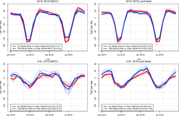
Figure 6. Flux inversion monthly fluxes from the Orbiting Carbon Observatory-model intercomparison project
partitioned by transport model and latitude band. Thin blue lines represent GEOS-Chem models, and thin red lines are TM5 models. Thick blue and red lines represent the ensemble mean for GEOS-Chem and TM5 models, respectively. Upper panels are for fluxes integrated across 45◦N to the north pole, and lower panels represent fluxes integrated from the equator to 45◦N. Left panels show results for inversions assimilating traditional in situ CO2measurements and right panels for inversions assimilating Orbiting Carbon Observatory-2 land nadir retrievals of XCO
2.
TM5 based on Tiedtke (1989) was not representing the vertical mass fluxes of the parent ECMWF model. By this time, however, the ERA-i reanalysis had begun archiving these convective mass fluxes and became pos-sible to apply them directly in TM5 instead of rediagnosing convective transport within the daughter model (Krol et al., 2017; Tsuruta et al., 2017). This “convection fix” (red symbols in Figure 5) almost completely removed the excessive interhemispheric gradient of surface SF6manifested by the earlier TM5 configuration. The convection fix in TM5 had a direct impact on CO2fluxes estimated in CarbonTracker, which uses TM5
as a transport model. In the CT2013 release of CarbonTracker using the faulty convective transport, North-ern Hemisphere land regions were estimated to represent a sink of 2.4 PgC/year. A revised CarbonTracker version using TM5 transport with the convection fix, CT2013B, reduced this sink estimate to 1.8 PgC/year. Oceanic and Southern Hemisphere land fluxes around the world were reapportioned by this change, but this 25% decrease in the estimated Northern Hemisphere land sink was the most significant effect. This provides a quantifiable linkage between the impacts of transport error and inferred surface CO2flux.
GEOS-Chem transport manifests no apparent bias in surface SF6south of about 30◦N (blue symbols in
Figure 5). Poleward of the northern midlatitudes, however, there appears to be an excess of simulated SF6
at the surface, increasing to a maximum in Arctic latitudes. As with CO2, the significant sources of SF6are
estimated to be in the northern midlatitudes (European Commission, 2011), so we infer that there is some anomalously strong meridional transport northward from these latitudes in GEOS-Chem in preference to vertical transport. We again emphasize that due to the constraints of the observations, we can only conclude that an anomalously strong signal of SF6is seen with GEOS-Chem near the surface in this analysis and it is unknown what kind of errors might exist aloft for either model.
3.3. Impacts of Transport Differences on Inferred Surface Fluxes
The OCO-2 MIP (section 2.4.4) includes three inverse models using TM5 and four inverse models using GEOS-Chem. While these small sample sizes preclude robust statistical conclusions, we find differences in inversely derived surface fluxes. These flux differences are consistent with transport differences found from the forward simulations of CO2and SF6.
3.3.1. A Distinct Signature in Flux Seasonality
The transport differences seen in the forward CO2and SF6simulations suggest that we should be able to see
a difference in the amplitude of the seasonal cycle of optimized fluxes from approximately 45◦N to 90◦N and from the equator to 45◦N. It was already shown that GEOS-Chem sees a surplus relative to TM5 of surface CO2and XCO2during boreal winter north of about 45
◦N and a deficit of these same quantities during boreal
summer in the same zone. As argued by Stephens et al. (2007), GEOS-Chem inversion systems need to esti-mate smaller (larger) flux seasonality north (south) of 45◦N to agree with available observational constraints. Therefore, we would expect that GEOS-Chem inverse models would retrieve a smaller seasonal cycle at high northern latitudes and a larger seasonal cycle at tropical and northern midlatitudes. In Figure 6, we plot the seasonal cycles of total fluxes for these two bands by month for each inversion contribution and calculate the average and standard deviation of the ranges for each of the transport families. Figure 6 reveals that the peak-to-peak amplitudes of monthly optimized fluxes for models utilizing GEOS-Chem tend to estimate a weaker seasonal cycle in CO2flux in the higher latitudes of the Northern Hemisphere and a stronger sea-sonal cycle in the lower latitudes compared to TM5 models. This is true in both the IS experiment, in which models assimilate traditional in situ CO2measurements, and in the LN experiment, in which OCO-2 land nadir model retrievals of XCO2are assimilated. These differences are small, and there is a great deal of scatter among models due to inversion methods and configuration details, so they are not statistically significant. In the 45◦N to 90◦N latitude band, there is one GEOS-Chem model with a particularly weak seasonal cycle in the IS inversion and a different one with a particularly weak seasonal cycle in the LN inversion. Removing each of these simulations from those particular comparisons, which still leaves three GEOS-Chem and three TM5 models, reduces the difference in peak-to-peak seasonal cycle between the transport model groups but still leaves a 5–10% difference in general in the 45–90◦N band.
Noisy as they may be, these results are qualitatively consistent with transport differences identified from the forward simulations of CO2and SF6. From those simulations we hypothesize that GEOS-Chem moves
surface emissions out of the northern midlatitudes more quickly than TM5. In a flux inversion context, this means that the land biosphere uptake signal in Northern Hemisphere summer is being removed from its source region more quickly in GEOS-Chem. Hence, that model would require greater uptake in its optimized fluxes over that region to agree with the observational constraints. Conversely, north of 45◦N, GEOS-Chem has imported more of that signal of land uptake and thus requires a smaller summer land sink to agree with observations.
Previous results suggest that we could expect IS optimized fluxes to be more sensitive to transport errors than LN optimized fluxes (Basu et al., 2017; Rayner & O'Brien, 2001). The stronger seasonality differences here under in situ constraints seem to support this.
3.3.2. Impact on Estimates of Annual-Mean Flux
Using vertical profile data from aircraft observations, Stephens et al. (2007) found that inversion models which preferentially “trapped” surface flux signals close to the ground-derived surface fluxes with a weaker seasonal amplitude. In terms of an annual-mean effect, these models simulated a larger carbon sink over northern midlatitudes. It is true that seasonal correlations of surface flux and weather-driven transport mechanisms should drive the amplitude of flux seasonality in inverse models. To explain the annual-mean sink, however, we must also acknowledge that the CO2from fossil fuel combustion at the same latitudes is
subject also to these transport differences. The more stagnant of the two models will retain anomalous fossil fuel CO2in the northern midlatitudes. Since most inverse models do not optimize fossil fuel emissions, the
stagnant model must be driven to estimate extra uptake in its midlatitude land and ocean fluxes to correct for this extra CO2. The more northern region sees an opposite effect, and there the more stagnant model
would have to simulate less of a land-ocean sink to agree with observations.
This is largely what we see in both high-latitude bands, 45◦N to 90◦N and 45◦S to 90◦S (Figure 7). Using in situ data, the median annual drawdown between 45◦N and 90◦N in the GEOS-Chem-based systems is −1.95 PgC/year (range: −2.39 to −1.06), while the three TM5-based frameworks have a median annual sink of −1.73 PgC/year, 11% less. The land nadir data produce weaker overall sinks, but larger differences, with the GEOS-Chem-based frameworks producing a median sink of −1.34 PgC/year (range: −1.67 to −0.83) and the TM5-based frameworks producing a median sink of −0.74 PgC/year (range: −1.09 to −0.35), 45% less. This difference in high latitudes reverses sign as we move south, with GEOS-Chem based frameworks having a much stronger source of CO2in the 0◦N to 45◦N zonal band, consistent with the large deficit of CO2seen
Figure 7. Annual flux average (2015–2016) from Orbiting Carbon Observatory-2 model intercomparison project suite.
IS refers to inversions constrained with traditional in situ observations, and LN refers to inversions constrained with XCO
2retrievals from Orbiting Carbon Observatory-2 in its land nadir observing mode. The box and whiskers plot
shows a box which roughly approximates the first and third quartiles of the data and whiskers which extend to the most extreme data point which is no more than 1.5 times the length of the box away from the box.
in Figure 4. The difference between median annual fluxes is 0.98 PgC for the IS inversions and 1.72 PgC for sthe LN inversions. The surplus of CO2in Figure 4 in the 0–45◦S band would seem to infer; we might
find a corresponding relative sink there in the flux results. However, the fluxes are similar between the two transport models in the equator to 45◦S band, leaving the GEOS-Chem inversions with a weaker integrated global sink relative to TM5. We note that this is consistent with the simulations shown in Basu et al. (2017), and although the exact reasons for this are unknown, we suspect that the 2-year duration of the simulations may not be long enough to ensure agreement on the global sink to the levels desired.
We would be remiss not to present a word of caution. It is often tempting to try to “invert the concentrations by eye”, that is, estimate local surface fluxes which would match the residual annual differences in XCO
2by
zonal bands. There are instances where this approach appears to work well, for example, the correspondence between the large deficit of CO2in the northern midlatitudes seen in Figure 4c and the OCO-2 annual flux differences shown in Figure 7. However, this same approach does not appear to work in the southern midlatitudes where we see an excess of CO2(aloft) in Figure 4. Furthermore, it has been shown in previous
studies (Chan et al., 2008; Denning et al., 1996) that significant meridional gradients in surface CO2can arise
from an annually balanced model through complex covariances between flux and transport, often termed “rectifier effects.” The rectifier effect body of work has not been extended to column-averaged satellite data. However, it would seem to make one cautious when making inferences about surface CO2fluxes based upon
XCO2 differences, particularly with respect to biological fluxes which certainly would covary in time with
both PBL mixing depths and mid-latitude eddy mixing strength.
3.4. Quantification of Impact of Transport Error via Direct Atmospheric Inversion of Transport Differences
Our investigation on the effect of transport differences on CO2surface flux inversions has been largely indi-rect up to this point. In an attempt to more diindi-rectly quantify transport difference impacts, we use a simple flux inversion framework to directly calculate the flux perturbation corresponding the XCO2differences in
Figure 4c. These XCO2differences are first averaged by month and 5
◦latitude band. This particular binning
Figure 8. The effect of monthly average climatological transport bias on a simple inversion of XCO2. The black line is
the monthly four-model mean GEOS-Chem minus three-model mean TM5 flux difference from the LN experiment of the Orbiting Carbon Observatory-2 model intercomparison project. The red line is the result of inverting a smoothed version, by month and 5◦latitude band, of the XCO2difference plotted in Figure 4, using the Schuh GEOS-Chem based inversion framework. “Inversion adjustment” results are smoothed with 3-month boxcar average. Results are in Teragrams carbon per day.
from the diurnal or synoptic cycles. We then generate simulated bias observations at the locations of the 10-s average OCO-2 v7 product, replacing the OCO-2 v7 retrieval with a corresponding bias estimate from that latitude by month bin. We then assimilate this perturbation with a GEOS-Chem-based flux inversion framework, to estimate the effect on surface CO2fluxes. This result is dependent upon the transport model (GEOS-Chem) and inversion method chosen.
The inversion method used here is a batch synthesis inversion (Enting, 2002) where the Jacobian, that is, the matrix of sensitivities of XCO2to linear scalings of the CO2fluxes, is built by running CO2pulses through
GEOS-Chem and measuring the effect on XCO2in places where OCO-2 can measure. The pulses are com-posed of harmonic functions of respiration and gross primary production, for example, seven forward tracers for each of gross primary production and respiration, for each of three different years (2014, 2015, and 2016), for each of 11 TRANSCOM land regions http://transcom.project.asu.edu/ transcom03_protocol_basisMap. php, and each of 24 possible plant functional types. This forms a land flux Jacobian matrix of size approx-imately (3*7*2*11*24) by “number of observations.” The ocean sensitivities are captured in an augmented Jacobian but constrained very tightly to the prior. It is important to note that all corrections to XCO2are
essen-tially attributed to land fluxes in this inversion, whereas variability in prior uncertainty on the ocean fluxes in the broader OCO-2 MIP may lead to differences between this inversion and the TM5 and GEOS-Chem suite averages. More details on methodology will be available in an upcoming manuscript. We will refer to this inversion as the “PSEUDO” inversion run. Results are shown in Figure 8.
The resulting flux perturbation is largely as one would expect, providing local time-space fluxes which would be necessary to create the XCO
2differences in Figure 4. The annual seasonal cycle of CO2to the north of
45◦N is modified by a seasonally varying flux signal on the order of approximately 5 TgC/day, while the annual seasonal cycle of CO2to the south of 45◦N is modified by approximately the same amount but with
a reversed seasonal cycle. We provide the monthly average difference between the GEOS-Chem and TM5 suites of Land Nadir OCO-2 XCO2inversion models (noted in section 2.4.4) as reference. There is reasonably good agreement in terms of the correlation between the suite-wide difference and the PSEUDO estimate although there are some indications of a 1- to 2-month phase shifting of the signal. One would not expect perfect agreement here because of the inversion suite's additional differences in inversion setup and a priori fluxes. However, there is a significant difference in amplitude between the PSEUDO and the suite-wide differences. The PSEUDO flux estimate represents an adjustment of 7% and 12% on the seasonal cycles of the 45◦N to 90◦N and equator −45◦N bands respectively, about half of what we see in the inversion suite. We also note that the offset in the mean annual flux retrieved in Figure 8b is likely due to the fact that this particular inversion is only correcting land fluxes and unable to correct fossil fuel emissions or ocean fluxes in order to mimic the portion of the transport difference associated with fossil CO2shown in Figure 4b or ocean fluxes which are embedded in Figure 4a.
An analysis of posterior XCO2residuals of the PSEUDO fit shows temporally and spatially correlated
pos-terior residuals, potentially indicating that the temporal and spatial frequencies of the pulses used as a basis for flux correction in this particular inversion scheme may be too coarse to capture sharp changes across time and space and are hence an overly smoothed flux estimate with weaker amplitude in time than the truth.
4. Discussion and Path Forward
It has been shown that GEOS-Chem and TM5 manifest significant large-scale differences in their distribu-tion of passive trace gases. While the causes of these differences are not immediately obvious, four potential suspects stand out and all are associated with the modeling of vertical motion.
The likely mechanisms driving differences in transport between GEOS-Chem and TM5 all have some sea-sonal variability. However, qualitative explanations for both the forward simulation differences of CO2and
SF6and also the differences in inversely modeled optimized fluxes do not require a strong seasonal
compo-nent of the transport difference. While seasonal differences in transport certainly exist, the significant effects of that transport difference can be explained without relying on seasonality.
The likely mechanisms driving differences in transport between GEOS-Chem and TM5 all have some sea-sonal variability. However, qualitative explanations for both the forward simulation differences of CO2and SF6and also the differences in inversely modeled optimized fluxes suggest the strong seasonal variations in the model differences arise more as a function of the seasonality of the underlying flux field than the sea-sonality of transport differences between the models. Many unfamiliar with trace gas advection studies of CO2may find this surprising.
The simplest description of the phenomenon from the current results is that GEOS-Chem has some combi-nation of vertical and meridional motion that more quickly ventilates the northern midlatitudes compared to TM5. This vigorous meridional transport in GEOS-Chem moves the strong surface flux signals of the lower midlatitudes, around 30◦N to 45◦N, to northern boreal latitudes and also to the south more quickly than TM5. The fates of those two branches of meridional mixing are very different. Tracers moved more quickly to the south get entrained in the more vertically diffusive regime of vigorous (sub)tropical convec-tion and become quickly mixed through a large volume of air associated with Hadley circulaconvec-tion and also thus mixed into the Southern Hemisphere troposphere. Tracers that moved more quickly to the north out of the northern midlatitudes are instead subject to being entrained into midlatitude synoptic weather pat-terns and the Ferrell circulation. Anomalous transport into this northern branch might be strongly evident in concentration differences because it is mixing into a much smaller volume of air.
4.1. Deep Convection and Interhemispheric Exchange
The strong differences we see in interhemispheric mixing, as evidenced by the fossil fuel signal could be related to differences in the model characterizations of deep and/or shallow convection. The role of deep convection in the tropics and its relationship with the strength of interhemispheric mixing is complicated; nevertheless, it is thought that increasing the strength of tropical convection should impede interhemi-spheric transport in general (Bowman, 2006; Erukhimova & Bowman, 2006). Yu et al. (2018) showed that the averaging of meteorological fields necessary to use GEOS-Chem produces weakened tropical convection relative to the parent GEOS-5 model. Increasing the strength of tropical convection in GEOS-Chem would
likely reduce the interhemispheric gradient we see in Figure 4 by both reducing the excess CO2in the SH
as well as the deficit in the NH lower latitudes. The main hypothesis of Yu et al. (2018) is that the regrid-ding to coarse resolutions of increasingly higher-resolution native reanalysis products such as MERRA2, which is archived from 0.25◦data assimilation products, can result in transport biases. This can lead to a potential loss of resolved convection and an overall low bias in the convective fluxes used in GEOS-Chem. In contrast, TM5 meteorology is regridded from a 80-km meteorological product where presumably more convection is parameterized instead of being directly represented. We do note that ERA-i will be replaced in the near future with ERA5 which will have a resolution of about 31 km, which is much closer to that of MERRA2. Yu et al. (2018) proposed code updates to GEOS-Chem, not yet implemented, which redi-agnose convection from the coarse-averaged meteorology fields, as opposed to directly inputting parent model convective mass fluxes. We expect that this will provide us with one possible path forward to explore the differences.
4.2. PBL Mixing and Vertical Advection/Diffusion in Troposphere
While tropical convection likely represents the strongest source of differences between the models in an inte-grated sense, that is, hemispheric carbon burdens, there are other areas where the models show coherent differences. Vertical diagnostic plots and the SF6analysis showed trapping in the GEOS-Chem model where
the near-surface northern high-latitude areas saw a stronger signal of the local surface flux contribution, that is, positive for fossil fuels and negative for photosynthesis. PBL mixing and the modeling of entrain-ment near the PBL top are likely areas where models may differ. Furthermore, vertical velocities are often calculated diagnostically by chemical transport models as a function of horizontal divergence. Potential problems from this approach, in combination with a loss of information in time-space-averaged reanalysis fields, could certainly play a role in the differences we see in vertical mixing between the models. While we do not investigate vertical advection differences between the models, we acknowledge its potential impor-tance to the differences shown here. We note that the accuracy of GEOS-Chem in addressing this process is under investigation by Dr. Dylan Jones at the University of Toronto. Due to the difficult nature of compar-ing models with quite different vertical turbulent mixcompar-ing schemes in the PBL and the free troposphere, we refer readers to Dr. Jones's ongoing research.
4.3. Slant Convection Processes Across Midlatitude Frontal Boundaries
Local mixing differences in the model due to differences in PBL mixing and vertical advection/diffusion are likely suspects to generate the differences we are seeing in the northern middle/high latitudes. However, it is also interesting to note that the north-south locations of the sign changes in the differences seen in Figure 4, as well as the strongest surface gradients in the differences in Figure 3, are approximately located over the intertropical convergence zone and the two midlatitude storm tracks. Furthermore, there is evidence in these plots of the subtle north-south movement of these features seasonally, likely matching the weakening and poleward movement of the midlatitude storm track in the summer and the subsequent strengthening and equatorward movement in the winter. These results would seem to suggest potential differences in the modeling and resolving of midlatitude frontal systems in isolation or in addition to potential local mixing effects, for example, vertical advection or PBL mixing and venting.
4.4. Upper Tropospheric/Lower Stratospheric Exchange
Lastly, we note that care must be taken to condition this future research upon unknown differences in UTLS mixing between the models. It has been well documented that UTLS mixing in recent versions of GEOS-Chem is likely too strong (Eastham et al., 2014) and simulations of O3and CO2show increasing
difficulties as one heads toward the poles (Deng et al., 2015; Greenslade et al., 2017).
We have conducted simulations of CO2and SF6in two widely used chemical transport models driven by state-of-the-art reanalysis products from ECWMF and NASA-GMAO and using identical surface fluxes in both models. Differences in tracer distributions are a convolution of the transport differences and the struc-ture of the underlying emissions. Our intention was to view the transport difference in the space of realistic fluxes. For carbon dioxide, these fluxes are dominated by increasing fossil fuel emissions and the season-ality of biological photosynthesis and respiration in the northern midlatitudes. The particular choice of CO2flux is less important than the fact that the flux field is a reasonable representation of seasonally and
interannually varying fluxes.
The resulting differences in our model simulations clearly show coherent structures in time and space. For SF6, whose modeled emissions have no seasonal variability, GEOS-Chem manifests excess surface
concen-trations north of about 45◦N with no obvious time dependence. This should be similar to the behavior of the fossil fuel CO2tracer, which has only modest seasonality. Temporal patterns in XCO2differences corre-spond to the cycle of northern midlatitude biological CO2fluxes, while spatial patterns appear to correspond to the positioning of strong meridional mixing features, in particular, the midlatitude storm tracks and the intertropical convergence zone. We show that these differences are significant enough to manifest them-selves in atmospheric flux inversion results with (1) an explicit inversion of the XCO2differences, as well
as (2) an analysis of the seasonal amplitude/range and annual fluxes of the current suite of OCO-2 CO2
flux inversion results. When compared to the mean seasonal cycles of CO2flux produced by atmospheric
inversions, the transport difference amounts to an error of approximately 10–15% of the mean seasonal cycle. We also find significant annual flux differences between the inversions run with TM5 and those run with GEOS-Chem and that those differences corresponded roughly with the annually averaged differences on large scales, with the exception of a difference aloft in the southern hemisphere low latitudes which appears to drive a difference in the estimated annual global carbon sinks (as discussed in section 3.3.2). The exact transport mechanisms responsible for the concentration differences between the forward runs, the general correspondence with annual flux inversion results in the Northern Hemisphere, and the lack of correspondence in portions of the Southern Hemisphere are still under investigation.
References
Ballantyne, A. P., Alden, C. B., Miller, J. B., Tans, P. P., & White, J. W. C. (2012). Increase in observed net carbon dioxide uptake by land and oceans during the past 50 years. Nature, 488(7409), 70–72. https://doi.org/10.1038/nature11299
Barnes, E. A., Parazoo, N., Orbe, C., & Denning, A. S. (2016). Isentropic transport and the seasonal cycle amplitude of CO2. Journal of Geophysical Research: Atmospheres, 121, 8106–8124. https://doi.org/10.1002/2016JD025109
Basu, S., Baker, D. F., Chevallier, F., Patra, P. K., Liu, J., & Miller, J. B. (2017). The impact of transport model differences on CO2surface flux estimates from OCO-2 retrievals of column average CO2. Atmospheric Chemistry and Physics Discussions, 18, 7189–7215. Bey, I., Jacob, D. J., Yantosca, R. M., Logan, J. A., Field, B. D., Fiore, A. M., et al. (2001). Global modeling of tropospheric chemistry with
assimilated meteorology: Model description and evaluation. Journal of Geophysical Research, 106(D19), 23,073–23,095.
Bosilovich, M. G. (2015). Technical report series on global modeling and data assimilation, volume 43 MERRA-2: Initial evaluation of the climate. NASA-GMAO. Retrieved from https://gmao.gsfc.nasa.gov/pubs/docs/Bosilovich803.pdf
Bowman, K. P. (2006). Transport of carbon monoxide from the tropics to the extratropics. Journal of Geophysical Research, 111, D02107. https://doi.org/10.1029/2005JD006137
Chan, D., Ishizawa, M., Higuchi, K., Maksyutov, S., & Chen, J. (2008). Seasonal CO2rectifier effect and large-scale extratropical atmospheric transport. Journal of Geophysical Research, 113, D17309. https://doi.org/10.1029/2007JD009443
Crowell, S., Baker, D., Schuh, A., Basu, S., Jacobson, A. R., Chevallier, F., & Sweeney, C. (2019). The 2015-2016 carbon cycle as seen from OCO-2 and the global in situ network. Atmospheric Chemistry and Physics Discussions. https://doi.org/10.5194/acp-2019-87 Deng, F., Jones, D. B. A., Walker, T. W., Keller, M., Bowman, K. W., Henze, D. K., et al. (2015). Sensitivity analysis of the potential impact of
discrepancies in stratosphere-troposphere exchange on inferred sources and sinks of CO2. Atmospheric Chemistry and Physics, 15(20), 11,773–11,788.
Denning, A. S., Collatz, J. G., Zhang, C., Randall, D. A., Berry, J. A., Sellers, P. J., et al. (1996). Simulations of terrestrial carbon metabolism and atmospheric CO2in a general circulation model. Part 1: Surface carbon fluxes. Tellus, 48B, 521–542.
Denning, A. S., Holzer, M., Gurney, K. R., Heimann, M., Law, R. M., Rayner, P. J., et al. (1999). Three-dimensional transport and concentration of SF6. a model intercomparison study (TransCom 2). Tellus, 51B, 266–297.
Dentener, F. (2003). Interannual variability and trend of CH4lifetime as a measure for OH changes in the 1979–1993 time period. Journal of Geophysical Research, 108(D15), 4442. https://doi.org/10.1029/2002JD002916
Eastham, S. D., Weisenstein, D. K., & Barrett, S. R. H. (2014). Development and evaluation of the unified tropospheric-stratospheric chemistry extension (UCX) for the global chemistry-transport model GEOS-chem. Atmospheric Environment, 89, 52–63.
Eldering, A., O'Dell, C. W., Wennberg, P. O., Crisp, D., Gunson, M. R., Viatte, C., et al. (2017). The orbiting carbon observatory-2: First 18 months of science data products. Atmospheric Measurement Techniques, 10(2), 549–563.
Enting, I. G. (2002). An empirical characterisation of signal versus noise in CO2data. Tellus Series B-Chemical and Physical Meteorology, 54(4), 301–306.
Erukhimova, T., & Bowman, K. P. (2006). Role of convection in global-scale transport in the troposphere. Journal of Geophysical Research, 111, D03105. https://doi.org/10.1029/2005JD006006
European Commission (2011). Emission database for global atmospheric research (edgar), release version 4.2. http://edgar.jrc.ec.europa.eu Greenslade, J. W., Alexander, S. P., Schofield, R., Fisher, J. A., & Klekociuk, A. K. (2017). Stratospheric ozone intrusion events and their
impacts on tropospheric ozone in the Southern Hemisphere. Atmospheric Chemistry and Physics, 17(17), 10,269–10,290.
Houweling, S., Dentener, F., & Lelieveld, J. (1998). The impact of nonmethane hydrocarbon compounds on tropospheric photochemistry. Journal of Geophysical Research, 103(D9), 10,673–10,696.
Krol, M., de Bruine, M., Killaars, L., Ouwersloot, H., Pozzer, A., Yin, Y., et al. (2017). Age of air as a diagnostic for transport time-scales in global models. Geoscientific Model Development Discussions, 11, 3109–3130. https://doi.org/10.5194/gmd-2017-262
Krol, M., Houweling, S., Bregman, B., van den Broek, M., Segers, A., van Velthoven, P., et al. (2005). The two-way nested global chemistry-transport zoom model TM5: Algorithm and applications. Atmospheric Chemistry and Physics, 5(2), 417–432.
Lee, M., & Weidner, R. (2016). Jpl publication 16-4: Surface pressure dependencies in the GEOS-chem adjoint system and the impact of the GEOS-5 surface pressure on CO2model forecast. Jet Propulsion Laboratory California Institute of Technology Pasadena, California. Levin, I., Naegler, T., Kromer, B., Diehl, M., Francey, R. J., Gomez-Pelaez, A. J., et al. (2010). Observations and modelling of the global
distribution and long-term trend of atmospheric 14 CO2. Tellus B, 62B(1), 26–46.
Lin, S.-J., & Rood, R. B. (1996). Multidimensional flux-form semi-lagrangian transport schemes. Monthly Weather Review, 124, 2046–2070.
Acknowledgments
Author contributions as follows: A. S. performed the GEOS-Chem CO2 simulations, inverse model analysis, comparisons to CT2016 mole fractions; wrote the manuscript; and performed analysis of results. A. J. was responsible for producing CT2016, conducting the SF6simulations in TM5 and GEOS-Chem, and helping to write the manuscript. B. W. and S. B. were an integral part of the manuscript discussions. OCO-2 L4 inversions results were provided by K. B., J. L., L. F., F. D., S. C., A. S., and A. J. Funding for work came from NASA via funded proposals of A. S., A. J., S. D., and K. D. Specifically, OCO-2 Science Team project (grant NNX15AG93G to Colorado State University and NNX12AP91G to the University of Colorado) and the Atmospheric Carbon and Transport (ACT)-America project, a NASA Earth Venture Suborbital 2 project funded by NASA's Earth Science Division (NNX15AG76G to Penn State, NNX15AJ07G to Colorado State University, and NNX15AJ06G to the University of Colorado). Results, analysis, and current publications related to the underlying atmospheric inversion models are available at their website (https://www.esrl.noaa.gov/ gmd/ ccgg/OCO2/). We also thank Daniel Jacob's group at Harvard University for feedback and support with the GEOS-Chem model.
Maiss, M., & Brenninkmeijer, C. A. (1998). Atmospheric sf6: Trends, sources, and prospects. Environmental Science & Technology, 32(20), 3077–3086.
Masarie, K. A., & Tans, P. P. (1995). Extension and integration of atmospheric carbon dioxide data into a globally consistent measurement record. Journal of Geophysical Research, 100(D6), 11,593–11,610.
NOAA Earth System Research Laboratory, G. M. D. (2016). Cooperative global atmospheric data integration project (2016). Multi-laboratory compilation of atmospheric carbon dioxide data for the period 1957-2015, obspack co2 1 globalviewplus v2.1 2016-09-02. https://doi. org/10.15138/g3059z
Parazoo, N. C., Denning, A. S., Berry, J. A., Wolf, A., Randall, D. A., Kawa, S. R., et al. (2011). Moist synoptic transport of CO2along the mid-latitude storm track. Geophysical Research Letters, 38, L09804. https://doi.org/10.1029/2011GL047238
Patra, P. K., Houweling, S., Krol, M., Bousquet, P., Belikov, D., Bergmann, D., et al. (2011). TransCom model simulations of CH4and related species: Linking transport, surface flux and chemical loss with CH4variability in the troposphere and lower stratosphere. Atmospheric
Chemistry and Physics, 11(24), 12,813–12,837.
Peters, W., Jacobson, A. R., Sweeney, C., Andrews, A. E., Conway, T. J., Masarie, K., et al. (2007). An atmospheric perspective on North American carbon dioxide exchange: CarbonTracker. Proceedings of the National Academy of Sciences of the United States of America, 104, 18,925–18,930. https://doi.org/10.1072/pnas.07089861074
Peters, W., Krol, M. C., Dlugokencky, E. J., Dentener, F. J., Bergamaschi, P., Dutton, G., et al. (2004). Toward regional-scale modeling using the two-way nested global model TM5: Characterization of transport using SF6. Journal of Geophysical Research, 109 D19314. https://doi.org/10.1029/2004JD005020
Peylin, P., Law, R. M., Gurney, K. R., Chevallier, F., Jacobson, A. R., Maki, T., et al. (2013). Global atmospheric carbon budget: Results from an ensemble of atmospheric CO2inversions. Biogeosciences, 10(10), 6699–6720.
Philip, S., Johnson, M. S., Potter, C., Genovesse, V., Baker, D. F., Haynes, K. D., & Poulter, B. (2019). Prior biosphere model impact on global terrestrial CO2fuxes estimated from OCO-2 retrievals. Atmospheric Chemistry and Physics Discussions, 1–29. https://doi.org/10.5194/
acp-2018-1095
Ray, E. A., Moore, F. L., Elkins, J. W., Rosenlof, K. H., Laube, J. C., Röckmann, T., et al. (2017). Quantification of the SF6lifetime based on
mesospheric loss measured in the stratospheric polar vortex. Journal of Geophysical Research: Atmospheres, 122, 4626–4638. https://doi. org/10.1002/2016JD026198
Rayner, P. J., & O'Brien, D. M. (2001). The utility of remotely sensed CO2concentration data in surface source inversions. Geophysical Research Letters, 28(1), 175–178. https://doi.org/10.1029/2000GL011912
Rienecker, M. M., Suarez, M. J., Gelaro, R., Todling, R., Bacmeister, J., Liu, E., et al. (2011). MERRA: NASA's modern-era retrospective analysis for research and applications. Journal of Climate, 24(14), 3624–3648.
Schulzweida, U. (2018). Climate data operators (CDO) user guide, version 1.9.3 (Tech. Rep.). Max Planck Institute for Meteorologie. Retrieved from https://code.mpimet.mpg.de/projects/cdo/embedded/cdo.pdf
Stephens, B. B., Gurney, K. R., Tans, P. P., Sweeney, C., Peters, W., Bruhwiler, L., et al. (2007). Weak northern and strong tropical land carbon uptake from vertical profiles of atmospheric CO2. Science, 316(5832), 1732–1735.
Tiedtke, M. (1989). A comprehensive mass flux scheme for cumulus parameterization in large-scale models. Monthly Weather Review, 117(8), 1779–1800.
Tsuruta, A., Aalto, T., Backman, L., Hakkarainen, J., van der Laan-Luijkx, I. T., Krol, M. C., et al. (2017). Global methane emission esti-mates for 2000–2012 from CarbonTracker Europe-CH4 v1.0. Geoscientific Model Development, 10, 1261–1289. https://doi.org/10.5194/ gmd-10-1261-2017
Wunch, D., Wennberg, P. O., Osterman, G., Fisher, B., Naylor, B., Roehl, C. M., et al. (2017). Comparisons of the orbiting carbon observatory-2 (OCO-2) measurements with TCCON. Atmospheric Measurement Techniques, 10(6), 2209–2238.
Yu, K., Keller, C. A., Jacob, D. J., Molod, A. M., Eastham, S. D., & Long, M. S. (2018). Errors and improvements in the use of archived meteorological data for chemical transport modeling: an analysis using GEOS-Chem v11-01 driven by GEOS-5 meteorology. Geoscientific Model Development, 11, 305–319. https://doi.org/10.5194/gmd-11-305-2018