HAL Id: hal-00918414
https://hal.inria.fr/hal-00918414
Submitted on 17 Dec 2013HAL is a multi-disciplinary open access archive for the deposit and dissemination of sci-entific research documents, whether they are pub-lished or not. The documents may come from teaching and research institutions in France or abroad, or from public or private research centers.
L’archive ouverte pluridisciplinaire HAL, est destinée au dépôt et à la diffusion de documents scientifiques de niveau recherche, publiés ou non, émanant des établissements d’enseignement et de recherche français ou étrangers, des laboratoires publics ou privés.
Comparison of free-streaming ELM formulae to a Vlasov
simulation
D. Moulton, W. Fundamenski, Giovanni Manfredi, Sever Adrian Hirstoaga,
David Tskhakaya
To cite this version:
D. Moulton, W. Fundamenski, Giovanni Manfredi, Sever Adrian Hirstoaga, David Tskhakaya. Com-parison of free-streaming ELM formulae to a Vlasov simulation. Journal of Nuclear Materials, Elsevier, 2013, Proceedings of the 20th International Conference on Plasma-Surface Interactions in Controlled Fusion Devices, 438, Supplement, pp.S633-S637. �10.1016/j.jnucmat.2013.01.133�. �hal-00918414�
1
P1-28
Comparison of free-streaming ELM formulae to a Vlasov simulation
D. Moulton*a, W. Fundamenskib, G. Manfredic, S. Hirstoagad D. Tskhakayae
a
CEA, IRFM, F-13108 Saint-Paul Lez Durance, France
b
Imperial College of Science, Technology and Medicine, London, UK
c
Institut de Physique et Chimie des Matériaux, CNRS and Université de Strasbourg, BP 43, F-67034 Strasbourg, France
d
INRIA Nancy Grand-Est and Institut de Recherche en Mathématiques Avancées, 7 rue René Descartes, F-67084 Strasbourg, France
e
Association EURATOM-ÖAW, University of Innsbruck, A-6020 Innsbruck, Austria
Abstract
The main drawbacks of the original free-streaming equations for edge localised mode transport in the scrape-off layer [Fundamenski, PPCF 48(2006)109] are that the plasma potential is not accounted for and that only solutions for ion quantities are considered. In this work, the equations are modified and augmented in order to address these two issues. The new equations are benchmarked against (and justified by) a numerical simulation which solves the Vlasov equation in 1d1v. When the source function due to an edge localised mode is instantaneous, the modified free-streaming ‘impulse response’ equations agree closely with the Vlasov simulation results. When the source has a finite duration in time, the agreement worsens. However, in all cases the match is encouragingly good, thus justifying the applicability of the free-streaming approach.
PSI-19 KEYWORDS: SOL transport modelling, SOL physics, ELM PACS: 52.25.Fi, 52.55.Fa, 52.55.Rk, 52.65.Ff
CORRESPONDING AND PRESENTING AUTHOR ADDRESS: David Moulton, CEA, IRFM, F-13108 Saint-Paul Lez Durance, France.
2 1. Introduction
Edge localised mode (ELM) plasma instabilities will probably be present in future tokamak devices employing high-confinement mode. Due to the large energies contained in ELMs, it is important to understand the physical mechanisms which govern the duration and area over which they spread their energy onto divertor targets. In this regard, the free-streaming model for ELM transport in the SOL (conceived in [1]) has proven useful. It has been successfully used to fit experimental time profiles of the ELM target power on JET and ASDEX Upgrade [2] and on TCV [3]. It has not, however, been properly benchmarked against a numerical kinetic simulation. This is an important step in understanding the validity of the physics assumptions made in the free-streaming model and is the topic of this contribution.
In the original free-streaming model for ELM transport in a flux tube of open field lines [1], all Coulomb forces are ignored. The ion distribution function is assumed to evolve according to the 1d force-free Vlasov equation
where [ ] is the 1d spatial coordinate, is the parallel velocity, is the ion source function and is the connection length. For the initial value case where and
, (1) has solution . Considering an initial Gaussian density profile ⁄ and an initial velocity distribution that is Maxwellian with temperature , this gives
√
where √ is the initial ion thermal speed (typically, the actual values used for and are those associated with the pedestal region, since that is where the ELM originates).
3
Note that this initial value case is identical to the case of an impulse source in time:
. Therefore, is called the free-str aming ‘im uls r s ons ’ ion distribution function. Furthermore, since (1) is linear, the response to an arbitrary source can be found by convolving that source with , i.e. .
In the interest of finding expressions for experimentally measurable quantities, velocity moments of are taken. For the zeroth moment (i.e. the ion density) this gives an analytic expression (see equation (4)). Higher moments, however, must be calculated numerically. If analytic expressions are required for these higher moments, then the limit
can be assumed (it will be shown in section 4 that this assumption has little effect on
the solution at temporal and spatial coordinates of interest). This limit corresponds to a Dirac delta function for the initial density, i.e. √ , so that equation (2) gives
⁄
Taking velocity moments of now yields equations for measurable quantities (such as the ion energy flux density on the targets), as previously given in [1] and [4].
As recognised in [1], the primary drawback of the approach described above is that the role of the electric potential has been ignored. Furthermore, expressions have thus far only been derived for ion quantities and not for electron quantities. In this paper, these two omissions will be accounted for in modified free-streaming equations, justified on the basis of a numerical Vlasov simulation. That simulation is now discussed.
2. Kinetic simulation observations
The code, used for all the simulations presented in this paper, solves the collisionless 1d1v Vlasov equation for electrons and ions, with the electric potential calculated from the
4
Poisson equation. It is described in detail in [4]. The particular simulation analysed in this section is the one presented in section 4.1 of [4]. To allow comparison with the impulse response free-streaming equations, there was no electron or ion source in this initial value simulation. The initial ion and electron densities were set equal:
⁄ , with . The ion and electron velocity distribution functions were initially Maxwellian with equal ion and electron temperatures: . As a result, for both ions and electrons, the initial total number of particles was √ , the initial parallel energy was ⁄ and the initial gyro-energy was . Note that, in fact, has units of particles/unit area, while and have units of energy/unit area. The area here is perpendicular to and all quantities in this 1d model are an average over this area. Note also that there was no interaction between parallel and gyro-motion and the temperature associated with gyration was assumed to remain constant for all time and space, at a value . The mass ratio and ion charge were hydrogenic: ⁄ ,
, and the boundary conditions at the walls were . The actual values of , and are only important in so far as they set the ratio ⁄ , where √ is the initial Debye length at peak density. A value of was used here (Note that although this value of is times larger than for realistic ELM parameters, the solution remained almost unchanged for smaller values [4]).
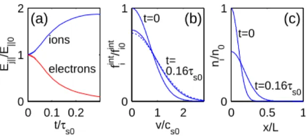
Consider now the transfer of parallel energy from electrons to ions. Figure 1a shows the total parallel energy in the ions and electrons as a function of time for the simulation described above (normalised to ). By time , the electrons donate 71% of their initial parallel energy to the ions (here, ⁄ is the loss time at the initial sound speed,
5
transition in the simulated parallel-integrated ion distribution function, ∫ , from a Maxwellian with standard deviation at to a Maxwellian with standard deviation at (note that in the figure 1b is normalised to its maximum initial value, ). Finally, figure 1c shows ⁄ (as a function of ⁄ ) when and when . These plots demonstrate that the bulk plasma has not moved far from its initial position by the time the aforementioned transition has occurred (in fact, the particle flux density to the target peaks on a timescale , as will be shown in figure 5).
As a result of the timescale for the transition being significantly shorter than the timescale on which the bulk plasma reaches the target, the Maxwellian with standard
deviation can be assumed as an initial condition. After the transition, there is no longer
any parallel energy available in the electrons to accelerate the ions, so that the ions will free stream towards the targets. Thus it is expected that the free-streaming model should be able to account for the electric potential acting on the ions by simply substituting in equation (2) (or in equation (3) if is assumed). This is a key result of this paper. Although this substitution has been made previously in other publications [2, 3, 5], it has never been physically justified by the rapid transition to a Maxwellian with standard deviation observed in a kinetic simulation which corresponds to the free-streaming ELM.
To assess the validity of the assumption that the plasma is collisionless, the timescale on which electrons donate energy to ions should be compared to the shortest collision time, i.e. the electron-ion collision time, given by (Miyamoto 1987), where has units of eV and has units of - . For eV
- , m and hydrogen ions, the initial electron-ion collision time is , whereas
the timescale on which the electrons donate their energy to the ions is . Thus, we expect electron-electron collisions to alter the electron distribution function, but
6
only after the energy transferral has occurred. This is of little importance, since by then the ions carry the majority of the parallel kinetic energy. Nevertheless, since is of a similar order to the electron-to-ion energy transferral time, we accept that electron-electron collisions may play a role in ELM parallel transport and their effect will be investigated in a future study.
3. Modified impulse response free-streaming equations
Making the substitution in (3) and taking appropriate integrals of gives impulse response equations for the total ion number ∫ (∫ ) , the total ion energy ∫ ⁄⁄ (∫ ) , the ion density ∫ , the ion pressure ∫
, the ion flux density ∫
, and the ion energy flux density
∫ . For electrons, the same quantities can
be derived by assuming quasineutrality and using energy conservation. That is, the electron density is assumed to move with the ion density, but electrons have only their gyro-energy since they are assumed to immediately donate all of their parallel energy to the ions. Thus
, , , , and . These
electron equations are a simple but important addition to the free-streaming model, presented here for the first time. The resulting equations, for both ions and electrons, are given in table 1 (note that { } is the species index).
It should be recognised that the equations in table 1 were derived using , i.e. in the limit . Without this assumption, an analytic solution could only be derived from (2) for the density, as follows:
∫ ⁄
⁄ ⁄ ⁄
⁄
7
(note that (4) corresponds to the equation in table 1 when ). For the other quantities, arbitrary values of can be accounted for by convolving the equations in table 1 with an appropriate function representing the initial density distribution in . For an initial Gaussian density, the appropriate function is a normal distribution
( √ ⁄ ) ⁄ , which integrates to unity and therefore conserves the number of particles after convolution. In fact, it will be shown in the next section that accounting for finite in this way has little effect when , compared to the direct application of the equations in table 1.
4. Comparison of impulse responses to simulation
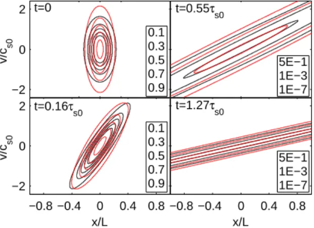
The modified free streaming equations are now compared to the simulation described at the beginning of section 2. To begin, the normalised free-streaming impulse response function for general (i.e. from equation (2) with ) is compared to the simulation. This comparison is shown in figure 2, with the free-streaming distribution function in red and the simulated distribution function in black (both are normalised to
√
⁄ ). By time , the simulation and free streaming model are seen to agree well. Beyond this time there is no longer any parallel energy in the electrons available to accelerate the ions, so that the ions free-stream towards the targets. This is shown by the agreement between the free-streaming model and the simulation at times
and . These times correspond, respectively, to the times required
for the total target energy flux density to reach its maximum and to subsequently fall to ⁄ times its maximum.
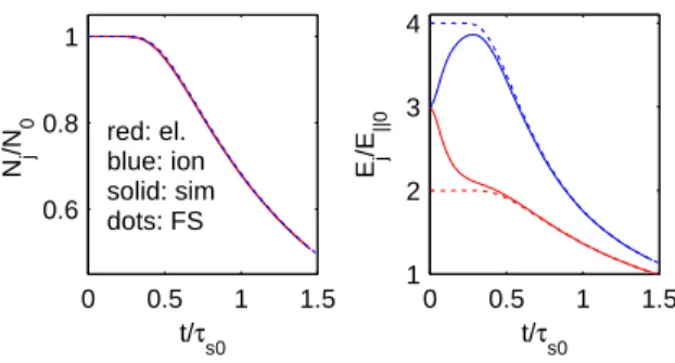
Figure 3 compares and according to the simulation (solid lines) and the free streaming equations in table 1 (dotted lines). Note that these equations are unaltered for general . It is seen that, as a result of quasineutrality, the simulated and align almost
8
exactly for this plasma. Also, the free-streaming equation for (which equals when ) agrees almost perfectly with the simulation. For the energies in the ions and electrons, the free streaming model assumes that all of the parallel energy of the electrons is transferred to the ions as an initial condition, i.e. and . In figure 3, this assumption is seen to be violated in the initial phase of transport, while the transition of parallel energy from electrons to ions is taking place. By time , however, the free-streaming and simulated values for and agree well and afterwards become increasingly well matched as time passes.
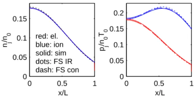
The comparisons between free-streaming values and Vlasov simulation values for and , as functions of ⁄ at time , are shown in figure 4. The free-streaming impulse equations for (i.e. directly from table 1) are shown as dotted lines, while the free-streaming values which account for (i.e. from equation (4) for the species density or using numerical convolution for the species pressure) are shown as dashed lines. Although the accounting for improves the fit with the simulation slightly, the effect is minimal for this value of and the analytic equations in table 1 are sufficient to recover the simulated values to a high degree of accuracy. The electron and ion densities are seen to align almost everywhere, confirming the quasineutrality assumption (except in the sheath region by the targets, where there is the expected drop in electron density).
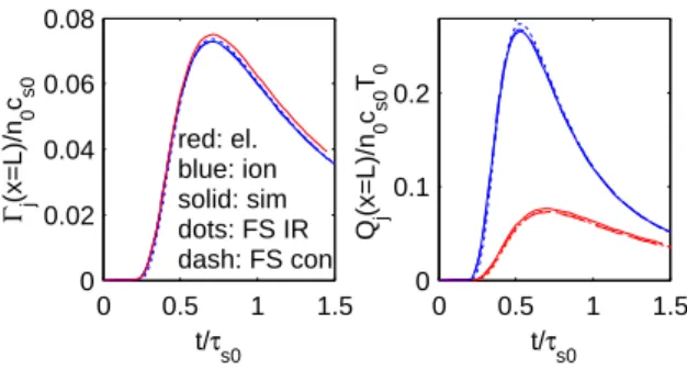
The comparison for the particle and energy flux densities at the targets (as a function of time) is shown in figure 5. Again, the agreement between free-streaming and simulated values is excellent, and the effect of convolution in (to account for ) is small. This level of agreement should be compared to the relatively poor level of agreement shown in figure 1 of [4]. Importantly however, in that figure the free-streaming equations were used with as an initial condition for the standard deviation of the ion distribution function,
9
rather than . In terms of divertor lifetime, the most important quantities are the energy flux densities. It is therefore highly encouraging that such good agreement is found between the simulation and the modified free-streaming equations for these quantities, at least for the impulse response.
It is important to realise that the numerical simulation does resolve a sheath at the wall, while the free-streaming equations ignore it. Thus, the excellent agreement observed for the energy flux densities would not be obtained if the sheath was playing an important role in transferring energy from ions to electrons. For the impulse response simulation, the sheath potential is so small that it has a negligible effect on the electron and ion energy flux densities. This is because the energy transfer from electrons to ions occurs on a timescale shorter than the time on which the bulk plasma reaches the target. Thus, by the time the majority of electrons reach the wall, they no longer have sufficient parallel energy to create a significant sheath potential. This topic will be investigated further in future work.
Finally, consider the timescales on which particles and energy reach the target. The free-streaming equations predict that the particle flux density peaks at ⁄ , while the √
total energy flux density peaks at and subsequently reaches ⁄ times its maximum when .
5. Effect of a time-distributed source
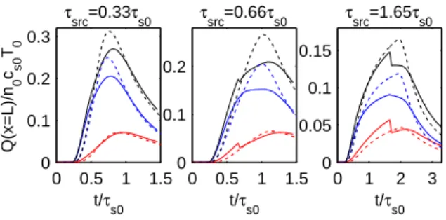
The effect of a time-distributed source in the Vlasov equation, mimicking the flow of particles and energy into the SOL due to an ELM, is now assessed. The source used was as follows:
{ √
10
i.e. a constant source in time starting at , with duration and with the same total number of particles and energy as there were in the initial-value case. The impulse responses
and from table 1 can be convolved with this uniform source function to
yield the following free-streaming equation for the energy flux densities:
⁄ [ ( ) √ (√ )]
where and for electrons, while ⁄ and ⁄ for ions. Also, for both ions and electrons, when and when . Note that accounting for finite by numerically convolving with a normal distribution in has very little effect on equation (6) when .
Figure 6 shows the electron, ion and total energy flux densities to the target according to the Vlasov simulation (solid lines) and according to equation (6) (dotted lines), for three different source durations of , and . The free-streaming solution differs from the simulation most strongly for the case, when the source duration is similar to for the impulse response. For all source durations, however, the agreement between the analytic free-streaming expressions and the simulations is reasonable, especially given the former’s ease of application compared to solving the Vlasov equation numerically. This is particularly true of the total energy flux density (shown in black), which is the most important quantity in terms of divertor lifetime. 6. Conclusions
The free-streaming equations for ion ELM transport with the substitution , and the new free-streaming equations for electron ELM transport, have been shown to agree well with equivalent solutions from a Vlasov simulation, particularly for the impulse response (initial value) case. This important validation adds credence to a model which has
11
already been successfully fitted to existing experimental ELM power loading data [2,3] and justifies its future applicability for predicting the duration of ELM power loading on ITER. The following questions remain, however, and will be the focus of future work. What is the effect of a radially varying connection length on the time profile of the power to the target? Do the predictions made by the free-streaming model agree with the experimentally observed
-dependence of ELM power loading? What is the effect of different impurity concentrations
on the duration of the ELM power load? What sets the transfer time required for electrons to donate their parallel energy to the ions and at what point will this transfer time become long enough that the free-streaming equations break down? What effect do collisions and/or a pre-existing background plasma have on the validity of the free-streaming model? Finally, and most importantly, what will set the duration of the ELM power load on ITER? The results presented here show that the free-streaming model is a physically relevant and easily applicable tool that hopefully can be used to answer these questions.
Acknowledgements
This work was supported by EURATOM and carried out within the framework of the European Fusion Development Agreement. The views and opinions expressed herein do not necessarily reflect those of the European Commission.
References
[1] W. Fundamenski, R. A. Pitts, Plasma Phys. Control. Fus. 48 (2006) 109. [2] T. Eich et al., J. Nucl. Mater. 390-391 (2009) 760.
[3] J. Marki et al., J. Nucl. Mater. 390-391 (2009) 801.
[4] G. Manfredi et al., Plasma Phys. Control. Fus. 53 (2011) 015012
12
[6] D. Tskhakaya et al., J. Nucl. Mater. 390-391 (2009) 335. Figure and table captions
Table 1: Modified free-streaming equations for the total number of particles, total energy, density, pressure, particle flux density and energy flux density. Each quantity is given for ions ( ) and electrons ( ).
Figure 1: (a) Total parallel energy in the ions and electrons as a function of time according to the Vlasov simulation. (b) The parallel-integrated distribution functions when and when , according to the simulation (solid lines). Shown for comparison is the dotted line, which is a Maxwellian with standard deviation . (c) Density profiles when
and when . All figures only shown for positive only due to symmetry of
the solutions about .
Figure 2: Comparison of Vlasov simulation (black) and free-streaming (red) normalised ion distribution functions, ⁄( ⁄√ ), for the initial value case at four different times. At each time, the contour levels (shown in boxes) are the same for simulated and free-streaming plots.
Figure 3: Comparison between the Vlasov simulation (solid lines) and free-streaming equations (dotted lines) for the total number of particles and total energy as a function of time for the initial value case. Electron values are in red, ion values are in blue.
Figure 4: Comparison between the Vlasov simulation and free-streaming model for the density and pressure profiles in space at time . The same colours and line styles are used as for figure 3, with the additional dashed lines accounting for .
13
Figure 5: Comparison between the Vlasov simulation and free-streaming model for the particle and energy flux densities at the target as a function of time. The same colours and line style are used as for figure 4.
Figure 6: Comparison between the Vlasov simulation and free-streaming equation (5) for the energy flux densities at the target as a function of time, due to a uniform ELM source of duration . Plots are shown for three different values of . Electron values are in red, ions values in blue and total values in black. Solid lines are simulated values and dotted lines are from the free-streaming equation.
14 Table 1 j=i ( √ ) { ( √ ) √ ( )} j=e j=i ⁄ ⁄ ⁄ ⁄ { ⁄ ⁄ } j=e j=i ⁄ ⁄ { ⁄ ⁄ } j=e
Figure 1 0 0.5 1 0 1 x/L n i /n 0 0 1 2 0 1 v/c s0 f i int /f i0 int 0 0.1 0.2 0 1 2 t/τ s0 E j|| /E ||0 electrons (c) (a) (b) ions t=0 t= 0.16τ s0 t=0 t=0.16τ s0
Figure 2 −2 0 2 v/c s0 −0.8 −0.4 0 0.4 0.8 −2 0 2 x/L v/c s0 −0.8 −0.4 0 0.4 0.8 x/L t=0 t=0.16τs0 0.1 0.3 0.5 0.7 0.9 0.1 0.3 0.5 0.7 0.9 5E−1 1E−3 1E−7 5E−1 1E−3 1E−7 t=1.27τ s0 t=0.55τ s0
Figure 3 0 0.5 1 1.5 0.6 0.8 1 t/τ s0 N j /N 0 0 0.5 1 1.5 1 2 3 4 t/τ s0 E j /E ||0 red: el. blue: ion solid: sim dots: FS
Figure 4 0 0.5 1 0 0.05 0.1 0.15 0.2 x/L p j /n 0 T 0 0 0.5 1 0 0.05 0.1 0.15 x/L n j /n 0 red: el. blue: ion solid: sim dots: FS IR dash: FS con
Figure 5 0 0.5 1 1.5 0 0.02 0.04 0.06 0.08 t/τ s0 Γ j (x=L)/n 0 c s0 0 0.5 1 1.5 0 0.1 0.2 t/τ s0 Q j (x=L)/n 0 c s0 T 0 red: el. blue: ion solid: sim dots: FS IR dash: FS con
Figure 6 0 0.5 1 1.5 0 0.1 0.2 0.3 t/τ s0 Q(x=L)/n 0 c s0 T 0 τsrc=0.33τ s0 0 0.5 1 1.5 0 0.1 0.2 t/τ s0 τsrc=0.66τ s0 0 1 2 3 0 0.05 0.1 0.15 t/τ s0 τsrc=1.65τ s0