Bayesian model selection in hydrogeophysics and hydrogeology

(1)

HAL Id: tel-02049706

https://hal.archives-ouvertes.fr/tel-02049706

Submitted on 26 Feb 2019

HAL is a multi-disciplinary open access archive for the deposit and dissemination of sci-entific research documents, whether they are pub-lished or not. The documents may come from teaching and research institutions in France or abroad, or from public or private research centers.

L’archive ouverte pluridisciplinaire HAL, est destinée au dépôt et à la diffusion de documents scientifiques de niveau recherche, publiés ou non, émanant des établissements d’enseignement et de recherche français ou étrangers, des laboratoires publics ou privés.

Bayesian model selection in hydrogeophysics and

hydrogeology

Carlotta Brunetti

To cite this version:

Carlotta Brunetti. Bayesian model selection in hydrogeophysics and hydrogeology. Geophysics [physics.geo-ph]. Université de Lausanne, 2019. English. �tel-02049706�

(2)

Faculté des géosciences et de l’environnement Institut des sciences de la Terre

Bayesian model selection in

hydrogeophysics and hydrogeology

Thèse de doctorat Présentée à la

Faculté des géosciences et de l’environnement Institut des sciences de la Terre

de l’Université de Lausanne par

Carlotta Brunetti

Diplôme (M.Sc.) en Physique du Système Terre Université de Bologna

Jury

Prof. Dr. Niklas Linde, directeur de thèse Prof. Dr. James Irving, expert interne Prof. Dr. Wolfgang Nowak, expert externe Prof. Dr. Christian Kull, président du jury

(3)

(4)

ll""L

UNIL I Université de Lausanne

Faculté des géosciences et de I'environnement bâtiment Géopolis bureau 463i

Président de la séance publique :

Président du colloque :

Directeur de la thèse :

Expert interne :

Expert externe :

IMPRIMATUR

Vu le rapport présenté par le

jury

d'examen, composé de

M. le Professeur Christian Kull

M. le Professeur Niklas Linde

M. le Docteur James Irving

M. le Professeur Wolfgang Nowak

Le Doyen de la Faculté

des géosciences et de l'environnement autorise I'impression de la thèse de

Madame Carl

otta

BRUNETTI

Titulaire d'un

Master in Physics of Earth System

de I'Université de Bologne intitulée

Bayesian

model

selection

in

hydrogeophysics

and

hydrogeology

Lausanne, le 22 février 2019

Pour le de la des géosciences

et

de

(5)

(6)

Acknowledgements

It is an honour to thank all the people who have contributed to the successful completion of my PhD thesis and who have supported me all along the four years of this unique experience. My special thanks go to:

• my supervisor Niklas Linde for teaching me how excellent and ethical scientific re-search is done, for always being available, trustworthy and rigorous, for always helping me whenever there was a need, for his sharp mind and vast knowledge and for making my PhD experience so productive and stimulating. I could not have imagined having a better supervisor and mentor for my doctoral studies

• the committee members Wolfgang Nowak and James Irving for the fruitful and inspir-ing discussion durinspir-ing my private defense as well as the president of the jury Christian Kull for his availability and kindness

• the Swiss National Science Foundation [grant number 200021_155924] for funding this work

• the scientists involved in peer-reviewing the individual chapters of this thesis such as the Editor Paolo D’Odorico, the Associated Editor Harrie-Jan Hendricks-Franssen, Anneli Guthke, Jan Dettmer and all the anonymous reviewers for their very construc-tive and insightful comments

• my coauthors Marco Bianchi, Jasper A. Vrugt and Guillaume Pirot for their enriching collaboration

• Eric Laloy for making available the code used for building the multi-Gaussian mod-els, John Peterson and Susan Hubbard for providing the crosshole GPR data from the South Oyster Bacterial Transport site and Jasper A. Vrugt for making DREAM(ZS)

available and for providing an initial version of the code used for Gaussian mixture importance sampling

• the system administrator Philippe Logean and my colleague Jürg Hunziker for helping me with the clusters of the university

• my faithful PhD partner Giulia de Pasquale for sharing this four years adventure and the field camps under (almost always) stormy and rainy weather with me

• my colleagues Corinna Koepke, Emily B. Voytek and Laureline Josset for sharing the office and the good and hard times of the PhD with me

• my parents and my grandmother for their unconditional love and endless support. In particular, to my mother for helping me with her pragmatism and strength that only a woman can have and to my father for helping me with his thoughtful mind and sharp wisdom that only a real yogi can achieve

• my boyfriend for his contagious optimism and for bringing me always in amazing places in the Swiss Alps during the weekends where I could refresh my mind all along my PhD

(7)

(8)

List of Figures

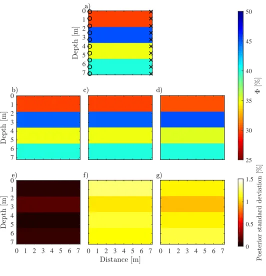
1.1 Examples of conceptual models of subsurface hydrogeological heterogeneity . 6 1.2 The principle of parsimony in the Bayesian approach to model selection . . . . 11 1.3 Simplified representation of a Markov chain . . . 16 2.1 Summary statistics of the posterior porosity distribution for different subsurface

conceptualisation used in the synthetic crosshole-GPR experiment . . . 34 2.2 Mean evidence estimates in log10space and their associated uncertainty for the

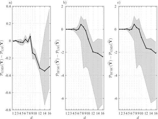
synthetic crosshole-GPR experiment . . . 36 2.3 Difference in the evidence estimates derived from different pairs of methods as

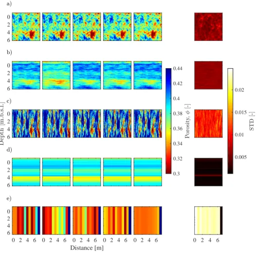
a function of model complexity for the synthetic crosshole-GPR experiment . . 37 2.4 Prior porosity realisations for different conceptual models at the South Oyster

Bacterial Transport site . . . 40 2.5 Posterior porosity realisations and their summary statistics for different

con-ceptual models at the South Oyster Bacterial Transport site . . . 41 2.6 Posterior and prior distributions of the inferred parameters at the South Oyster

Bacterial Transport site . . . 43 2.7 Mean evidence estimates in log10 space and their associated ranges for the

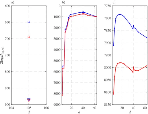
South Oyster Bacterial Transport site . . . 44 2.8 Twice the natural logarithm of the Bayes factors of the competing conceptual

models of the South Oyster Bacterial Transport site . . . 46 3.1 Summary statistics of the posterior porosity distribution using different

ap-proaches to account for the petrophysical uncertainty . . . 61 3.2 Impact of the correlation in the petrophysical uncertainty on the GPR travel

time data residual . . . 62 3.3 Posterior distributions of the inferred porosity mean and variance obtained

from four different assumptions about petrophysical uncertainty . . . 64 3.4 Summary statistics of the posterior porosity distribution using four different

assumptions about petrophysical uncertainty and scatter plots . . . 65 3.5 Mean evidence estimates in log10space and log-likelihood posterior

distribu-tions using four different assumpdistribu-tions about petrophysical uncertainty . . . 67 3.6 Posterior distributions of the inferred porosity mean and variance and of the

inferred geostatistical parameters of the petrophysical uncertainty . . . 69 3.7 Summary statistics of the posterior porosity, petrophysical uncertainty and

velocity models . . . 70 3.8 Posterior realisations of the petrophysical uncertainty . . . 71 3.9 Posterior and prior distributions of the inferred parameters at the South Oyster

Bacterial Transport site . . . 73 3.10 Posterior mean hydraulic conductivity, velocity and petrophysical uncertainty

(13)

3.11 Scatter plots of the mean posterior hydraulic conductivity against GPR velocity estimates assuming three petrophysical relationship . . . 76 3.12 Mean evidence estimates in log10space for three petrophysical relationships . 76

4.1 Model proposal workflow of Graph cuts . . . 89 4.2 Training images used to represent spatial hydraulic conductivity distribution of

the aquifer at the MADE site . . . 91 4.3 Prior hydraulic conductivity realisations generated with Graph Cuts from the

training images proposed at the MADE site . . . 95 4.4 Summary statistics and Gelman-Rubin statistics of the posterior hydraulic

conductivity distribution for each conceptual model at the MADE site . . . 96 4.5 Simulated and measured breakthrough curves from the MADE-5 experiment . 97 4.6 Natural logarithm of the evidence estimates as a function of the number of

MCMC iterations for each conceptual model at the MADE site . . . 98 4.7 Mean of the natural logarithm of likelihoods as a function of power coefficientβ100 4.8 Percentage ratio of the effective number of MCMC samples and discretisation

and sampling errors as functions ofβ . . . 101 4.9 Twice the natural logarithm of the Bayes factors of the competing conceptual

models at the MADE site . . . 102 4.10 Grids used for simulations of the MADE-5 tracer experiment with MODFLOW/

MT3DMS and MaFloT . . . 105 4.11 Hydraulic head profiles arising from 2D and 3D flow simulations and simulated

breakthrough curves with and without model error correction . . . 107 4.12 Simulated and measured breakthrough curves from the MADE-5 experiment in

the monitoring well MLS-1 . . . 108 4.13 Simulated and measured breakthrough curves from the MADE-5 experiment in

the monitoring well MLS-2 . . . 109 A.1 Slice sampling in d dimensions . . . 134 A.2 Illustration of slice sampling . . . 135 A.3 The "true" porosity field used in the synthetic crosshole-GPR experiment . . . 137 A.4 Mean evidence estimates in log10space and their associated uncertainty for the

GMIS, LM and PC estimators . . . 138 A.5 Difference in the evidence estimates derived from different pairs of methods as

function of model dimension . . . 139 A.6 Linear relationship between the number of forward simulations and nl i veand

nr epeat sfor the PC estimator . . . 140

A.7 Difference in the evidence estimates with PC derived from different test cases . 141 A.8 Marginal posterior distributions of the inferred porosity using PC . . . 142 A.9 Mean evidence estimates in log10space for the PC estimator as a function of

nl i veand nr epeat s . . . 143

A.10 Marginal posterior distributions of the inferred model parameters using PC . . 145 A.11 Evidence in log10space derived from the GMIS, LM and PC estimators . . . 146

A.12 Evidence in log10space derived from the GMIS, LM and PC estimators with

different settings . . . 147 A.13 Number of forward simulations for evidence estimation as a function of model

dimension . . . 148 xii

(14)

List of Tables

1.1 Interpretation for the Bayes factor of Kass and Raftery (1995) . . . 10 1.2 Overview of technical details used in the different chapters of the thesis . . . . 21 2.1 Interpretation for the Bayes factor of Kass and Raftery (1995) . . . 29 2.2 Parameters subject to inference of the layered conceptual models at the South

Oyster Bacterial Transport site . . . 38 2.3 Geostatistical parameters of the multi-Gaussian conceptual models at the South

Oyster Bacterial Transport site . . . 39 2.4 Parameters subject to inference of the multi-Gaussian conceptual models used

at the South Oyster Bacterial Transport site . . . 39 2.5 Ranking of the conceptual models at the South Oyster Bacterial Transport site . 45 2.6 Evidence estimates of the conceptual models considered for the synthetic

crosshole-GPR experiment . . . 47 3.1 Standard deviation of the measurements errors, acceptance rate and number

of iterations of the full MCMC and MC-within-MCMC methods . . . 59 3.2 Geostatistical parameters subject to inference of the multi-Gaussian conceptual

models . . . 63 3.3 Bayes factors in log10space of the competing conceptual models . . . 66

3.4 Geostatistical parameters subject to inference of the petrophysical uncertainty 68 3.5 Parameters subject to inference at the South Oyster Bacterial Transport sfite . . 72 4.1 Geostatistical parameters of the multi-Gaussian training image proposed by

Bianchi et al. (2011a) for the MADE site . . . 92 4.2 Hydrogeological facies and their hydraulic conductivity values (Rehfeldt et al.,

1992) observed in the MADE site outcrop . . . 92 4.3 Hydrogeological facies and their hydraulic conductivity values identified from

lithological data from the MADE site (Bianchi and Zheng, 2016) . . . 92 4.4 Summary of MCMC results using the MADE-5 tracer data for three MCMC

chains for each conceptual model . . . 94 4.5 Estimates of the natural logarithm of the evidence with corresponding standard

errors for each conceptual model at the MADE site . . . 99 A.1 nl i veand nr epeat sused in the crosshole-GPR experiment . . . 140

A.2 nr epeat sand nl i veused at at the South Oyster Bacterial Transport site . . . 142

A.3 Setting of the conceptual models at the South Oyster Bacterial Transport site for evidence estimation with PC . . . 144 A.4 Computational time for evidence estimation by GMIS, LM and PC . . . 146

(15)

(16)

Abbreviations

ABC . . . Approximate Bayesian Computation AIC . . . Akaike’s Information Criterion AR . . . Acceptance Rate

BFMC . . . Brute-Force Monte Carlo BIC . . . Bayesian Information Criterion BTC . . . Breakthrough Curve

DIC . . . Deviance Information Criterion EM . . . Expectation-Maximization

GMIS . . . Gaussian Mixture Importance Sampling GPR . . . Ground Penetrating Radar

HM . . . Harmonic Mean

KIC . . . Kashyap’s Information Criterion LM . . . Laplace-Metropolis

MADE . . . MacroDispersion Experiment MAP . . . Maximum A-Posteriori MCMC . . . Markov chain Monte Carlo MLS . . . Multi-Level Sampler MPS . . . Multiple-Point Statistics PC . . . POLYCHORD

pdf . . . posterior density function RMSE . . . Root Mean Square Error SS . . . Stepping-Stone sampling TH . . . Thermodynamic Integration

(17)

(18)

Résumé

Les eaux souterraines sont une ressource fondamentale. Avec la croissance démographique, le changement d’utilisation du sol, les activités économiques, l’urbanisation et le changement climatique, une gestion sûre et durable des ressources en eau souterraine devient de plus en plus cruciale. Cela doit reposer sur une caractérisation précise de l’hétérogénéité des propriétés hydrogéologiques du sous-sol, tâche qui représente toutefois un défi. Première-ment, le sous-sol est caché et la collecte locale de données renseignant sur les propriétés hydrogéologiques est difficile ou trop coûteuse. Deuxièmement, les méthodes géophysiques peuvent permettre une acquisition efficace de telles mesures, elles nécessitent néanmoins la définition des relations pétrophysiques qui sont souvent incertaines et mal connues. Troisiè-mement, la structure géologique des systèmes hébergeant les eaux souterraines est complexe et la définition d’un modèle conceptuel correspondant n’est pas unique. Cela conduit à l’une des sources d’incertitude majeure (et souvent ignorée) dans les études de modélisation, appelée incertitude conceptuelle. La sélection bayésienne de modèles, reposant sur le calcul de l’évidence et sur les facteurs de Bayes, fournit une approche quantitative permettant de comparer et de classer des modèles conceptuels alternatifs et, par conséquent, de prendre en compte l’incertitude conceptuelle. Dans cette thèse, nous étudierons l’utilisation de la sélection bayésienne de modèles en hydrogéophysique et en hydrogéologie en répondant aux questions de recherche suivantes : (1) Les données géophysiques sont-elles appropriées pour guider la sélection de modèles en hydrogéologie ? (2) L’incertitude pétrophysique et sa struc-ture spatiale peuvent-elles être déduites dans des études hydrogéophysiques et quel impact ont-elles sur l’inversion bayésienne et la sélection de modèles ? (3) Comment pouvons-nous réaliser la sélection de modèles lorsque nous ciblons des modèles conceptuels aux structures géologiques réalistes représentés par des images d’entraînement ? Ces objectifs seront traités en utilisant une approche bayésienne complète basée sur les algorithmes de Monte Carlo par chaînes de Markov. Les objectifs de la recherche seront ensuite explorés via des études de cas synthétiques et réels, dans le but de caractériser spatialement les champs de porosité ou de conductivité hydraulique dans les aquifères. Dans notre première étude de sélection bayésienne de modèles en hydrogéophysique, nous concluons que les méthodes géophy-siques peuvent être utiles pour choisir la représentation hydrogéologique du sous-sol qui est la plus étayée par les données disponibles, parmi un ensemble de modèles conceptuels concurrents. Nous proposons une méthode pour prendre en compte et déduire l’incertitude pétrophysique et sa corrélation spatiale. Nous constatons que cette approche conduit à une diminution du biais et à une quantification plus réaliste de l’incertitude et du classement des modèles conceptuels. De plus, nous proposons et appliquons avec succès une nouvelle mé-thodologie pour effectuer la sélection bayésienne de modèles parmi des modèles conceptuels géologiquement réalistes.

Mots clefs : Sélection bayésienne de modèles, hydrogéophysique, évidence, incertitude pétrophysique, incertitude conceptuelle, méthode de Monte Carlo par chaînes de Markov, image d’entraînement

(19)

(20)

Abstract

Groundwater is a fundamental source of drinking water. With population growth, land use changes, economic activities, urbanisation and climate change, a safe and sustainable man-agement of groundwater resources is becoming more and more critical. This needs to rely on an accurate characterisation of the hydrogeological heterogeneity in the subsurface, which is a challenging task. First, the subsurface is hidden from sight and collecting local hydro-geological measurements is difficult or too expensive. Second, geophysical methods can effectively support such measurements but, at the same time, they require the definition of petrophysical relationships that are often uncertain and poorly known. Third, the spatial geo-logical structure of groundwater systems is complex and the definition of the corresponding conceptual model is non-unique. This leads to one of the main (and often ignored) sources of uncertainty in modelling studies, namely conceptual uncertainty. Bayesian model selection relying on evidence computation and Bayes factors provides a quantitative approach for com-paring and ranking alternative conceptual models and, therefore, accounting for conceptual uncertainty. In this thesis, we will investigate the use of Bayesian model selection in hydrogeo-physics and hydrogeology by answering the following research questions: (1) Are geophysical data suitable for guiding model selection in hydrogeology? (2) Can petrophysical uncertainty and its spatial structure be inferred in hydrogeophysical studies and how do they impact Bayesian inversion and model selection? (3) How can we achieve model selection when targeting geologically-realistic hydrogeological conceptual models represented by training images? These objectives will be addressed using a full Bayesian approach based on Markov chain Monte Carlo algorithms. The research goals will be then explored in light of synthetic and field-based case studies with the purpose of characterising spatially-distributed porosity or hydraulic conductivity fields in aquifers. From the first comparative study of Bayesian model selection in hydrogeophysics ever, we conclude that geophysical methods can be valuable in providing guidance about which hydrogeological representation of the subsurface is the most supported by the available data among a set of competing conceptual models. We then propose a method to account for and infer the spatially-correlated uncertainty of petrophysical relationships. We find that this approach leads to less bias, more realistic uncertainty quantification and less overconfident model selection. Moreover, we propose and successfully apply a new methodology for performing Bayesian model selection among geologically-realistic conceptual models represented by training images.

Key words: Bayesian model selection, hydrogeophysics, evidence, petrophysical uncertainty, conceptual uncertainty, Markov chain Monte Carlo, training image

(21)

(22)

Chapter 1 Introduction

Water is essential for human life and nature. Population growth, land use changes, economic activities, urbanisation and climate change contribute to both a decreasing water supply and an increasing water demand (IPCC report by Jiménez Cisneros et al. (2014)). These combining factors are expected to lead to an estimated 40% global water supply shortage by 2030 as reported by the European Commission (2012). Over 95% of the freshwater on the planet, excluding glaciers and ice caps, is found underground and it is a fundamental source of drinking water. Groundwater systems are prone to over-pumping and contamination from agricultural and industrial activities and they are vulnerable to extreme events such as droughts and floods. Over the past 30 years, European water policy has been focused on water resources protection (e.g., quality and sufficient quantity of water). A safe and sustainable management of groundwater resources, as well as reliable assessment of water policies, are becoming more and more critical and they should, in fact, rely on quantitative subsurface modelling studies (Scheidt et al., 2018) that are able to simulate past and present conditions and predict future responses of aquifers to natural and anthropogenic stresses (Maliva, 2016). An aquifer is a geological unit that can store useable amounts of water. The characterisa-tion of the (hydro)geological heterogeneity of an aquifer is fundamental because, at small scales, it is a key controlling factor in flow and transport of contaminants and, at larger scales, it influences the rate, position and magnitude of recharge and discharge areas (Maliva, 2016). The properties, structure and processes taking place in an aquifer are difficult to characterise and not fully understood. Indeed, the subsurface is hidden from sight and collecting local measurements of aquifer hydraulic and transport parameters (e.g., porosity, hydraulic conductivity) is challenging or too expensive. Conventional methods in the field of hydrogeology to gather such measurements consist, for instance, by drilling boreholes for collecting soil samples, logging the penetrated geological formations and/or installing fluid sampling instruments to be used, for example, in pumping and tracer tests (Maliva, 2016). These techniques are invasive, costly and provide only point measurements. Geophysical methods (e.g., ground penetrating radar (GPR), direct current resistivity, electromagnetics, seismics) can effectively support the conventional hydrogeological techniques by collecting complementary information over more extended areas and at a lower cost. This combined approach of using hydrogeological and geophysical data forms since the 1990s the discipline of hydrogeophysics (Rubin and Hubbard, 2005; Vereecken et al., 2006). Hydrogeophysics explores the potential of using geophysical methods to infer, with high resolution, hydrologic parameters and processes and the spatial structure of the subsurface relevant for

(23)

hydrolog-ical investigations. The combination of geophyshydrolog-ical and hydrogeologhydrolog-ical investigations is valuable to improve the mapping and the understanding of subsurface systems.

However, the underlying geology and corresponding hydrogeological parameters will never be exactly known, the processes taking place in subsurface systems will never be fully understood and data are noisy and sparse. Quantifying and acknowledging the degree of "ignorance" is fundamental to reliably manage groundwater systems and to effectively support decision-making (Scheidt et al., 2018).

1.1 Motivation: the Bayesian approach

Studies of subsurface systems are often formulated and solved as inverse problems (Tarantola, 2005). Solving an inverse problem consists in using observed data (measurements collected in the field) and prior information to infer the parameters of interest that describe the system under study and their uncertainties. The scientific approach to tackle such problems involves three steps.

(i) Parameterization: the natural system is conceptualised and parametrised when defining a conceptual model (e.g., simplified representation of the geological structure of an aquifer) and assigning the model parameters values that characterise the system (e.g., hydraulic conductivity values of each lithofacies).

(ii) Forward modelling: simulation of the response of a given conceptual model and values of the model parameters using a forward model. A forward model is often a numerical solver implementing physical laws. For instance, if the data are solute concentrations measured during a tracer experiment, the forward model may consist of a set of equations that are solved on a discretised mesh to simulate flow and transport of a solute in a porous medium. (iii) Inverse modelling: the observed data are compared with the simulated ones and model parameter values are updated in order to infer the actual values of the model parameters. The accuracy of any inference about underlying parameters of interest is affected by sev-eral sources of uncertainty. We can distinguish between the uncertainty in the data, the forward model, the petrophysical relationship and the choice of the conceptual model and its assumptions (i.e., values and parameters associated to it). Indeed, the data are noisy and has a limited spatial coverage. The forward model is a simplified physical description of the system and capture only the main processes of the system that are relevant to the study at hand. Geophysical methods are directly sensitive to physical properties of the subsur-face and petrophysical (also called rock physics) relationships need to be defined to link these properties to the hydrogeological parameters and state variables of interest (Binley et al., 2010). One challenge in hydrogeophysics is that the petrophysical relationships in shallow subsurfaces are often non-stationary, non-unique and poorly understood (Rubin and Hubbard, 2005; Linde et al., 2006b), thereby, affecting the predictive power of the inferred parameters of interest. The identification and conceptualisation of the geological structure of groundwater systems are challenging due to their high heterogeneity and spatial variability.

(24)

The definition of a conceptual model for representing a subsurface system is non-unique (Backus and Gilbert, 1967) and it is one of the main sources of uncertainty in modelling studies (Refsgaard et al., 2006; Bond et al., 2007; Rojas et al., 2008; Pirot et al., 2015; Scheidt et al., 2018); it is often referred to as conceptual uncertainty. The predominant practice in most hydrogeophysical and hydrogeological studies is to estimate the parameters of interest under the assumption of one single (often rather simple) representation of the subsurface and to ignore the uncertainty associated with this choice. Testing alternative conceptual models should be promoted to account for conceptual uncertainty (Refsgaard and Henriksen, 2004; Linde, 2014; Linde et al., 2015b; Nilsson et al., 2006; Refsgaard et al., 2012).

The Bayesian approach is a powerful tool to solve inverse problems and to account for differ-ent sources of uncertainty that affect natural system investigations. The main advantages and limitations of the Bayesian approach are listed below.

Advantages

Uncertainty quantification. The Bayesian approach provides a general and flexible proba-bilistic framework for solving inverse problems (Bayesian inference, Section 1.3.1) that fully quantifies uncertainty. The Bayesian approach allows to simultaneously account for different sources of uncertainty such as those mentioned above.

Clarity. As opposed to a "black box", the Bayesian approach requires that each source of uncertainty is explicitly described and that each step in the inverse problem solution is clearly stated.

Easy interpretation. The uncertainty is quantified in terms of a probability distribution that represents the degree of belief about an unknown parameter of interest. This Bayesian interpretation of probability is more straightforward than the classical (frequentist) point of view (Gelman et al., 2013). Indeed, the uncertainty in classical statistics is expressed in terms of confidence intervals that quantify the probability of a certain parameter value in terms of the fraction of times that value occurred after an infinitely repeated number of inferences. Conceptual uncertainty. The Bayesian approach enables inclusion of conceptual uncertainty. Bayesian model selection (Section 1.3) addresses this type of uncertainty using results from Bayesian inference and the computation of Bayes Factors to answer questions as: Which model among a set of competing conceptual models is most supported by the available data? How well does it perform relative to the other conceptual models in the set?.

Definition of a prior. The Bayesian approach requires an explicit description of prior knowl-edge. This stimulates scientists to think, discuss and delve deeper into this aspect, thereby, contributing to a better understanding of the system at hand. For instance, in subsurface modelling, significant effort has been dedicated in recent years to build more geologically-realistic priors using, for example, multiple-point statistics (MPS). Moreover, describing properly the prior knowledge about a system is a process that may involve different experts and stakeholders, thereby, possibly increasing the confidence in the decision-making process. Limitations

Definition of a prior. There is ongoing research and discussions on how to properly describe the prior knowledge and how the choice of the prior impacts the inference and model

(25)

selec-tion results. The definiselec-tion of a prior is problem specific, subjective, non-trivial and general guidelines on how to choose it does not exist when dealing with spatial hydrogeological property fields. In subsurface system studies, this issue becomes acute when no or only little prior information is available and the scientist is often pushed to choose possibly inadequate prior descriptions, such as, uniform and multi-Gaussian distributions (Scheidt et al., 2018; de Pasquale and Linde, 2017).

Computationally intensive. The Bayesian approach is known to be computationally demand-ing, especially when using large datasets, complex models and many parameters that are to be estimated. The need for integrating competences and increasing collaboration between computational and statistical science in this domain has been identified by the International Society for Bayesian Analysis (Jordan, 2011).

Note that the definition of a prior in Bayesian approaches is controversial and it can been seen both as an advantage and a limitation.

1.2 Conceptual models

A conceptual model is a simplified representation of a real system that is built in order to achieve an improved understanding of that reality and to meet the goals of the modelling study at hand. Conceptual models are built based on the prior knowledge that is avail-able about the system using equations, assumptions, governing relationships and spatial parametrisation in order to make interpretations about the system. "The conceptual model in other words constitutes the scientific hypothesis or theory that we assume for our particular modelling study" (Refsgaard and Henriksen, 2004).

In the field of subsurface systems and in this thesis, a conceptual model is a geological interpretation of the subsurface through the definition of (i) the spatial discretisation and parameterisation of the (hydro)geological heterogeneity, (ii) the prior probability density functions (pdf ) that represent all the possible values that each model parameter can take. The model parameters can be assumed to be known or unknown (inferred from the data). If they are unknown, the most probable values and the associated uncertainties given the data are derived by Bayesian inference (Section 1.3.1). In the field of hydrogeophysics, a conceptual model can also include the definition of a petrophysical model and the prior pdf of their parameters if they need to be inferred. Appropriate conceptual models of (hydro)geological heterogeneity in the subsurface are crucial for a reliable and accurate groundwater modelling (Maliva, 2016).

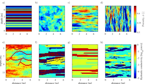
In this thesis, the subsurface heterogeneity is spatially discretised on regular grids. The choice of the grid cell size is driven, for example, by the scale at which we are interested to investi-gate the system heterogeneity, the purpose of the study and computational limitations. The spatial parameterisation of the subsurface heterogeneity is here carried out using a zonation approach, a variogram-based (or two-point) geostatistical approach and a MPS approach. In the zonation approach, the subsurface is subdivided into zones within which the value of the parameter of interest is assumed constant because its variation is negligibly small compared

(26)

to the variations between different zones. The zonation approach is adequate for represent-ing sharp discontinuities in the subsurface geological structure. However, poorly defined locations of the boundaries may lead to biased model parameter estimation (Vanrolleghem, 2010; Linde et al., 2006b). A very simple example of a conceptual model parametrised with the zonation approach is a horizontally layered model (Figure 1.1a ).

The variogram-based geostatistical approach describes the spatial distribution of the pa-rameters of interest as a random field with a correlation structure defined by means and covariances that convey information on the variance and the integral scales of spatial param-eter correlation in different directions (i.e., anisotropy). A classical example of conceptual models built from two-point geostatistics are the multi-Gaussian fields in Figure 1.1b-d. This type of conceptualisation is widely used. However, it is well recognised that they may be simplistic and inadequate to capture the complexity of the subsurface geological structure and, thus, to properly reproduce and predict flow and transport processes in subsurface systems (Gómez-Hernández and Wen, 1998; Journel and Zhang, 2006; Kerrou et al., 2008). Training images offer a means to conceptualise the prior geological knowledge of the system under study and MPS allows to effectively reproduce the complex geological patterns (e.g., curvilinear features) found in the training image (Guardiano and Srivastava, 1993; Strebelle, 2002; Hu and Chugunova, 2008; Mariethoz and Caers, 2014). The first simulation algorithm based on training images and MPS is SNESIM (Strebelle, 2002) that is limited to categorical fields. Efficient and computationally fast simulation algorithms that are able to sample from both categorical and continuous images are, for example, the direct sampling (Mariethoz et al., 2010b) and the recent graph cuts (Zahner et al., 2016) methods. Examples of conceptual models built using graph cuts are shown in Figure 1.1e-h. The prior geological understand-ing is informed by expert knowledge, outcrops and geophysical and borehole data. These informations are then used to create a training image from sketches drawn by hand, digi-talised outcrops, process-imitating, structure-imitating or descriptive simulation methods (Koltermann and Gorelick, 1996; De Marsily et al., 2005).

Conceptual models built with zonation or variogram-based geostatistics imply explicit for-mulas for the prior pdfs (e.g., parametric priors such as Gaussian or exponential functions) of the model parameters. On the other hand, the conceptual models obtained from training images circumvent the definition of parametric priors by using a pseudo-random process (e.g., sequential geostatistical resampling) that produces samples according to the prior distri-bution (Mosegaard and Tarantola, 1995). From this prospective, the prior pdf is represented by a series of simulation steps rather than an explicit formula (Ruggeri et al., 2015) and a specific acceptance criterion in the Markov chain Monte Carlo (MCMC) algorithm is needed in these cases (Section 1.5). For a criticism of this type of approach, the reader is referred to Emery and Lantuéjoul (2014), in which it is suggested that the training image must be of infinite extent to enable a complete uncertainty quantification.

(27)

0 2 4 6 0 2 4 6 depth [m] 0 2 4 6 0 2 4 6 0 2 4 6 0.3 0.35 0.4 P o ro si ty , ? [-] 0 2 4 6 distance [m] 5 7 9 11 depth [m] 0 2 4 6 distance [m] -5 -4 -3 -2 -1 0

Hydraulic conductivity [log

10 (cm/s)] 0 2 4 6 distance [m] 0 2 4 6 distance [m] a) b) c) d) e) f) g) h)

Figure 1.1 – Examples of conceptual models of subsurface (hydro)geological heterogene-ity parameterised with the (a) zonation, (b-d) variogram-based and (e-h) multiple-point geostatistics approaches. The different spatial parameterisations consist of (a) horizontal layers, (b) multi-Gaussian with isotropy, (c) multi-Gaussian with horizontal anisotropy, (d) Gaussian with vertical anisotropy and (e) conductive channels overlapped on a multi-Gaussian field (i.e., combination of continuous and categorical fields) and (f-h) categorical fields (i.e., each facies has a specific value of the hydrogeological property).

1.3 Bayesian model selection

Suppose that an aquifer needs to be characterised in order to perform groundwater model predictions. As previously explained (Section 1.1), direct investigations of the subsurface is challenging, the geological structure is heterogeneous and it has high spatial variability. Several experts, such as geologists and hydrogeologists, can be consulted and asked to pro-vide their insights about the expected aquifer structure based on their experience (prior knowledge). In this process, we might come up with several plausible conceptualisations of the aquifer (hydro)geological structure (e.g., layered, multi-Gaussian, outcrop-based) that span a wide range of groundwater predictions. In many real applications, this conceptual uncertainty is a dominant source of uncertainty and ignoring it may imply a drastic underes-timation of uncertainty on model predictions (Refsgaard et al., 2006; Bond et al., 2007; Rojas et al., 2008; Pirot et al., 2015; Scheidt et al., 2018). How can we deal with such conceptual uncertainty? Bayesian model selection based on Bayes factors (Jeffreys, 1935, 1939; Kass and Raftery, 1995) provides a quantitative approach for comparing and ranking alternative hypotheses relative to each other (probability of one hypothesis to another) in the light of the observed data. Note that the term hypothesis and conceptual model (as defined in Section 1.2) are here used interchangeably.

(28)

This approach of quantifying and improving the state of knowledge about reality by testing and comparing different perceptions of that reality based on the information at hand (data) is fully in line with the concept of falsificationism introduced in Popper’s scientific philosophy (Popper, 2005). All conceptual models are wrong (Box, 1979) and they are not verifiable in the sense that the true conceptual model is never possible to be proven (Konikow and Bredehoeft, 1992; Oreskes et al., 1994). On the other hand, a hypothesis can be corroborated (confirmed) or falsified (refuted) depending on wether or not it is in agreement with the current scientific knowledge (Popper, 2005). If a hypothesis predicts the observed data much more poorly than the other hypothesis, then it is falsified, otherwise, it is retained and tested against new data and hypotheses. This is one view of how science progresses.

Some important aspects should be kept in mind when comparing different conceptual models.

Purpose. The formulation of the research question is the crucial starting point. It should address the final practical purpose or effectively inform the decision makers and it should drive hard thinking about prior knowledge, conceptual model-building and data collection. "A good answer to a poor question [...] is little better than a poor answer to a poor question" (Burnham and Anderson, 2003). Most of the real investigations have an inferential purpose, that is, obtaining the most reliable inferences about the quantities of interest. In these cases, a set of carefully defined conceptual models may be used. On the other hand, if very little prior knowledge (e.g., geological structure, model parameters, governing equations) is available for the system under study, the comparison of alternative conceptual models may be used for exploratory purposes (Burnham and Anderson, 2003) and for guiding the conceptual model-building process based on falsifications. In such a case, the conceptual models should differ as much as possible from each other. For both exploratory and inferential purposes, the set of competing conceptual models should be ideally as large as possible (while staying within the limits of computational constraints).

Importance of data. Data should be of high quality and they should carry information that is relevant specifically to the practical purposes at hand and to the process of decision-making. Therefore, conceptual model selection is useful only if they are compared using such informative data sets. Scheidt et al. (2018) stress the need for more data of higher quality in groundwater management.

Consistency. If enough data are available and if the true conceptual model is part of the set of the competing conceptual models, then Bayesian model selection guarantees the selection of the true model (Berger et al., 2001).

Interpretation of the "best" conceptual model in the set. The conceptual model that performs the best in the set does not mean that it is the one that best represent the full reality; it just suggests that it is the hypothesis in the set that is the most supported by the information in the data (Refsgaard and Henriksen, 2004). Moreover, since the Bayesian approach to model selection naturally honour the principle of parsimony (Section 1.3.2), the "best" model will not be too simple (underfitting) and not too complex (overfitting) and, consequently, estimates and predictions based on this model will not be too overly optimistic (Berger et al., 2001).

(29)

As shown in the following sections, Bayesian model selection based on Bayes factors consists in applying Bayesian inference at two different levels: at the level of the model parameters and at the level of the conceptual model.

1.3.1 Bayesian inference

Bayesian inference is the process of drawing conclusions from data in terms of probability statements about quantities of interest that are not directly observed. This is accomplished by Bayes’ theorem, a learning rule that expresses how prior knowledge about the system under study is updated by a data-dependent term, called the likelihood function, resulting in a posterior pdf that depends both on the prior state of knowledge as well as the data.

Assume that we want to apply Bayesian model selection on a set of m conceptual models,η = {η1, . . . ,ηm} and that each modelηk, with k = 1,...,m, is described by a vector of parameters

θk. At the first level of inference, we infer what the model parameters,θk, of the conceptual

modelηk might be, given n data,Y = {e y_e₁, . . . ,y_e_n}. Applying Bayes’ theorem, we obtain the posterior pdf, p(θ_k|eY,ηk), of the parameters of interestθkas:

p(θk|eY,ηk) =

p(θk|ηk)p(eY|θk,ηk)

p(Y|ηe k)

. (1.1)

The prior pdf, p(θk|ηk), quantifies probabilistically the initial state of knowledge about what

values the model parameters might take before considering the observed data. The likelihood function, L(θk,ηk|eY) ≡ p(eY|θk,ηk), quantifies the plausibility of the model parameters given

the data. Bayesian inference can be performed with any type of likelihood function. However, a Gaussian likelihood function is often used (out of convenience) by assuming uncorrelated and normally distributed data errors with constant standard deviation,σ_Y_e,

L(θk,ηk|eY) = ³q 2πσ2 e Y ´−n exp " −1 2 n X h=1 µF h(θk) −yeh σeY ¶2# . (1.2)

The larger the likelihood the better the forward model,F (θk), predicts the observed data,Y.e The evidence, p(eY|ηk), also called marginal likelihood, evaluates the support provided by the

observed data to the conceptual model,ηk. The evidence is the normalising constant in Bayes’

theorem and, in the case of discreteθk, is defined as p(eY|ηk) =Pθkp(θk|ηk)L(θk,ηk|eY) where

the sum is over all possible values ofθk. However, in most applications,θk is continuous

and, therefore, the evidence is defined as the (multidimensional) integral of the likelihood function over the prior distribution,

p(Y|ηe _k) = Z

p(θk|ηk)L(θk,ηk|eY)dθk. (1.3)

In other words, we can define the evidence as the average (integral) over the parameter space of the likelihood function weighted by the prior pdf. In the first level of inference that focuses on parameter values, the posterior pdf of the model parameters of each conceptual model are inferred and the evidence is neglected because it is solely a normalising constant.

(30)

At the second level of inference, the Bayes’ theorem is applied a second time in order to infer which conceptual model in the set is most plausible given the data. We obtain the posterior probability of the conceptual modelηkas:

p(ηk|eY) =

p(η_k)p(eY|ηk)

Pm

i =1p(ηi)p(eY|ηi)

. (1.4)

The prior probability, p(ηk), of the conceptual modelηkquantifies the prior plausibility that

we assign toηkbefore considering the data. However, specifying the prior probability for

each conceptual model is often not necessary and we assume here that all the competing conceptual models in the set have the same prior probability. This implies that the con-ceptual model ranking is based merely on the evidence estimates. The denominator is the normalising factor of Equation 1.4 and the sum is over all the competing conceptual models in the set,η. It is clear from Equation 1.4 that the evidence is how the observed data update our prior beliefs about a conceptual model.

1.3.2 Bayes Factors and Evidence

The usefulness of a conceptual model to predict data relative to other hypotheses is assessed by Bayes factors (Jeffreys, 1935, 1939; Kass and Raftery, 1995; Morey et al., 2016). If we want to compare two conceptual models of the set,η1andη2, the Bayes’ theorem in Equation 1.4 can

be rewritten in terms of posterior and prior odds ofη1compared toη2:

p(η1|eY)

p(η2|eY)

=p(η1)p(eY|η1) p(η2)p(eY|η2)

. (1.5)

The posterior odds, p(η1|eY)±p(η2|eY) , is the ratio of the posterior probability ofη1andη2

and it quantifies the degree of belief in favour ofη1overη2after observing the data. The

prior odds, p(η1)±p(η2) , is the ratio of the prior probability ofη1andη2and it quantifies

the degree of belief a-priori (before considering the data) in favour ofη1overη2. We are

interested in comparing the performance ofη1againstη2and this information is carried

by the ratio of the evidence of the two competing model (last ratio in Equation 1.5) and it is termed the Bayes factor. The Bayes factor of conceptual modelη1with respect to conceptual

modelη2is defined as the ratio between the posterior and prior odds ofη1compared toη2:

B(η1,η2)= p(η1|eY) p(η2|eY) Á p(η1) p(η2) = p(eY|η₁) p(eY|η₂) , (1.6)

and it expresses how well the observed data were predicted byη1compared toη2.

Jeffreys (1939) and Kass and Raftery (1995) proposed a scale to interpret the Bayes factor (Table 1.1). If Bayes factors, B(η1,ηi), ofη1compared to each competing conceptual model,ηi,

are all > 150, we may selectη1as the best conceptual model in the set; otherwise, if all the

B(η1,ηi)are < 1, we may discardη1from the set. The scale proposed by Jeffreys (1939) and Kass

(31)

may depend on the context and on the judgement of the modeller based on the practical purposes addressed.

Table 1.1 – Interpretation of Kass and Raftery (1995) (slightly different from the original interpretation of Jeffreys (1939)) for the Bayes factor of two conceptual modelsη1andη2.

2 log B(η1,η2) B(η1,η2) Evidence forη1

< 0 < 1 negative (supportsη2)

0 to 2 1 to 3 barely worth mentioning 2 to 6 3 to 20 positive

6 to 10 20 to 150 strong > 10 > 150 very strong

The evidence is the cornerstone of Bayesian model comparison, model ranking, model selection and model averaging. Bayesian model ranking consists in listing the conceptual models of the set from the best one to the worst one according to the decreasing value of the evidence. Bayesian model selection chooses one single (the "best") model from the set that is the one with the highest evidence and uses that conceptual model for inferring the parameter of interest. Bayesian model selection may be justified when Bayes factors in favour of the best conceptual model compared to the other conceptual models in the set are all larger than 150 (Table 1.1). If this is not the case and the evidence values are within two orders of magnitude, then Bayesian model averaging is preferred. Bayesian model averaging (Hoeting et al., 1999) retains all the conceptual models and derives a composite estimation of a quantity of interest, φ, as: p(ϕ|Y) =e m X k=1 p(ϕ|eY,η_k)p(η_k|eY), (1.7)

that is, the average of the posterior probability ofϕ under each of the conceptual models con-sidered, p(θ|eY,ηk), weighted by the posterior probability of each conceptual model, p(ηk|eY)

(Equation 1.4). Bayesian model averaging provides a rigorous assessment of conceptual uncertainty. However, keeping all the conceptual models may not be practical for communi-cation or descriptive purposes (Berger et al., 2001) and, in these cases, selecting the "best" conceptual model of the set may be useful (Clyde and George, 2004).

A powerful property of the evidence is that it intrinsically honours the Occam’s razor principle (Jefferys and Berger, 1992; MacKay, 2003). The Occam’s razor (Thorburn, 1918) refers to what William of Occam suggested in the fourteenth century, "shave away all that is unnecessary", that is the principle of parsimony. When comparing and ranking alternative hypotheses, it is advisable to honour the concept of parsimony, which can be seen as a trade-off between model complexity and goodness of fit. For instance, if two (or more) conceptual models, η1andη2, fit (almost) equally well the observed data,Y, then the simplest one, saye η1, is preferred over the more complex one, η2, thereby, avoiding the well known problem of

overfitting. The complexity of a conceptual model is not easily definable (van der Linde, 2012; Guthke, 2017; Höge et al., 2018), however, for the sake of simplicity, we may refer to it as the

(32)

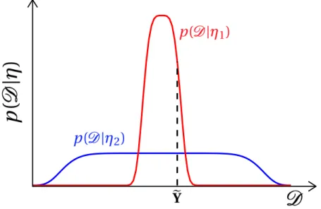
Figure 1.2 – The principle of parsimony in Bayesian model selection. The evidence is here interpreted as the normalised probability distribution, p(D|η), on the space of all possible data sets of fixed size n,D. A more simple conceptual model, η1, spreads the probability

distribution, p(D|η1) (red line), over a smaller range of data sets than a more complex model,

η2, (blue line). Given the observed data set,Y (dotted black line), then it is clear that thee simpler modelη1receives a higher evidence thanη2provided that the two conceptual models

fit (almost) equally wellY and they have equal prior probability. (Figure inspired by the figurese from MacKay (2003); Ghahramani (2013).

number of degrees of freedom (i.e., number of independent model parameters). A more complex conceptual model has more adjustable parameters that allows for a larger range of predictions; vice-versa, simpler models generate a more narrow range of predictions. As a consequence, ifη1andη2fit (almost) equally well the observed data and they have equal

prior probability, then the more complex model,η2, will not predict the observed data set as

strongly asη1, andη1will be favoured (higher evidence) overη2(Figure 1.2). One challenge

in using the evidence for Bayesian model selection is that its computation is difficult and expensive. In most applications of interest, the parameter space is rather high-dimensional and the computation of the integral that defines the evidence (Equation 1.3) has not an analytical solution. Different methods exist to estimate the evidence and we detail some of them in the next section.

1.3.3 Evidence computation

Model selection can either be performed based on analytical expressions based on strong mathematical approximations or numerical estimations of the evidence. The most common approximations are: Akaike’s information criterion (AIC) (Akaike, 1973), deviance information criterion (DIC) (Spiegelhalter et al., 2002; Steininger et al., 2014), Bayesian information criterion (BIC) (Schwarz et al., 1978), Kashyap’s information criterion (KIC) (Kashyap, 1982) and Laplace-Metropolis method (LM) (Lewis and Raftery, 1997) that is closely related to KIC (i.e., KIC=-2logLM). All these mathematical approximations are easy to implement and

(33)

fast to compute, but when the forward model is non-linear and the conceptual models are described by many parameters, most of them (AIC, DIC, BIC) provide poor and inconsistent results (e.g., Lu et al. (2011); Schöniger et al. (2014); Pooley and Marion (2018)).

The LM method evaluated at the maximum a-posteriori (MAP) point is the one that performs the best among the mathematical approximations listed above, (Schöniger et al., 2014). The LM method estimates the evidence by approximating the integrand in Equation 1.3 with a quadratic Taylor series expansion around the MAP estimate,θ∗:

pLM(eY|η) ≈ (2π)d /2|H(θ∗)|1/2p(θ∗|η)L(θ∗,η|Y),e (1.8) where d is the number of parameters in the conceptual modelη and |H(θ∗_{)| is the}

determi-nant of minus the inverse Hessian matrix evaluated atθ∗. The LM is computationally fast but it is built on the strong assumption that the posterior distribution of each parameter of interest is well approximated by a Gaussian distribution that peaks on the corresponding MAP estimate. This underlying assumption should be kept in mind when interpreting the results provided by the LM method.

An alternative to the mathematical approximation of the evidence is to use numerical evalua-tions such as the Brute-force Monte Carlo sampling (BFMC) (Hammersley and Handscomb, 1964), Harmonic mean estimator (HM) (Newton and Raftery, 1994), importance sampling (Hammersley and Handscomb, 1964), thermodynamic integration (TH) (also called path sampling) (Gelman and Meng, 1998; Friel and Pettitt, 2008), stepping stone sampling (SS)(Xie et al., 2011) and nested sampling (Skilling, 2004; Skilling et al., 2006).

The BFMC method consists in drawing randomly N samples of the model parameters,θ, from their corresponding prior distributions and, as the sum of the prior probabilities of the samples equals 1 in this case, the integral of Equation 1.3 can be simply approximated by the average of the likelihood of their prior samples:

pBFMC(eY|η) ≈ 1 N N X i =1 L(θi,η|eY). (1.9)

The accuracy of the BFMC method is ensured by the law of large numbers and the central limit theorem. The BFMC method is an accurate estimator if a very large number of samples is considered and if a large fraction of the prior range has a significant likelihood. For most real-world applications, it suffers from the curse of dimensionality meaning that the computational cost prevent the use of an appropriate number of samples, which leads to underestimation of the evidence. The computational requirements of the BFMC method, thereby, becomes rather impractical for parameter-rich models as many millions or even billions of model evaluations are required to average the likelihood surface.

As opposed to the BFMC, the harmonic mean estimator draws samples from the posterior distribution (e.g., through MCMC methods) and approximates the evidence as the harmonic mean of the likelihood of the posterior samples. This estimator has been proven unreliable (e.g., Newton and Raftery (1994); Liu et al. (2016)). In particular, as this estimator relies only on samples from the posterior distribution (area of high likelihoods) it tends to overestimate the evidence.

(34)

Another numerical approach to evidence estimation is importance sampling. The basic idea of importance sampling is to generate samples from an importance distribution instead of drawing them from the prior distributions as done by the BFMC method. The aim of importance sampling is to focus the sampling to the regions of the distribution that are of most "importance". The resulting bias in the sampling is corrected by attributing a weight to each sample. However, the choice of the importance distribution is not straightforward and it influences the efficiency and robustness of the evidence estimates (Perrakis et al., 2014). Gaussian mixture importance sampling (GMIS) (Volpi et al., 2017) uses as importance distribution an optimal mixture of normal distributions that fit the posterior distribution. The evidence is estimated as a weighted average based on N samples drawn from this importance distribution: pGMIS(eY|η) ≈ 1 N N X r =1 p(θimp_r |η)L(θimp_r ,η|Y)e q(θimp_r ) , (1.10)

where q(θimp_r ) are the importance probability pdf. The GMIS method addresses the problem concerning the choice of an appropriate importance distribution in importance sampling at the expense of an increased computational time. The GMIS works well even in presence of complex multimodal distributions.

A recent approach to evidence estimation that is not based on MCMC algorithms is nested sampling that considers p(θ)dθin Equation 1.3 as equal to the element of prior mass, d X . In this method, a transformation is made fromθto the prior mass X , thereby, reducing Equation 1.3 into a one-dimensional integral over unit range in the likelihood space:

p(Y|η) =e Z 1

0

L(X )d X . (1.11)

The estimation procedure consists in drawing i = 1,..., N samples from the prior distribution under the constraint of a lower bound of the log-likelihood function that increases with time. The one-dimensional integral in Equation 1.11 is then approximated by the weighted mean wiL(Xi) where the weights are defined as wi= Xi− Xi +1. Nested sampling is well suited for

high-dimensional parameter spaces and complex multimodal distributions. However, the exploration of the parameter space based on the likelihood constraint imposed by nested sampling is less efficient than MCMC methods based on the Metropolis-Hastings rule (Section 1.5, Equation 1.20).

Recent studies in hydrology suggest that nested sampling is less accurate and stable than thermodynamic integration (Liu et al., 2016; Zeng et al., 2018). Thermodynamic integration (path sampling) and stepping-stone sampling are based on sampling from a sequence of so-called power posterior distributions, p_β(θ|eY), that create a path in the probability density space connecting the prior to the posterior distribution:

p_β(θ|eY) ∝ p(θ)L(θ|eY)β. (1.12)

The power coefficient,β, varies between 0 and 1. For β=0, the prior distribution is sampled and forβ=1, the posterior distribution is sampled. The normalising constant of Equation 1.12

(35)

is:

p(Y|η,β) =e Z

p(θ)L(θ|eY)βdθ. (1.13)

Assuming a proper prior, Equation 1.13 evaluated atβ=0 is the integral of the prior distribu-tion and it is equal to 1. Equadistribu-tion 1.13 evaluated atβ=1 correspond to the evidence. As a consequence, the thermodynamic integration approach estimates the log-evidence as the integral of the expectations of the log-likelihoods over the interval [0,1] with respect toβ:

log p(eY|η) = p(Y|η,β = 1)e p(Y|η,β = 0)e

= Z 1

0

E_θ_|e_Y,_β£logL(θ|eY,η)¤dβ. (1.14) The one-dimensional integral in Equation 1.14 is then approximated by quadature rule (e.g., composite trapezoidal rule). Stepping-stone sampling is based on a different idea, that is, using importance sampling to acurately approximate the ratio in Equation 1.14. In this context the evidence is estimated as:

p(Y|η) =e K Y k=2 1 N N X j =1 L(θ_k−1,j|eY)(βk−βk−1)_, _(1.15)

where K is the number of the power coefficientsβ. The evidence estimators based on power posteriors are quite easy to implement. However, their accuracy is strongly influenced by the discretisation scheme used for theβ values. The general idea is to place most of them close to zero where the log-likelihood increases the most.

1.4 Petrophysical models

In hydrogeophysics, the effective use of geophysical data for hydrogeological investigations is strongly linked to the reliability of the underlying relationship between estimated geophysical attributes (e.g., permittivity, electrical conductivity, bulk density) and the hydrogeological properties and states variables of interest (e.g., porosity, hydraulic conductivity, water con-tent). The definition of a proper petrophysical relationship is one of the main challenges in hydrogeophysics (Binley et al., 2015) because they are often non-unique and non-stationary, that is, their parameter values and their analytical form can vary drastically between different types of lithologies (Hubbard and Rubin, 2005). Indeed, petrophysical relationships are often treated as site-specific because they depend on the geological structures of the subsurface and this implies that corresponding parameter values need to be calibrated for each site under study. Many relationships have been explored for hydrogeological studies (Mavko et al., 1998; Lesmes and Friedman, 2005; Pride, 2005). The petrophysical relationships can be physically or empirically-based (Linde et al., 2006b). In this thesis, we link GPR data to porosity and hydraulic conductivity properties using a physically and empirically based petrophysical relationship, respectively. The physically based relationship is built using volume-averaging to link the effective relative permittivities,ε [-], to porosity values, Φ [-],

(36)

and to radar slownesses, s [s/m], (Pride, 1994): (ε = Φm_[_ε

w+ (Φ−m− 1)εs]

ε = s2_c2 (1.16)

whereεw[-] andεs[-] are the relative permittivities of water and mineral grains, respectively;

m [-] is the cementation index and c = 3 · 108[m/s] is the speed of light in vacuum. The

slowness, s, is defined as the inverse of the velocity, v.

Combining the equations in 1.16, the petrophysical relationship reduces to: v =

q

Φ−m_c2_[_ε

w+ (Φ−m− 1)εs]−1 (1.17)

The empirically-based relationships are obtained by fitting polynomial functions. In our case, we test linear and quadratic petrophysical relationships to link the GPR velocities, v [m/s], to the natural logarithm of the hydraulic conductivities,K = log K [log(m/h)]:

v = a0+ a1K (1.18)

v = a0+ a1K + a2K2 (1.19)

where a0, a1and a2are the polynomial coefficients.

The petrophysical model consist in the definition of a functional form for the petrophysical relationship and the parameter values needed to describe such relationship. The petrophysi-cal parameter values (e.g., m andεsin Equation 1.17 and a0, a1and a2in Equations 1.18-1.19)

may be inferred within the Bayesian inversion.

1.5 Markov chain Monte Carlo

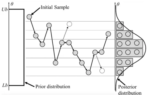
How can we evaluate the posterior distribution of Equation 1.1? In most applications, the posterior distribution cannot be analytically estimated and sampling schemes are needed to numerically approximate it. The MCMC method (Gilks et al., 1995) provides a means to sample high-dimensional and very complicated posterior distributions by combining random sampling (Monte Carlo integration) with a "clever" search within the parameter space by building Markov chains. The resulting Markov chain is a sequence of random variables, {θ0,θ1,θ2, ...}, that are drawn from the model parameter space proportionally to

the posterior distribution such that, at each iteration t , the probability ofθ_{t +1}depends only on the value ofθt. This lack of memory is the Markov property. The posterior distribution

is approximated by the stationary distribution of the Markov chain, that is, the chain will gradually "forget" its initial state and converge to a unique and stationary distribution (i.e., which does not change with t ). This property is ensured by the fulfilment of the ergodicity and