HAL Id: hal-00714717
https://hal.archives-ouvertes.fr/hal-00714717
Submitted on 5 Jul 2012
HAL is a multi-disciplinary open access
archive for the deposit and dissemination of
sci-entific research documents, whether they are
pub-lished or not. The documents may come from
teaching and research institutions in France or
abroad, or from public or private research centers.
L’archive ouverte pluridisciplinaire HAL, est
destinée au dépôt et à la diffusion de documents
scientifiques de niveau recherche, publiés ou non,
émanant des établissements d’enseignement et de
recherche français ou étrangers, des laboratoires
publics ou privés.
Pairwise Markov model applied to unsupervised image
separation
Selwa Rafi, Marc Castella, Wojciech Pieczynski
To cite this version:
Selwa Rafi, Marc Castella, Wojciech Pieczynski. Pairwise Markov model applied to unsupervised
image separation. SPPRA ’11 : The Eighth IASTED International Conference on Signal Processing,
Pattern Recognition, and Applications, Feb 2011, Innsbruck, Austria. �10.2316/P.2011.721-044�.
�hal-00714717�
PAIRWISE MARKOV MODEL APPLIED TO UNSUPERVISED IMAGE
SEPARATION
Selwa Rafi, Marc Castella and Wojciech Pieczynski D´epartement CITI; UMR-CNRS 5157
Institut Telecom; Telecom SudParis 9 rue Charles Fourier 91011 Evry cedex, France
email: [email protected], [email protected], [email protected]
ABSTRACT
The paper deals with blind separation and recovery of a noisy mixture of two binary signals on two sensors. Such a model can be applied in the context of recovery of scanned documents subject to show-through and bleed-through ef-fects. The problem can be considered as a blind source separation one. Due to a complex noise and data structure, it is tackled from the more general approach of Bayesian restoration. The data is assumed to follow a Pairwise Markov Chain model: it generalizes Hidden Markov Chain models but it still allows one to calculate thea posteriori
distributions of the data. The Expectation-Maximization (EM) and Iterative Conditional Estimation (ICE) methods are considered for parameter estimation, yielding an unsu-pervised processing. Finally, simulations show the interest of our approach on simulated and real data.
KEY WORDS
Pairwise Markov Chain, blind source separation, image separation, show-through removal.
1
Introduction
In the last years, Blind Source Separation (BSS) has been an active research area [2]. Independently, Pairwise Markov based models have proved their efficiency for re-covering hidden discrete data, with application to image segmentation [4, 9]. Inspired from the problem formulation of recovery of scanned documents subject to show-through and bleed-through effects [10, 15, 11, 14, 16], we make in this paper a link between the two approaches. We also highlight in this context the interest of Pairwise Markov Chain (PMC) models, which have been recently introduced in [4], and we study the performance of the corresponding methods.
The PMC model is an extension of Hidden Markov Chain (HMC) models [6, 7, 13]. In both models, thea pos-terioriprobability can be calculated, allowing one to imple-ment a Bayesian restoration or segimple-mentation. The interest and the efficiency of the PMC model have been recently illustrated [4] in the case of a scalar observation; in par-ticular, PMC models are able to deal with more complex noise or signal structure.
In this work, for source signals which have a fi-nite number of states, we recast the BSS problem in the more general framework of Bayesian hidden data restora-tion. In our context of vector observed data, we apply a Marginal Posterior Mode (MPM) restoration technique based on a PMC model. This requires first a parameter es-timation which is performed using either the Expectation-Maximization (EM) [9] or Iterative Conditional Estimation (ICE) estimators [4, 3]. In the case of multidimensional data, PMC models are quite involved and we are not aware that it has been considered so far: our work is thus an ex-tension of [4] in the case of a vector observation process. One can expect that PMC models should help dealing with complicated noise structures.
We especially focuse on the separation problem for process vectors whose elements take binary values, black and white images. We also deal with the separation problem of real scanned images. The different models (HMC,PMC) are considered in simulations. We first de-scribe in Section 2 the considered models. Then, estima-tion and restoraestima-tion techniques are explained in Secestima-tion 3. Simulation results are provided in Section 4. Finally, Sec-tion 5 concludes the work
2
Models and notations
2.1 Mixture model and hidden variables
In many applications, the observations can be modeled as a mixture of unknown sources. More specifically, a se-ries of T samples xt, t ∈ {1, . . . , T } of a vector signal
is available, where for any t, xt = (x1t, . . . , x Q t)T is a
Q-dimensional vector. These observations result from a mixture of N unknown source signals. For any sample time t ∈ {1, . . . , T }, the source values are stacked in the vector st = (s1t, . . . , sNt )T. The objective is to
re-store the unknown sources only from the observed values xt, t∈ {1, . . . , T }. In other words, we want to retrieve for any i∈ {1, . . . , N } the signal si
t, t∈ {1, . . . , T }.
In order to propose a solution to the described prob-lem, the process xtshould depend on st. We only assume a
probabilistic dependence and no specific dependence struc-ture. In particular, our method is applicable to the case
where:
xt= M(st) + bt, t∈ {1, . . . , T } (1) whereM(.) denotes an unknown, linear or nonlinear func-tion and btis an additive noise. The structure of btmay
be complicated and in conjunction withM(.) defines the dependency between stand xt. A model such as 1 occurs
when trying to separate two images obtained from a text scanned document subject to ink bleed-through effect.
Finally, we will assume that each component of st
belongs to a finite set and hence the vector stalso belongs
to a finite set denoted byΩ, {ω1, . . . , ωK}. This occurs
when separating only black/white (or gray level) mixtures of images.
In this context, restoring the value of the source vector stis actually equivalent to determining to which class in Ω it belongs. We will hence tackle the problem of source separation similarly to the problem of segmentation. In our work, the parameter models are unknown and need to be estimated. Consequently, the problem is said to be blind or unsupervised.
2.2 Hidden variables models
2.2.1 Temporally iid variables and HMC models We denote by S, (s1, . . . , sT) (resp. X, (x1, . . . , xT))
the set of all samples of the hidden source process (resp. the observation process). The variables (X, S) are gen-erally described by a distribution such that p(X, S) = p(S)p(X | S), where p(.) stands for the probability distri-bution and p(. | .) for the conditional probability. The fol-lowing assumptions are among the most common ones:
A1 p(X | S) =QTt=1p(xt| st);
A2 The vector process st is a stationary Markov
pro-cess, that is: p(S) = p(s1)QT −1t=1 p(st+1| st) and
p(st, st+1) does not depend on t.
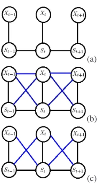
When assumptions A1 and A2 hold, the model is referred to as a Hidden Markov Chain model (see Fig. 1(a)) and the distribution reads: p(S, X) = p(s1) T −1Y t=1 p(st+1| st) T Y t=1 p(xt| st)
One can see that the situation in Equation (1) in Sec-tion 2.1 is also described by the above model as soon as st and bt are mutually independent processes and st is a Markov process : in this case, the conditional density p(xt| st) is given by the density of the noise bt. An even
simpler situation is obtained in the particular case where assumption A2 is strengthened and the vectors stare
tem-porally independent and identically distributed (iid). This case is however very rare in applications and it is generally more realistic to introduce some temporal dependence.
2.2.2 PMC models
It turns out that HMC models present some weaknesses in some situations. For example, S does not necessarily fol-low a Markov process or the additive noise bt in Section
2.1 may depend on the whole process S. In both cases, the HMC model is no longer valid and does not describe cor-rectly the data. In the following we propose to use a PMC model [4] which generalizes the HMC model.
In the PMC model, we consider the process zt ,
(xt, st) and we assume that zt, t∈ {1, . . . , T } is a Markov
Chain (see Fig. 1(b)). This model is strictly more general than HMC [4] because the hidden process st is not
nec-essarily Markov. In a PMC, st is indeed the marginal of
a Markov process. The distribution of Z , (z1, . . . , zT)
is given by p(Z) = p(z1)QT −1t=1 p(zt+1| zt). We will
consider only stationary reversible PMC, in which case p(zt, zt+1) does not depend on t and the distribution of Z
is entirely defined by:
p(zt, zt+1) = p(st, st+1)p(xt, xt+1| st, st+1) (2)
Note that the PMC model becomes a HMC if the following holds [8]:
p(xt, xt+1| st, st+1) = p(xt| st)p(xt+1| st+1)
2.2.3 Gaussian model and PMC with independent noise
Until now, we have not specified the distribution of the observations conditionally on the hidden process. Gaus-sian PMC is a simple possibility, in which the conditional distributions p(xt, xt+1| st, st+1) are Gaussian. Since the
distribution of Z is entirely given by the distributions in (2), it is characterized by K2 probability parameters of p(st, st+1) and K2 joint conditional probability densities
p(xt, xt+1| st, st+1).
As xt is a vector in this paper, the number
of parameters required to characterize each density p(xt, xt+1| st, st+1) may become rapidly large. Since
there are K2 such densities, the problem may become in-tractable. For simplification we consider the specific model of “independent noise PMC” (see Fig.1(c)) which satisfies: p(xt, xt+1| st, st+1) = p(xt| st, st+1)p(xt+1| st, st+1)
(3) As shown in [12], in an “independent noise PMC”, S is not a Markov chain. Hence such a PMC is not a HMC.
We will assume that both p(xt| st, st+1) and
p(xt+1| st, st+1) are Gaussian. When xtis of dimension
Q = 2, p(xt| st, st+1) and p(xt+1| st, st+1) are defined
respectively by the parameters (µi,j1 ,σ1i,j) and (µi,j2 ,σi,j2 ). In the following we consider the bidimensional case (Q= 2).
(a)
(b)
(c)
Figure 1. Graphical dependence scheme of: (a) HMC model, (b) PMC model, (c)Independent noise PMC model.
3
Methods
3.1 Bayesian restoration
3.1.1 Maximum Posterior Mode (MPM)
The hidden vector process S is recovered using the MPM classification method which is based on selecting the class that maximizes the marginal posterior probability. More precisely, the decision rule is:
{bst= ωi} ⇐⇒ {p(st= ωi| X) = max
j p(st= ωj| X)}
3.1.2 Forward-backward procedure
The above restoration method requires to calculate the marginal posterior probability. Let us introduce the follow-ing coefficients: αt(i) = p(st= ωi| x1, ..., xt) βt(i) = p(xt+1, ..., xT| st= ωi, xT) p(xt+1, ..., xT| x1, ..., xT) We have then: p(st= ωi| X) = αt(i)βt(i) (4)
For both HMC and PMC models the coefficient αt(i) and
βt(i) can be calculated exactly with an efficient
forward-backward procedure [4, 5]. No numerical approximation or integration is required to calculate the marginal posterior probability.
3.2 Parameter estimation
As we consider the unsupervised context, we now address the problem of parameter estimation. For each class
transi-tion(ωi, ωj) we calculated 2 mean vectors of size (Q × 1)
and2 covariance matrices of size (Q × Q). 3.2.1 Expectation-Maximization (EM)
A well known parameter estimation method is the itera-tive Expectation-Maximization algorithm, which can also be applied to PMC [9]. After parameter initialization, each loop of the EM algorithm consists of the two following steps:
• ”Expectation” step : we calculate ψt(i, j) = p(st =
ωi, st+1 = ωj| X) the joint probability of being at
time t in the class ωiand at time(t + 1) in the class
ωjknowing the observations.
ψt(i, j) =
αt(i)p(st+1 = ωj, xt+1| st= ωi, xt)βt(i)
P
(ω1,ω2)∈Ω2αt(ω1)p(st+1= ω2, xt+1| st= ω1, xt)βt(ω2)
• ”Maximization” step : we estimate and update the K2probability parameters of p(s
t, st+1) and K2
bi-dimensional parameters defining (3) using ψt(i, j) as
follows: p(st= ωi, st+1= ωj) ← T −11 PT −1t=1 ψt(i, j) b µi,j1 ← PT −1 t=1 ψt(i, j)xt PT −1 t=1 ψt(i, j) b µi,j2 ← PT −1 t=1 ψt(i, j)xt+1 PT −1 t=1 ψt(i, j) b Γi,j1 ← PT −1
t=1 ψt(i,j)(xt−µbi,j1 )(xt−µbi,j1 ) T PT −1 t=1 ψt(i,j) b Γi,j2 ← PT −1
t=1 ψt(i,j)(xt+1−µbi,j2 )(xt+1−µbi,j2 ) T
PT −1 t=1 ψt(i,j)
3.2.2 Iterative Conditional Estimation (ICE)
Another way to estimate the model parameters consist in using the ICE algorithm which has shown a remarkable flexibility [4]. It is based on the conditional expectation of any estimator valid when the complete data Z= (S, X) is available: all parameters are estimated as soon as samples of X according to p(X | S) can be simulated. Concretely after parameter initialization, the ICE algorithm consist in successively sampling X according to p(X | S) and updat-ing the parameters. p(st= ωi, st+1 = ωj) is obtained the
same way as in EM and the other parameters are given by: b µi,j1 ← 1 Card(Ai,j) PT −1 t=1 1Ai,jxt b µi,j2 ← 1 Card(Ai,j) PT −1 t=1 1Ai,jxt+1 b Γi,j1 ← PT −1
t=1 1Ai,j.(xt−bµi,j1 )(xt−bµi,j1 ) T
Card(Ai,j) b
Γi,j2 ← PT −1
t=1 1Ai,j.(xt+1−µbi,j2 )(xt+1−µbi,j2 ) T
Card(Ai,j)
where Ai,jdenotes the set of indices1 ≤ t < T for which (st, st+1) = (ωi, ωj) ∈ Ω2.
4
Simulation Results
Similarly to the previous section, Q = 2 observations are available in our simulations. The vector hidden process st
is also of dimension N= 2 and it consists of two processes si
t, i∈ {1, 2} which are assumed to take binary values ±1.
Equivalently, we consider that st belongs to the setΩ =
{(±1, ±1)} composed of four classes. This experimental setting corresponds to the considered application of bleed-through effect in scanned documents.
4.1 Simulated processes 4.1.1 Data generation
We first tested our method on simulated processes with T=2000 samples. The process stwas either iid distributed
(table 2) or was a Markov chain (table 1, case HMC) with transition parameters: aij = 0.8 0.1 0.05 0.05 0.1 0.8 0.05 0.05 0.1 0.05 0.8 0.05 0.1 0.05 0.05 0.8
The two sources have been mixed linearly with ma-trix M= (0.8 0.7
0.7 0.8) and a noise has been added.The global
model can hence be expressed by the following equation: xt= Mst+ bt (5) The nois btis independent of stand presents either of the
following characteristics:
• iid noise: In this situation, chains are corrupted with an independent noise (with variance equal to0.4), the global model obtained follows HMC model.
• PMC noise: a more complex situation is to consider a noise following a PMC model in which the depen-dency between successive observations conditionally on the successive hidden sources p(xt, xt+1| st, st+1)
is given by a Gaussian distribution defined with2(K2)
variance parameters. 4.1.2 Restoration results
The MPM restoration is completely unsupervised: all pa-rameters are unknown and are estimated by the algorithm (either EM or ICE). The simulations results are collected in the following tables :
Method iid noise (s1, s2) PMC noise (s1, s2) PMC-ICE (12.3, 11.8) (29.6, 31.9) PMC-EM (11.3, 11.7) (29.7, 31.3) HMC (12.2, 11.3) (35.6, 38.2)
Table 1. Misclassification rates for Markov Chains in%
For the first column of the table 1, the data follows the HMC model. We can observe that PMC model has ap-proximatively the same behaviour as HMC model. How-ever, when the data does no longer follow an HMC model (second column), the PMC algorithm consistently performs better than HMC. This proves that PMC model is more gen-eral than the HMC model.
Method iid noise (s1, s2) PMC noise (s1, s2) PMC-ICE (22.7, 22.9) (34.7, 32.4) PMC-EM (20.0, 19.4) (34.6, 32.5) HMC (20, 8, 20.4) (35.5, 36.4)
Table 2. Misclassification rates for iid Chains in %
For the table 2 especially in the second column, the data follows neither HMC model nor the PMC model. The structure of the global process is unknown. The results show that the PMC model is more advantageous than the HMC model.
We deduce from tables 1 and 2 that the PMC model is a generalization of HMC model. The results obtained for PMC with EM and ICE algorithms are comparable. 4.2 Noisy mixture of real images
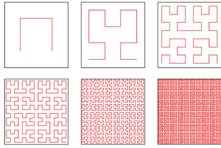
In this section, we present results regarding the application of Gaussian PMC model in image separation. Similarly to [4, 9, 1] we transform the images into chains using the Hilbert-Peano scanning of the image (see Fig.2) .
Figure 2. Hilbert-Peano curves and scannings for images of respective size: 2×2, 4×4, 8×8, 16×16, 32×32, 64×64.
We considered the two black and white images (each color corresponding to+1 or −1) showed in Fig.3. Simi-larly to the previous experiment, they have been mixed ac-cording to (5) with the same matrix M as previously.
We have considered two different noise which are de-scribed in Sections 4.2.1 and 4.2.2 respectively. Images are
Figure 3. Original images (128×128 pixels)
recovered using MPM restoration and the parameters have been estimated with the ICE algorithm.
4.2.1 Mixture of numerical images affected with noise following a PMC model
In this experiment, we take the images in Fig. 3 that we mix with M and we have added a noise following a Gaussian PMC model as in Section 4.1.1. The observations are in Fig. 4.
Figure 4. Mixed images affected with a PMC noise
The MPM restoration with PMC model on Fig.5(b) gives results better than results obtained with HMC on Fig.5(a). It is due to the inability of HMC model to take into account the dependency between noise and sources.
In the following section we consider a correlated noise model which more realistically corresponds to the sit-uation encountered in the show-through and bleed-through effects.
4.2.2 Mixture of numerical images affected with a cor-related noise
In this section, we consider the same mixture as the previ-ous experiment. Each noise component is now correlated and has been generated according to:
b(r) = 1 1 + 4a[ε(r) + a 4 X i=1 ε(ri)]
where r denotes an image pixel, ε(r) is an iid image Gaussian noise, ε(ri) i = 1, . . . 4 are the noise value at
four neighbors of r in the image and a is a given parameter.
17.99% (a) 18.06%
7.32% (b) 8.76%
Figure 5. Separated images and missclassification rate with (a) MPM based on HMC and ICE, (b) MPM based on PMC and ICE. The misclassification rate is given by the percent-age of the restored impercent-age pixels that are different from the original image pixels.
The hidden data has been recovered using MPM method with HMC and PMC model. The results are re-spectively represented in Fig. 7(a) and Fig. 7(b).
The MPM restoration with the PMC algorithm (Fig. 7(b)) is better than the restoration based on HMC al-gorithm (Fig. 7(a)). Like in the case of simulated chains, the algorithm based on PMC shows a better performance in image separation than the method based on HMC model. It is due to its capacity to consider the characteristic of all elements on the mixture and it proves that PMC are more general than HMC.
Figure 6. Mixed images affected with a correlated noise, a = 0.7
4.3 Real scanned images with show-through effect In this section we consider the problem of show-through and bleed-through effects in scanned document [10, 15, 11, 14, 16]. In this situation, we propose to apply our algorithm which allows a good separation automatically without any
18.62% (a) 22.75%
7.10% (b) 7.49%
Figure 7. Separated images and missclassification rate with (a) MPM based on HMC and ICE, (b) MPM based on PMC and ICE.
manual intervention. We compare the performance of the PMC algorithm with respect to HMC model. In both algo-rithms (PMC and HMC) the estimation of the parameters is done using ICE. Fig. 8 shows the recto and verso scan of the same real document, the show-through phenomenon is clearly observed. Fig. 9(a) represents the images restored by HMC model, and in Fig. 9(b) the images are obtained by restoration based on the PMC model.
From these figures, we can conclude that the HMC model is not able to separate correctly the handwriting at each side in the document contrary to PMC model which yielding intersting results. Further investigations on how to apply PMC for the bleed-through problem seem promising.
Figure 8. Real scanned document with show-through effect (from://www.site.uottawa.ca/ edubois/documents).
5
Conclusion
In this paper we have presented the application of the re-cent PMC Model to signal and image separation. The main
(a)
(b)
Figure 9. Images separated with (a) MPM based on HMC and ICE, (b) MPM based on PMC and ICE.
contribution was to extend PMC algorithm to multidimen-sional observed data. The PMC model is richer and more general than the classical HMC model and allows one to take into account more complicated noise structures. We have first validated the performance of the proposed al-gorithm in the case of simulated iid sources and Markov chains sources. We have applied our method to image sep-aration for both synthetic and real images. We have used Bayesian restoration techniques in the context of PMC, and then we have illustrated that PMC models are more effi-cient than HMC models. We have shown that using the proposed method, the problem of source separation can be solved even in delicate situations.
References
[1] Btissam Benmiloud and Wojciech Pieczynski. Es-timation des param`etres dans les chaˆınes de markov cach´ees et segmentation d’images. Traitement du sig-nal, 12.
[2] Pierre Comon and Christian Jutten. Handbook of Blind Source Separation, Independent Component Analysis and Applications. 2010.
[3] Jean Pierre Delmas. An equivalence of the EM and ICE algorithm for exponential family. IEEE Trans.Signal Processing, 45:2612–2615, Oct. 1997.
[4] St´ephane Derrode and Wojciech Pieczynski. Sig-nal and image segmentation using pairwise markov.
IEEE Transaction on Signal Processing, 52(9), Sept. 2004.
[5] Pierre A. Devijver. Baum’s forward-backward algo-rithm revisited. Pattern Recognition Letters, 3:369– 373, 1985.
[6] Yariv Ephraim and Neri Merhav. Hidden markov pro-cesses. IEEE Trans. Inform. Theory, 48:1518–1569.
[7] Timo Koski. Hidden markov models for bioinformat-ics. Kluwer Academic Publishers, 2001.
[8] Pierre Lanchantin, J´erˆome Lapuyade-Lahorgue, and Wojciech Pieczynski. Unsupervised segmentation of randomly switching data hidden with non-gaussian correlated noise. Signal Processing, 2(91):163–175.
[9] Pierre Lanchantin and Wojciech Pieczynski. Un-supervised non stationary image segmentation using triplet markov chains. Advanced Concepts for Intelli-gent Vision Systems (ACVIS.04), Sept. 2004.
[10] Farnood Merrikh-Bayat, Massoud Babaie-Zadeh1, and Christian Jutten. A nonlinear source separa-tion solusepara-tion for removing show-through effect in the scanned documents. 16th European Signal Process-ing Conference EUSIPCO.08, Aug. 2008.
[11] Boaz Ophir and David Mallah. Show-through cancel-lation in scanned images using blind source separa-tiob techniques. IEEE Int.Conf. on Image Processing ICIP-07, 3:233–236, 2007.
[12] Wojciech Pieczynski. Multisensor triplet markov chains and theory of evidence. International Journal of Approximate Reasoning, 45(1):1–16, 2007.
[13] Lawrence R. Rabiner. A tutorial on hidden markov models and selected application in speech recogni-tion. Proc.IEEE, 77:257–286, Feb. 1989.
[14] Gaurav Sharma. Cancellation of show-through in du-plex scanning. Proc. IEEE Int. Conf. Image Process-ing, 2:609–612, Sept. 2000.
[15] Anna Tonazzini, Emanuele Salerno, Matteo Mochi, and Luigi Bedini. Bleed-through removal from degraded documents using a colour decorrelation method. Proc. Document Analysis Systems VI: 6th International Workshop, Springer-Verlag GmbH, LNCS, 3163:229–240, 2004.
[16] Christian Wolf. Document ink bleed-through removal with two hidden markov random fields and a single observation field. IEEE Transactions on Pattern Anal-ysis and Machine Intelligence (PAMI), 32(3):431– 447, 2010.