RESEARCH OUTPUTS / RÉSULTATS DE RECHERCHE
Author(s) - Auteur(s) :
Publication date - Date de publication :
Permanent link - Permalien :
Rights / License - Licence de droit d’auteur :
Bibliothèque Universitaire Moretus Plantin
researchportal.unamur.be
University of Namur
Evolution of a population of protocells: Emergence of species
Carletti, Timoteo; Fanelli, Duccio
Published in:Proc. of the 2006 International Symposium on Mathematical and Computational Biology
Publication date: 2007
Document Version
Early version, also known as pre-print
Link to publication
Citation for pulished version (HARVARD):
Carletti, T & Fanelli, D 2007, Evolution of a population of protocells: Emergence of species. in R Mondaini & R Dilão (eds), Proc. of the 2006 International Symposium on Mathematical and Computational Biology: BIOMAT 2006. E-papers editora, Brasil.
General rights
Copyright and moral rights for the publications made accessible in the public portal are retained by the authors and/or other copyright owners and it is a condition of accessing publications that users recognise and abide by the legal requirements associated with these rights. • Users may download and print one copy of any publication from the public portal for the purpose of private study or research. • You may not further distribute the material or use it for any profit-making activity or commercial gain
• You may freely distribute the URL identifying the publication in the public portal ?
Take down policy
If you believe that this document breaches copyright please contact us providing details, and we will remove access to the work immediately and investigate your claim.
EVOLUTION OF A POPULATION OF PROTOCELLS: EMERGENCE OF SPECIES
T. CARLETTI∗†
D´epartement de Math´ematique, FUNDP 8 rempart de la vierge
B5000 Namur, Belgium tel +32 81724903 fax +32 81724914
E-mail: [email protected]
D. FANELLI
Dipartimento di Energetica ”S. Stecco”, University of Florence and INFN via S. Marta 3
50139 Firenze, Italy E-mail: [email protected]
Keywords: Protocell; Chemoton model; Evolution; Speciation; Chaos
The G´anti Chemoton represents a minimalist description of a protocell unit based on three coupled chemical networks, namely a proto–metabolism, a template du-plication and the membrane growth. We here propose an improved version of G´anti’s “unit of life”where the effects of the volume changes, due to the membrane growth, are explicitly taken into account. The model is further completed by pos-tulating a stochastic mutation mechanism that acts on the template duplication. Within this framework we investigate the evolution of a population of protocells and demonstrate that our hypothesis translates into an open–ended Darwinian evolution, under the pressure of the environment. This observation enables us to conclude that the Chemoton is also a ”unit of evolution”: differentiation into species is indeed an emergent property of the model.
1. Introduction
Almost all life forms known today are composed by cells, fundamental con-stituting units which are able to self–replicate and evolve through changes ∗Work partially supported by contract FP6–002035 of the European Integrated Project
in the EU FP6–IST–FET Complex Systems Initiative PACE.
†This author will present the full paper if accepted.
in genetic information, once selection is active, for instance due to the com-petition for resources.
These highly sophisticated devices are the product of about four billion– years evolution, and, in this respect, represents the relic of primordial life bricks, the protocells. It is customarily believed that the latter were most probably exhibiting only few simplified functionalities – nonetheless nec-essary to consider the protocells alive 1,14,18 – that required a primitive
embodiment structure, a protometabolism and a rudimentary genetics, so to guarantee that offspring were “similar”to their parents.
Artificial protocells have not yet been reproduced in laboratory and intense research programsaare being established aiming at developing
ref-erence models9,13 that capture the essence of the first protocells appeared
on earth and enable one to monitor their eventual subsequent evolution. In 1971, G´anti 6,7 proposed a pioneering theory that provides a
mini-malist description of a protocell, termed Chemoton, i.e. a simplified model to describe growing and multiplying microspheres controlled by a template duplication process. The original minimal Chemoton hypothesis6includes
a membrane which protects the inner bulk, while filtering the access of generic high energetic “food”, which is made available in the surround-ing environment. The food is thus metabolized through chemical reactions and transformed into basic chemical constituents that are needed to stim-ulate both template duplication and membrane growth. Finally, in the simplest scheme, the template–polymer is assembled from one specific type of monomer (homopolymer), which acts as an effective carrier of informa-tion: its length determines in fact the division time, a phenotype prop-erty of paramount importance. After such a time, the protocell attains a critical size, above which a division into two perfect halves occurs. It is thus assumed that cell division occurs as a result of a purely physical pro-cess9. Further, we also assume that each daughter cell contains an
identi-cal amount of chemiidenti-cal material, which is equally shared from the mother constituents. Thus, according to the definition proposed in18,1,14,16, the
Chemoton hypothesis defines a unit of life.
In 7 G´anti raised the following natural question: can one assume the Chemoton to represent also a unit of evolution16 ? To provide a definite
answer to the above question, one has to monitor the dynamical evolution of a population of Chemoton, instead of focusing on the single protocell
aFor instance PACE – Programmable Artificial Cell Evolution – an European Integrated
case. Moreover, the influence of the environment on each protocell needs to be properly incorporated into the model.
With respect to the original Chemoton picture, we here develop an improved formulation (see also 2,3): chemical reactions occur in a
vary-ing volume, the latter bevary-ing intrinsically controlled by membrane growth. This volume effect is explicitly accounted for and shown to significantly contribute to the underlying dynamical process. Moreover, the original deterministic model is further modified to accommodate for an effective mutation mechanism: during the template duplication extra monomers are added (removed) according to a pre-assigned probability, to mimic a stochastic source of errors in the duplication process.
Within this novel scenario, the time evolution of a single protocell is monitored as functions of a number of selected variables of key relevance. This knowledge translates into a State Function which unambiguously pre-dicts the ultimate fate of the protocell, once the specifications of the pro-tocell, e.g. the length of the polymer (N ) and its ability to self–replicate (V∗), and the environmental condition, e.g the external available food ( ¯X),
are assigned.
In particular, assuming that the external food is periodically available, each cycle being for instance associated to tides in the pond were the pro-tocells supposedly live, or the metabolic process to be driven by a periodic source of energy, e.g. the light from the sun, then the regular functioning of the model, i.e. periodic growth and division in time of the protocell, relies on the synchronization of the three chemical networks2.
Motivated by this observation, we previosuly2,3assumed that only
pro-tocells with regular behavior give rise to next generation offspring, while non–synchronized protocells will eventually die. Within this approxima-tion, we provided clear evidence that the model exhibits a simple speciation mechanism, which truly appears as an emergent property. We here adopt a definition of species for asexual beings, based on differences between their genomes4,11,8, which in our setting is equivalent to different lengths of the
double–stranded templates.
The validity of our former strategy, “conservative”form an evolutionary point of view (i.e. non–synchronization implies death), is in turn confirmed by the absence of intermittency (data not shown) in the protocell dynamics. In this paper we take one step forward by relaxing the above hypothe-sis: protocells can attain the duplication threshold at different times. The period of the cycle is hence a characteristic associated to each unit.
because of the use of the State Function concept, a technical solution that allows us to simulate the long time evolution of a large family of protocellsb.
Being the protocells subjected to the pressure of the environment, here ex-emplified through the amount of available food, which changes in time and depends self–consistently on the size of the population: the larger the num-ber of protocells, the lower the amount of available food, and vice–versa. This open-ended mechanism reproduced in this context mimics therefore an effective Darwinian evolution.
As we shall see, protocells with different templates can develop from a common ancestor, due to the combined action of two Darwinian forces: the mutation mechanism and the competition for the available food. The occurrence of a speciation mechanism in a Chemoton–like population is here demonstrated with reference to the above, generalized, setting. This result contributes to shed new light into the important issue of protocells evolution and dynamics: The Chemoton hypothesis defines not only a reliable unit of life, but also a unit of evolution, once the protocell shape is taken into account. Observe in fact that this remarkable feature cannot be obtained in the spherical–shaped Chemoton model7,12, when both volume dependence
and stochastic mutation are accounted for.
2. The model
For the sake of completeness, let us start by briefly introducing the original Chemoton model. The interested reader can refer to to 2,6,7 for further details.
G´anti’s Chemoton model is composed by three chemical networks cou-pled together and schematically outlined in Table 1.
The metabolic autocatalytic cycle is decomposed in five elementary steps, each involving one of the chemicals A1, . . . , , A5. Its role is to
trans-form the highly energetic, externally available, “food”, ¯X, into internal ma-terials (i.e. the precursor of membrane molecules, T′, and the monomers
V′) which sustain the growth and self–reproduction processes. The food is
here supposed to be buffered into the surrounding environment and there-fore assumed constant inside the protocell. The metabolism produces also bEach protocell behavior is described by more than one hundred of equations, computing
the State Function once for all, enables to formally assimilate each protocell belonging to the population under scrutiny to a black box, which produces specific output, once selected input values are provided. This reduces considerably the computational costs and allows to significantly enhance the statistics over previous investigations.
some “waste”, ¯Y , which is progressively eliminated so to maintain its level constant inside the membrane. Each reaction is reversible and therefore in-volves direct and inverse rate constants labeled, respectively, kiand ki′. The
latter are set to the values proposed by G´anti in7and reported in Appendix
A.2.
The second subsystem involves the double–stranded template, i.e. the carrier of the information. Since the model deals with homopolymer species, then the information is carried by the length of the double–stranded tem-plate. As a first step, we assume a constant length of the template, identi-fied by a sequence of N of monomers. In the subsequent analysis, we shall instead introduce a mutation mechanism acting on the template, which, in particular, can alter the polymer length. Due to the thermical fluctuations the bonds at the extremities of the doubled stranded template can open, an event that occurs with high probability. Consequently, when a large enough number of free monomers is available in solution ([V′] ≥ V∗, V∗being the
polymerization thresholdc), the duplication reaction initiates and is further sustained (strong replication condition 12). If the polymer has length N ,
after 2N steps these nested reactions will produce a second identical copy of the double–stranded template and, as by product, R molecules which will allow the transformation of T′ into a membrane molecule T .
The last subsystem governs the dynamical expansion of the growing membrane, which defines the container delimiting the portion of volume where all reactions occur. It avoids the dispersion of useful chemicals, allows the entrance of food and expells the waste. Once a membrane molecule is produced from a precursor T′ and a molecule R, via an intermediate state
T∗, it is then incorporated into the membrane, thus contributing to its
growth. The increase of the membrane is proportional to the membrane size and to the concentration of membrane molecules17: dS
dt = k10T S, k10
being a positive proportionality factor.
The three subsystems are hence coupled together and the effective func-tioning of the Chemoton machinery relies on the precise synchronization of the cycles, which should be thefore maintained in time.
We adopt here a deterministic approach to solve the chemical equations. A system of kinetic differential equations is introduced to describe the time evolution of the chemical concentrations. Such a system is reported in
cThis quantity provides an indirect measure of the attitude for polymerization once
monomers have been selected. The lower V∗, the more pronounced the ability of the
Table 2. As usual, upper dot stands for time derivative while, to lighten notations, capital letters refer to the concentrations.
Moreover, we assume that once the membrane size has doubled, with respect to its initial value, the protocell halves into two smaller offspring, due to physical instabilities. This event defines the protocell cycle.
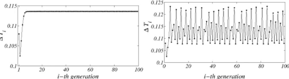
In Fig. 1 two typical behaviors of the division time as function of the generation number are displayed. The simulations refers to one individual protocell. The interested reader can refer to Appendix A.2 for a detailed account on the numerical scheme here adopted. The plot on the left re-ports a periodic, regular, orbit: after a short transient the division time converges to an fixed asymptotic value. This in turn implies that a popula-tion composed by such individuals could be ideally synchronized and share an identical genetic content at the division event. Moreover the population size will increase exponentially opening the way to possible a Darwinian se-lection5,15. The right panel of Fig. 1 shows an irregular orbit: the division
time depends on the generation number. In this case, a virtual family of protocells would be composed by units that divide faster than other, thus possibly resulting in different amount of the inner chemicals, including also the double–stranded template, propagated to the offsprings.
Figure 1. The Division Time. On the left panel we plot the division time as a function of the generation number, for a regular, i.e. periodic, behavior. After a short transient, the division time attains a fixed value: protocells belonging to different generations employ the same amount of time to take the division step to completion. On the right panel an irregular, i.e. non-periodic, behavior. The division time depends on the generation number and it never achieves an asymptotic constant value.
In the original model proposed by G´anti the Chemoton always keeps a spherical shape when growing: this is an important assumption because the behavior of the protocell is determined by the concentrations of the chemicals. Since the volume of the protocell changes in time, one has to properly insert this information into the relevant chemical equations.
Assume the rate of variation (with respect to time) of a given concentration, ci, at fixed volume, to be given by fi(¯c), where ¯c = (c1, . . . , ck). Then
allowing the volume V ol to change, yields: dci dt = fi(¯c) − ci 1 Vol dVol dt , (1)
and each chemical equation in Table 2 has to be modified according to eq. (1).
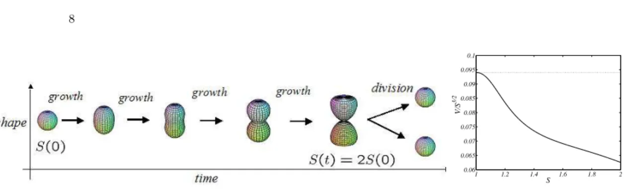
From the chemical equations, one deduces the time evolution of the outer surface: assuming a specific dependence of the volume vs. the sur-face one can eventually monitor the dynamical variation of V ol. We here hypothesize that the protocells pass from an almost spherical shape to a typical hourglass profile close to the duplication event. The existence of an inner pinch is also confirmed by inspection of real cells’ behaviour. The typical evolution of a protocell is schematically depicted in the left panel of Fig. 2. The mathematical details are instead discussed in Appendix A.1.
As already anticipated, the deviations from the original, spherical, pro-file play a central role. For a given surface, in fact, the shape determines the volume enclosed by the membrane and consequently affects the rela-tive concentrations. The sphere maximizes the inner volume which in turn implies that other, more realistic shapes would delimit smaller portions of space, hence resulting in higher concentration. This observation is exempli-fied in the right panel of Fig. 2 where the ratio V (t)/[S(t)]3/2 is displayed
as function of the surface size for the case considered in this study. Observe that, for the case of a sphere such a ratio, is constant and equal to 1/(6√π). Let us observe that already in12, a first attempt has been made to esplicitly
account for volume changes. In that work, however, the authors still assim-ilate the protocell to a sphere, during all stages of its evolution. Following our approach, the protocell shape gradually progresses towards a smooth splitting, that contributes to effectively reduces the functional discontinu-ities observed within the original Chemoton picture12, in conjunction with
a duplication event. (See also Appendix A.1)
To make the model more realistic we further introduce a mutation mech-anism, acting on the double–stranded template. Observe that the genome of each protocell is completely specified through its length, N , and the as-sociated ability to polymerize, V∗. It is thefore quite natural to directly
act on the length of the polymer. A mutation is an error occurring dur-ing the template reproduction: instead of one monomer, two (or more) monomers are added or removed, with a prescribed probability. Alter-natively, we can imagine to introduce a second mutation mechanism: as
1 1.2 1.4 1.6 1.8 2 0.06 0.065 0.07 0.075 0.08 0.085 0.09 0.095 0.1 S V/S 3/2
Figure 2. Behavior of the protocell shape in time. left panel Time snapshots of the protocell evolution. At t = 0 the protocell is assimilated to a sphere whose surface is S(0) = 1. At the division time, the surface has doubled, S(T ) = 2S(0) and the shape resembles a hourglass. right panel The ratio V /S3/2 against the surface size, S. The
black line stand for our model, while the dotted line refers to the case of a sphere. Note that, by assumption, at S = 1 the two curves coincide.
already observed, the polymerization threshold V∗ provides a measure of
the tendency to polymerize. One can therefore assume that the spatial 3D configuration (e.g. right and left helices of ammino–acids) attained by the monomers in the template cooperatively enhances, or viceversa contrast, the polymerization, which practically translate in a modification of the re-lated polymerization threshold. This effect can be mimicked by a second mutation mechanism responsible for altering the initial value of V∗.
The action of our mutation mechanisms is then algorithmically sum-marized as follows: the protocell starts its division cycle with some spec-ification of the double–stranded template, say (N0, V0∗); then, it grows,
produces the needed inner chemicals and duplicates the double–stranded template. Once the membrane size reaches the threshold value, the pro-tocell halves into two offspring, splitting the inner elements and also the polymers, which can in principle be different from the initial ones due to possible mutations occurred during the template duplication. Each daugh-ter is therefore characdaugh-terized by new specifications of the double–stranded template, respectively (N1, V1∗) and (N2, V2∗).
In the following we shall adopt our improved theoretical framework to numerically investigate the time evolution of a family of protocells. 3. Results and Conclusions
Interestingly enough, no complete stochastic simulations of a Chemoton– like model has been attempted so far, except2,3, the reason being ascribed
mainly to the huge computations involved, when tracking the evolution of each single protocell while the population size increases exponentially due
to the combined effect of the duplication and mutation mechanisms. As already mentioned, we overcome these technical difficulties by defining an innovative numerical strategy, briefly recalled below.
The time evolution of a single protocell is monitored as functions of a number of selected variables of key relevance, e.g. the amount of food initially available, the template length and its polymerization threshold at start. This information is used to build up a State Function which enables one to predicts the ultimate fate of the protocell under scrutiny once the ini-tial conditions are specified and without resorting to additional numerical integration. More precisely, for each choice of parameters values (N, V∗),
defined over a large grid, and distinct amount of available foodd, we
inte-grate the kinetic equations, according to the protocol discussed in Appendix A.2. After a time transient, generally 100 division cycles, we record the last, typically 10, division times. If these values are all identical to an hypothetic value T0, then the protocell is developing on a T0–period orbit. Otherwise,
the protocell is visiting an irregular orbit, and each of the recorded division times assumed equally probable. When infering the future fate of the pro-tocell we can therefore procede as follows: in the former case, its division time will be set to T0, while for the latter case the division time is selected
from one of the stored 10 division values, with uniform probability. The last remark concerns the competition for the resources. Let us sup-pose that each protocell burns the same type of food. Hence, when the population is larger, a lower quantity of food will become available to each protocell. This competition tends to favour the selection of protocells which are charaterized by shorter division times, the latter being optimized with respect to the genome parameters and external resources. On the other, hand too short division times could be not enough to produce all the inner chemicals needed for the next generation to survive (death by dilution): for instance, the protocell could eventually divide, because the membrane size has reached the threshold value, while two copies of the double–stranded template have not yet been formed. In that case, one of the two offspring would clearly die, being not equipped with the necessary genetic mate-rial. These two opposite forces will interact and give rise to a speciation mechanism. It is worth emphasizing that the speciation mechanism here outlined is neither trivial nor a priori predictable. It is indeed resulting from a complex interplay between the postulated mutation scheme and the
dHere, N ranges from 1 and 55, while V∗ covers the interval (0, 100). As concerns the
effect of the resonances, an intrinsic feature of our modified G´anti’s model that manifests as forbidden regions in the State Function space, see Fig. 6 in Appendix A.2.
The typical simulation is performed as follows.
(1) We start with M0 initial protocells, each one being described by
given genome specification (Nj, Vj∗)1≤j≤M0. The protocell lives in
an environment with a specific amount of available food ¯X0.
Typi-cally, ¯X0= 100 and the protocells are all exact copies of the same
ancestor unit;
(2) We extract the division times for all protocells: for each (Nj, Vj∗) we
look at the State Function and randomly select one of the 10 possible division times, which is hence assumed as the current division time; (3) The protocells with the shortest division times will divide first, giv-ing birth to two offsprgiv-ing with new genome, resultgiv-ing from the stochastic mutation mechanism applied to the mother genome spec-ification.
(4) Because the population size increases, the available food is rescaled with respect to the present number of protocells (the available food is now lesser than before)
(5) The dynamics proceeds further repeating steps (1), (2) , (3)e and
(4).
Remark that an intermediate steps, between (4) and (5), can be inserted which consists in keeping the total population size below an assigned, crit-ical, threshold. This is achieved by randomly eliminating living protocells exceeding the aforementioned threshold. Such effect can be invoqued to simulate a population of protocells in a pond on the prebiotic earth, ex-posed to drastic changes of the environment due to storms, floods, or tides. Several simulation runs are performed, corresponding to different class of initial conditions for the genomes specifications. In a large number of cases, a speciation manisfest as an emergent property of the model. From an initial uniform population of protocells, the system progressively evolve towards an asymptotic state being characterized by two, stable, mutant families each one possessing a well defined genome distribution. Such fam-ilies correspond to new species according to the general definition reported eRemark that once new protocells are produced, the older ones have already advanced
in the division cycle and thus they possibly divide before the newborn offsprings: we coherently reset the origin of time.
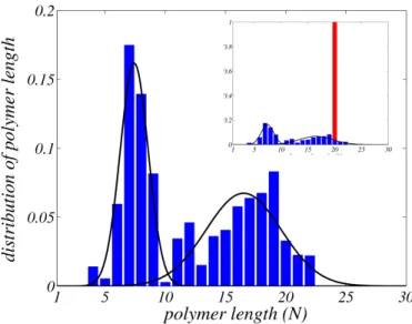
in 4,8,11. Our findings are clearly displayed in Fig. 3.
Figure 3. Distribution of polymers length after 4500 divisions (blue), starting with 5 identical protocells with polymer length of 20 monomers (red) (shown in the inset). Two species are clearly identified corresponding to the 47.3 % and 52.7 % of the whole popu-lation, resulting from the selection of the fittest mutated protocells, in the competition for food. The solid black lines are the results of numerical interpolations: one Gaussian curve has mean 7.4 and standard deviation 1.1, while the second one is centered at 16.5 with standard deviation 3.1. This picture represents a generic evolution: distinct runs relative to different choices of the parameters results in similar behaviors. Our findings are also shown to be robust to small changes of the parameters involved.
The occurrence of a speciation mechanism in a Chemoton–like pop-ulation is here demonstrated and contributes to shed new light into the important issue of protocells evolution and dynamics. In conclusion, and back to the initial question mutuated by G´anti, our modified Chemoton hy-pothesis defines not only a reliable unit of life, but also a unit of evolution. Importantly, this scenario does not apply to the original Chemoton de-scription, the geometrical aspects related to the process of division playing a fundamental role.
Acknowledgments
The first author whish to thank the funding of PACE (Programmable Ar-tificial Cell Evolution), an European Integrated Project in the EU
FP6-IST-FET Complex Systems Initiative under contract FP6-002035. Also I. Poli and R. Serra are acknowledged for useful comments and discussions. The numerical codes are implemented in matlab and can be delivered upon request.
Appendix A.
The aim of this Appendix is to provide further insight into a number of technical issues that have not been included in the main text to lighten the presentation. In particular, we shall focus on two specific topics: (i) mathematical representation of the membrane profile, computation of the associate volume and discussion of its role in our numerical experiments; (ii) protocols adopted in the numerical simulations.
Appendix A.1. Mathematical model of the protocell membrane
The aim of this section is to provide a detailed mathematical description of the membrane envelope that we have assumed in our study. First, let us recall the constraints that have to be verified:
(1) Immediately after a division event has occurred, each offspring has a small surface S0 and it can be ideally assimilated to a sphere. In
our simulations we set S0= 1.
(2) The successive division takes place once the protocell under scrutiny has essentially doubled its surface with respect to its original value. In other words, there exists a specific time T such that S(T ) = 2S0.
As soon as this steric condition is fulfilled, the protocells divides and generates two identical offspring.
(3) From the chemical equations of Table 2, one can infer the concen-tration of the membrane molecules, thus enabling us to calculate the corresponding size of the surface, through an ad hoc propor-tionality constant. The volume enclosed can be estimated once a specific shape of the container is imposed, the latter providing a unique relation between the surface size and the inner volume. (4) To mimic the effect played by the division mechanism on the
in-ner concentrations, we assume that a pinch region will eventually develop (as observed in real cells), the latter being related to the physical instability that initiates the division process. Practically, we shall hypothesize that the protocell progressively deform itself
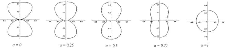
and finally assume an hourglass shape at the division time. This evolution is pictorially represented in the left panel of Fig. 2. Mathematically we adopted the following description. Let a be a real parameter belonging to the interval [0, 1] and introduce the following func-tions: ha(z) = s −az2+ r (1 − a)(z2− z4) +a 2S2 0 16π2and r(a) = v u u t1 − a + q (1 − a)2+a2S02 4π2 (a2− a + 1) 2(a2− a + 1) .
Then as a varies in between [0, 1], the rotation body with Cartesian equations:
x2+ y2= (ha(z))2and |z| ≤ r(a) ,
exhibits the desired properties. For a = 1, it corresponds to a sphere with surface S0; conversely, when a = 0 an hoursand–like profile is obtained.
In-termediate values of a enable to achieve a continuous transition in between the two aforementioned states. This is in turn confirmed by inspection of Fig. 4, where vertical sections are plotted for several values of a.
Figure 4. Vertical sections of the rotated body corresponding to distinct values of the parameter a.
Thanks to the Pappus Guldino Theorems f, for any given a, one can
calculate the surface and the volume associated to the 3D profile obtained above. The following explicit formula are derived:
Sa= 4π Z r(a) 0 ha(z) q 1 + (h′ a(z)) 2 dz and Va= 2π Z r(a) 0 (ha(z))2dz .
fThe first Theorem of Pappus Guldino states that the area of a surface of revolution
generated by rotating a plane curve γ about an axis external to γ and on the same plane is equal to the product of the arc length ℓ of γ and the distance d1traveled by its
centroid. The second Theorem of Pappus Guldino states that the volume of a solid of revolution generated by rotating a plane figure F about an external axis is equal to the product of the surface area of F and the distance d2traveled by its geometric centroid.
To fulfill the above requirements we further impose:
a = 2 − S(t)S
0 .
Hence, at t = 0, when S(0) = S0, a is equal to 1 and the corresponding
shape is a sphere, with unitary surface area. On the contrary, when S(t) = 2S0, then one gets a = 0, thus resulting in a hoursand profile. Still, the
surface area associated to the final hoursand-like state is not equal to 2S0.
To satisfy this latter condition, we can eventually deform the rotation body following the prescription reported below. Let
l(a) = r Sa 2 − aand fa(z) = ha(l(a)z) l(a) ,
then it can be shown that the rotation body defined in Cartesian coordi-nates by:
x2+ y2= (fa(z))2 and |z| ≤
r(a) l(a), matches the required conditions.
The obtained analytical expression of the membrane volume can be directly used into the relevant kinetic equations Eq. 1. Since chemical equations provides us with the time evolution of the outer surface, we choose to explicitly introduce the dependence of the volume vs. the surface and therefore write: V = f (S), where f represents the so called shape functiong.
The kinetic equations are hence modified as: dci dt = fi(¯c) − ci f′(S(t)) f(S (t )) dS (t ) dt , where f′ stands for the derivative of f with respect to S.
This term plays an essential role in our model: it enables in fact to significantly reduce the discontinuities arising at the division, as we shall discuss in the following. In Fig. 5 we report the results of two typical runs respectively relative to our improved formulation and to the original Ganti model. We focus in particular on the appearance of the discontinuities at division. Both runs refer to the same initial data and parameters choice (for the details of the integration scheme please refer to the next section). As clearly displayed, large jumps of the concentration are found in the sphere–shaped model, the gaps being almost eliminated when our picture gLet us note that for the case of a sphere f (S) = (6√π)−1S3/2.
is assumed to hold. This observation suggests that our formulation is indeed more realistic, hence correct, than the spherical–shaped one.
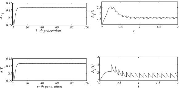
1 20 40 60 80 100 0.09 0.1 0.11 0.12 i−th generation ∆ T i 0 0.5 1 1.5 2 1.5 2 2.5 t A 1 (t) 0 20 40 60 80 100 0.09 0.1 0.11 0.12 i−th generation ∆ T i 0 0.5 1 1.5 2 1 2 3 4 t A 1 (t)
Figure 5. Upper panels: The hourglass shape model. On the left: the division time in function of the generation number for 100 successive divisions; observe that after a short transient the division time becomes independent on the division number and eventually reaches its asymptotic value: the division period (here 0.11359 units of time). On the right: the concentration of A1vs. time, during the first 16 divisions. Once again
after a short transient,the initial concentration reaches an asymptotic constant value (here, 1.5972 units of concentrations). Lower panels: the sphere shape model. On the left: the division time in function of the generation number, which exhibits almost the same behavior as before. In fact, it reaches the same asymptotic value 0.11359 in time–units. On the right: the concentration of A1 vs. time. Again, the qualitative
behavior resembles the former one, but the asymptotic value is lower: 1.3747 conc.–units. Observe the large jumps in the concentration value at the division step.
Appendix A.2. Protocol for a typical numerical simulation The numerical results presented in Fig. 5 are obtained by integrating the kinetic equations of Table 2. The aim of this section is to present the typical protocol used in our numerical experiments.
First, the parameters have to be assigned. For the reactions constants we adopted the values proposed by G´anti 7 and always used in the past
literature. Their nominal values are reported in Table 3. Observe that G´anti introduced these values being inspired to the following, general, cri-teria: (i) the direct reactions constants must be larger that the inverse ones, to emphasize a privileged direction for the chemical reactions; (ii) for these specific values G´anti demonstrated numerically the existence of peri-odic solutions. As concerns our current investigation, the first motivation is indeed important. On the contrary, we will show that by varying the other parameters involved, while keeping the same values for the reactions constants, one can eventually observe irregular behaviors.
Secondly, one needs to fix the parameters related to the double–stranded template (namely the associated length and polymerization threshold) and the available external food. The simulations reported in Fig. 5, and other reported in the previous sections are obtained by imposing:
N = 25 , V∗= 35.0 and ¯X = 100.0 . (A.1)
Finally, the initial concentrations of all the chemicals have to be set. Once again, and motivated by a preliminary analysis2of the configurations
space, we decided to resort to the original values proposed by G´anti and reported in Table 4.
Once all the above parameters and initial concentrations are assigned, and the maximal number of cycles specified, the kinetic equations are solved using the ode45 code in Matlab 10 V.6.5.1.199709 Rel. 13.1. When the surface size reaches the critical value S(T ) = 2.0, we “operate”the division and the halving of the inner materials accumulated during the evolution: the surface size is reset to the initial value S(T+) = 1.0, the concentrations
are rescaled by a shape factor, in our case ∼ 0.9408, which accounts for the fact that we re-initiate the subsequent evolution from a sphere-like state (the discontinuities seen in the top right panel of Fig. 5). The method proceeds with the subsequent iteration step.
A last remark concerns the construction of the State Function. The procedure just outlined allows us to numerically construct an orbit of a single protocell. Hence we are in a position to analyze the sequence of successive division times (see Fig. 1 or top left panel of Fig. 5) and determine whether the associated behavior is regular or not. Fixing all the quantities but the ones of Eq. A.1, one can construct a State Function as follows. For several values of ¯X and for each couple (N, V∗) defined over a large grid,
10 division times after a large transient of about 100 division cycles. For instance referring to Fig. 1 we associate to the values ¯X = 100.0, N = 25 and V∗ = 35.0 the value for the State Function:
F100.0(35.0, 25) = (0.1136, 0.1136, 0.1136, 0.1136, 0.1136, 0.1136
, 0.1136, 0.1136, 0.1136, 0.1136) ,
namely the orbit is regular: all the division time are equal. While in corre-spondence to values ¯X = 100.0, N = 25 and V∗= 42.9 the State Function
is now:
F100.0(42.9, 25) = (0.1205, 0.1081, 0.1168, 0.1091, 0.1209, 0.1080
, 0.1163, 0.1093, 0.1213, 0.1079) ,
the last 10 divisions have all a different duration, hence the orbit is irregular. We can obtain a rough idea of the behavior of the State Function, by plotting for fixed value of ¯X, N and V∗, the mean value of the last 10
computed division times. This is reported in Fig. 6 where a color code has been associated to the division time, to emphasize the regular and non– regular behavior we draw in blue each non–regular orbit.
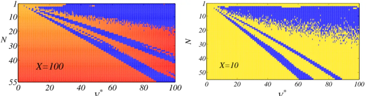
1 10 20 30 40 55 0 20 40 60 80 100 N V* X=100 0 20 40 60 80 100 1 10 20 30 40 50 V* N X=10
Figure 6. State Function. We report the State Functions obtained for different values of ¯X – on the left ¯X = 100.0 on the right ¯X = 10.0 – in a typical setting. Colors are assigned according to the classification into regular and irregular behaviors: blue dots refer to irregular ones, whereas regular orbits are represented in red–yellow, the faster the division period the lighter the color-coding. Some key qualitative features are always detected: domains of parameters (N, V∗) corresponding to regular and irregular
behaviors coexist, being particularly well mixed in correspondence of specific zones. This peculiar pattern is of paramount importance and intrinsically relates to the speciation mechanism.
Once several State Functions are stored, we can eventually simulate an open–ended Darwinian evolution, monitoring the dynamical response of a population under the pressure of the surrounding environment.
References
1. B. Alberts, A. Johnson, J. Lewis, M. Raff, K. Roberts & P. Walter , Molecular Biology of the Cell, New York, Garland, (2002).
2. T. Carletti, submitted, (2006).
3. T. Carletti & D. Fanelli, submitted, (2006).
4. F.M. Cohan, Annu. Rev. Microbiol., 56, pp. 457–487, (2002). 5. M. Eigen and P. Schuster, Naturwiss., 64, pp. 541–565, (1977). 6. T. G´anti, Biogenesis itself, J. theor. Biol., 187, pp. 583–593, (1997).
7. T. G´anti, I) Theory of Fluid Machineries & II) Theory of Living Systems, New York, Kluwer Academic/Plenum Publishers, (2003).
8. T.K. Konstantinidis & J.M. Tiedje, PNAS, 102, 7, pp. 2567–2572, (2005). 9. P.L. Luisi, F. Ferri & P. Stano, Naturwiss., 93, pp. 1–13, (2006).
10. Matlab, The language of technical computing, http://www.mathwork.com, (2006).
11. E. Moreno, Rev. Biol. trop., 50, 2, pp. 803–821, (2002).
12. A. Munteanu & R.V. Sol´e, J. Theor. Biol., 240, pp. 434–442, (2006). 13. S. Rasmussen, L. Chen, B. Stadler & P. Stadler, Origins Life & Evol. Biosph.,
34, pp. 171–180, (2004).
14. S. Rasmussen, L. Chen, D. Deamer, D.C. Krakauer, N.H. Packard, P.F. Stadler & M.A. Bedau, Science, 303, pp. 963–965, (2004).
15. E. Szathm´ary and J. Maynard Smith, J. Theor. Biol., 187, pp. 555–571, (1997).
16. E. Szathmary, M. Santos & C. Fernando, Topics in Current Chemistry, 259, pp. 167–211, (2005).
17. J. Singer & G.L. Nicolson, Science, 175, pp. 720–731, (1972). 18. D. Szostak, P.B. Bartel & P.L. Luisi, Nature, 409, 387–390, (2001).
Table 1. Chemoton Hypothesis. The chemical reactions describing the three cou-pled chemical subsystems.
Metabolism Membrane Template A1+ ¯X k1 GGGGGGGB FGGGGGGG k′ 1 A2 T′ k8 GGGGGGGAT ∗ pV 2N+ V′ k6 GGGGGGGB FGGGGGGG k′ 6 (pV2NpV1) + R A2 k2 GGGGGGGB FGGGGGGG k′ 2 A3+ ¯Y T∗+ R k9 GGGGGGGB FGGGGGGG k′ 9 T (pV2NpVi) + V′ k7 GGGGGGGA(pV2NpVi+1) + R A3 k3 GGGGGGGB FGGGGGGG k′ 3 A4+ V′ (pV2NpV2N)GGGGApV2N+ pV2N A4 k4 GGGGGGGB FGGGGGGG k′ 4 A5+ T′ A5 k5 GGGGGGGB FGGGGGGG k′ 5 A1+ A1
Note: In the first column the Autocatalytic Cycle A1→ 2A1is reported, the second
one focuses on the the membrane growth and the latter accounts for the template duplication. Here pV2N denotes the double stranded template constituted of 2N
monomers V′, whereas (pV
2NpVi), i = 1, . . . , 2N −1, denotes a partially duplicated
polymer where i–monomers have been copied. Direct reaction constants, kj, are
larger than the inverse ones, k′
j. We also assume the so-called strong replication
condition12to hold true: k
6, k′6and k7are zero if the concentration of V′is below
a given threshold V∗. The numerical values for the kinetic constants are set equal
1 1 :3 4 P ro ce ed in g s T ri m S iz e: 9 in x 6 in C a rl et ti F a n el liB IO M A T 2 0 0 6 ˙r ev
Table 2. Kinetic differential equations. From the chemical reactions one deduces the differential equations describing
the time evolution of the concentrations of the involved chemicals. To lighten notations, we denote the concentrations with capital letters.
Metabolism Membrane Template
˙ A1= 2`k5A5− k′5A21 ´ − k1A1X + k¯ 1′A2 T˙′= k4A4− k4′A5T′− k8T′ pV˙ 2N= 2k7(pV2NpV2n−1)V′ +k′ 6(pV2NpV1)R − k6pV2NV′ ˙ A2= k1A1X − k¯ ′1A2− k2A2+ k2′A3Y¯ T˙∗= k8T′− k9T∗R + k9′T (pV2N˙pV1) = k6pV2NV′− k′6(pV2NpV1)R −k7(pV2NpV1)V′ ˙ A3= k2A2− k2′A3Y − k¯ 3A3+ k′3A4V′ T = k˙ 9T∗R − k′9T − k10T S (pV2N˙pVi+1) = k7(pV2NpVi)V′ −k7(pV2NpVi+1)V′ ˙ A4= k3A3− k′3A4V′− k4A4+ k4′A5T′ S = k˙ 10T S V˙′= k3A3− k3′A4V′+ k6′(pV2NpV1)R −k6pV2NV′− k7P2N−1i=1 (pV2NpVi)V′ ˙ A5= k4A4− k′4A5T′− k5A5+ k5′A21 R = k˙ 6pV2NV′− k′6(pV2NpV1)R + k′9T −k9T∗R + k7P2N−1i=1 (pV2NpVi)V′
Note: The last equation in the middle column describes the growth of the surface size as a result of the progressive
Table 3. Reaction Constants.
k1= 2.0 k2= 100.0 k3= 100.0 k4= 100.0 k5= 10.0 k6= 10.0 k7= 10.0 k9= 10.0
k′
1= 0.1 k′2= 0.1 k3′ = 0.1 k′4= 0.1 k′5= 0.1 k′6= 1.0 k8= 10.0 k9′ = 0.1
k10= 10.0
Note: The reactions constants used in our simulations are reported. They refer to the original choice in7.
Table 4. Initial concentrations of involved chemicals.
A1(0) = 1.0 A2(0) = 1.8 A3(0) = 1.9 A4(0) = 1.7 A5(0) = 10.0 V′(0) = 26.0
T∗(0) = 14.0 T (0) = 0.0 R(0) = 0.0 Y (0) = 0.1¯ pV
2N(0) = 0.01 T′(0) = 17.0
S(0) = 1.0
Note: The table reports the initial concentrations of the chemicals involved in the chemical reactions. Ai(0), with i = 1, . . . , 5 are the chemicals taking part to the metabolic cycle;
V′ is the concentration of free monomers; T , T′ and T∗denote respectively the membrane
molecules and two kinds of precursors; R is a byproduct of the polymerization; ¯Y is the “waste”produced by the metabolic cycle; pV2N is the concentration of the double–stranded