Online optimization and learning in games: Theory and applications

HAL Id: tel-02428077

https://hal.inria.fr/tel-02428077

Submitted on 4 Jan 2020

HAL is a multi-disciplinary open access

archive for the deposit and dissemination of

sci-entific research documents, whether they are

pub-lished or not. The documents may come from

teaching and research institutions in France or

abroad, or from public or private research centers.

L’archive ouverte pluridisciplinaire HAL, est

destinée au dépôt et à la diffusion de documents

scientifiques de niveau recherche, publiés ou non,

émanant des établissements d’enseignement et de

recherche français ou étrangers, des laboratoires

publics ou privés.

applications

Panayotis Mertikopoulos

To cite this version:

Panayotis Mertikopoulos. Online optimization and learning in games: Theory and applications.

Opti-mization and Control [math.OC]. Grenoble 1 UGA - Université Grenoble Alpes, 2019. �tel-02428077�

THEORY AND APPLICATIONS

panayotis mertikop oulos

Habilitation à Diriger des Recherches

RAPPORTEURS

jérôme b olte Toulouse School of Economics & Université Toulouse 1 Capitole

nicolò cesa-bianchi Università degli Studi di Milano

sylvain sorin Sorbonne Université

EX AMINATEURS eric gaussier Université Grenoble Alpes

josef hof bauer Universität Wien

anatoli juditsky Université Grenoble Alpes

jérôme renault Toulouse School of Economics & Université Toulouse 1 Capitole

nicol as vieille École des Hautes Études Commerciales de Paris (HEC Paris)

Université Grenoble Alpes École doctorale MSTII

Spécialité: Informatique et Mathématiques Appliquées Soutenue à Grenoble, le 20 décembre 2019

T

he aim of this document is to give a bird’s eye view of my research on multi-agentonline learning. I do not claim to be comprehensive in this endeavor; rather, my guiding principle was to be comprehensible.

This had two main consequences: First, I had to leave out a fair number of research topics that I find equally exciting but did not otherwise fit the core of the present narrative. Second, I opted for a more conversational style, putting more emphasis on the results themselves rather than the technical trajectory that led to them. This might frustrate some readers who would seek to dive in the murky waters of the proofs and to analyze the technical contributions therein. I hope these readers will be satisfied by the list of references provided throughout this manuscript, and where all the relevant technical content can be found. Instead, my goal was to make the material presented herein accessible to non-experts in the field, to present a coherent narrative, and to explain what drives my research in these topics.

Chapter 2 is perhaps the clearest embodiment of this principle: it does not contain any original results per se, but rather intends to set the stage for the analysis to come. It reflects personal views – and biases – on the fundamentals of online learning and game theory, and I found it necessary to properly structure and position the rest of this document.

Chapters 3 and 4 comprise the theoretical backbone of my work and are aligned along two basic axes: continuous- vs. discrete-time considerations. From a practical viewpoint, the latter is often considered more interesting than the former: a system of stochastic differential equations can hardly be considered an implementable algorithm, and one could argue that modeling computer-aided decision processes as continuous-time dynamical systems is folly (on the surface at least). However, from a mathematical standpoint, the continuous- and discrete-time approaches comprise two synergistic research thrusts that dovetail in a unique and singular manner. Thanks to the theory of stochastic approximation (the glue that holds much of this manuscript together), insights gained in continuous time can be used to prove discrete-time results that would otherwise be inaccessible.

Chapters 5 and 6 focus on some applications of my work to high-performance com-puting (Chapter 5) and wireless communications (Chapter 6). I hesitated for a long time which applications to present and with what criteria to select them. In the end, I chose to focus on distributed computing and wireless networks because they were the closest in spirit to the material presented in the previous chapters, and because they provide an ideal playground for the theory developed therein. This meant that I had to leave out other equally interesting applications on generative adversarial networks and traffic routing, but this couldn’t be helped.

Finally, Chapter 7 presents some perspectives and directions for future research that arise naturally from the body of work preceding it. If the style of the previous chapters can be characterized as conversational, this last chapter is one of vigorous hand-waving, aiming to find a light switch in the dark. The questions stated therein are of a fairly open

Finally, Appendices A and B provide a series of biographical and bibliographical information. This is mostly intended to give some perspective of how the various ideas and questions evolved over time, and to provide some pointers to papers that treat a number of questions that could not be properly addressed within the rest of this manuscript.

discl aimer. Before proceeding, I would feel remiss not to point out that this manuscript is neither complete nor comprehensive – nor does it purport to be. I have tried to provide pointers to the relevant literature throughout, but it is not possible to do an adequate (let alone comprehensive) survey of the state of the art for all the topics addressed herein. The interested reader should be fully aware of this and should treat this manuscript as an entry point to a much wider literature.

T

he road leading to this document was long, full of turns and twists, and with its fairshare of dead ends and disappointments. What I feel made this journey worthwhile was what I got from my friends and colleagues along the way.

First and foremost, I need to express my deep gratitude to Jérôme Bolte, Nicolò Cesa-Bianchi, and Sylvain Sorin, the rapporteurs of this HDR. They generously contributed an immense amount of time reviewing this manuscript in detail, and their keen and insight-ful remarks were invaluable. I am similarly thankinsight-ful to my examinateurs, Eric Gaussier, Josef Hofbauer, Anatoli Juditsky, Jérôme Renault, and Nicolas Vieille: sacrificing their time and energy to make the trip to Grenoble in the middle of a nation-wide railway strike is, perhaps, the least reason for which I am grateful to all of them.

Of course, this document would never have existed without my extended academic family, their continued input, and their drive. I am particularly grateful to Rida for his constant bombardment of ideas over the years; to Veronica for her endless enthusiasm and vigor; to Bill for his unsurpassed mastery of game dynamics, matched only by his attention to detail; to Marco and Roberto for being role models of clarity and depth of thought; to Zhengyuan and Mathias for relentleslly pushing the boundary of the envelope; to all my co-authors for the countless lively exchanges and enriching discussions over the years; to my students and post-docs (Amélie, Olivier, Kimon, Yu-Guan,. . . ) for all the things they taught me; and to my colleagues in Grenoble (Arnaud, Bary, Bruno, Franck, Jérôme, Patrick,. . . ) for providing an ideal environment to work in.

Last but not least, I need to devote a special thanks to my parents, Kallia and Vlassis, my sister Victoria, and to my closest friends (Alex, Athena, Daniel, Lenja, Marios,. . . ) for their endless support and encouragement. Most of all however, I want to thank my wife, Tonia, for generously carrying me through all these sleepless nights, for keeping me tethered to reality, and for lovingly reminding me that the darkest hour is just before the dawn. All this is for her.

financial supp ort. My research was partially supported by the French National Research Agency (ANR) under grants ORACLESS (ANR-16-CE33-0004-01) and GAGA (ANR-16-13-JS01-0004-01), the Huawei Flagship Program ULTRON, and the EU COST Action CA16228 “European Network for Game Theory” (GAMENET). For a complete list of awarded grants, see Appendix A.

preface v

acknowled gments vii index xi

of figures xi of tables xi of algorithms xi of acronyms xii

of relevant publications xiv 1 introduction 1

1.1 Context and positioning 1 1.2 Diagrammatic outline 2 1.3 Notation and terminology 3

part i

theory

5

2 preliminaries 7

2.1 The unilateral viewpoint: online optimization 7 2.1.1 The basic model 7

2.1.2 Regret and regret minimization 9 2.2 No-regret algorithms 12

2.2.1 Feedback assumptions 12 2.2.2 Leader-following policies 14 2.2.3 Online gradient descent 16 2.2.4 Online mirror descent 18

2.2.5 Dual averaging and the link between FTRL and OMD 21 2.3 The multi-agent viewpoint: games and equilibrium 24

2.3.1 Basic definitions and examples 25 2.3.2 Nash equilibrium 27

2.3.3 Correlated and coarse correlated equilibrium 29 3 learning in games: a continuous-time skeleton 33

3.1 Learning dynamics 33 3.2 No-regret vs. convergence 37

3.2.1 Regret minimization 37

3.2.2 Cycles, non-convergence, and Poincaré recurrence 37 3.3 Convergence to equilibrium and rationalizability 39

3.3.1 Positive results in finite games 39 3.3.2 Positive results in concave games 41 3.4 Learning in the presence of noise 42

3.4.1 Single-agent considerations 44 3.4.2 Multi-agent considerations 46

4 learning in games: algorithmic analysis 51 4.1 No-regret vs. convergence: a discrete-time redux 51

4.1.1 Regret minimization 51

4.1.2 Limit cycles and persistence of off-equilibrium behavior 53 4.2 Convergence to equilibrium and rationalizability 55

4.2.1 Positive results in concave games 55

4.3.1 Payoff-based learning in concave games 60 4.3.2 Payoff-based learning in finite games 64

part ii

applications

67

5 distribu ted optimiz ation in multiple-worker systems 69 5.1 Multiple-worker systems 69

5.1.1 Master-slave architectures 70

5.1.2 Multi-core systems with shared memory 71 5.1.3 DASGD: A unified algorithmic representation 71 5.2 Analysis and results 72

5.2.1 Nonconvex unconstrained problems 72 5.2.2 Convex problems 73

5.2.3 Numerical experiments 74

6 signal covariance optimiz ation in wireless net works 77 6.1 System model and assumptions 77

6.2 Matrix exponential learning 79

6.2.1 The matrix exponential learning algorithm 79 6.2.2 Performance guarantees 80

6.3 Numerical experiments in MIMO networks 81 7 perspectives 85

biblio graphy 89 appendix 97 a vitæ 99

Education and professional experience 99 Awards and distinctions 99

Grants and collaborations 100 Awarded grants 100

Participation in research projects and networks 101 Scientific stays abroad 101

Scientific and administrative responsibilities 102 Coordination activities 102

Editorial activities 102 Conference organization 103 Committees 103

Research supervision and teaching 103 Invited talks and tutorials 104

b publications and scientific ou tpu t 107 Working / Submitted papers 107

Journal papers 107

Conference proceedings 109 Software 112

Dissertations 112

Frontispiece “Bunt im Dreieck”, by Wassily Kandinsky (lithograph, 1927) iii Figure 1.1 A typical generative adversarial network (GAN) architecture 2 Figure 2.1 Sequence of events in online optimization 8

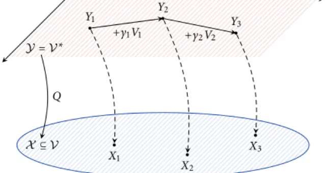
Figure 2.2 Schematic representation of online gradient descent 16 Figure 2.3 Schematic representation of dual averaging 22

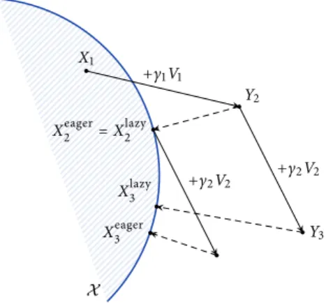
Figure 2.4 Lazy vs. eager gradient descent 23

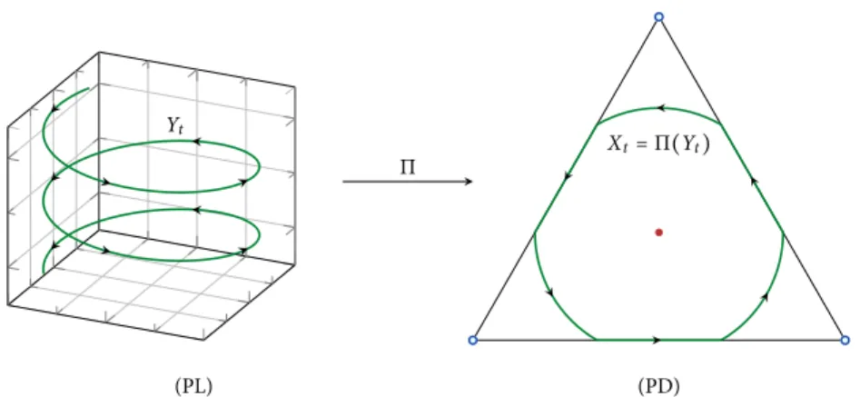
Figure 2.5 Variational characterization of Nash equilibria 28 Figure 3.1 The primal-dual relation between (PL) and (PD) 36

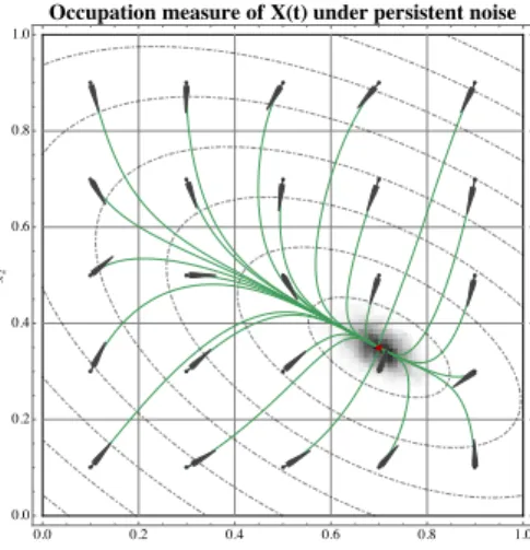
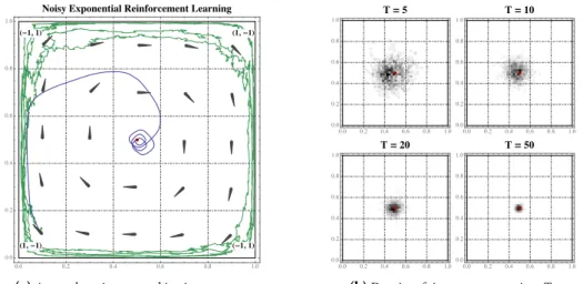
Figure 3.2 Cycles and recurrence of no-regret learning in zero-sum games 39 Figure 3.3 Long-run concentration of (SDA) around interior solutions 46 Figure 3.4 The long-run behavior of time-averages under (SDA) 48 Figure 4.1 Non-convergence of (DA) in zero-sum games 54 Figure 4.2 Dual averaging with bandit feedback 63

Figure 5.1 Convergence of DASGD in a non-convex problem 75 Figure 6.1 A MIMO multiple access channel network 78 Figure 6.2 Matrix exponential learning vs. water-filling 82 Figure 6.3 Scalability of matrix exponential learning 82

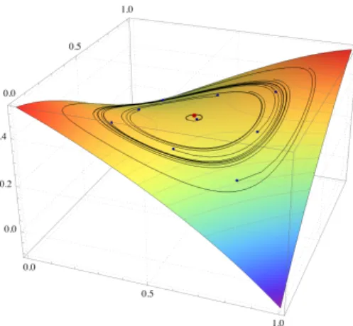
Figure 6.4 Wall-clock complexity of matrix exponential learning 83 Figure 7.1 Invariant measures in non-monotone saddle-point problems 87

LIST OF TABLES

Table 2.1 Regret achieved by (OGD) against L-Lipschitz convex losses 18

LIST OF ALGORITHMS

2.1 Follow the regularized leader 14

2.2 Online gradient descent 16

2.3 Online mirror descent 20

2.4 Dual averaging 22

4.1 Bandit dual averaging 62

4.2 EXP3 64

5.1 Master-slave implementation of stochastic gradient descent 70 5.2 Multi-core stochastic gradient descent with shared memory 71 5.3 Distributed asynchronous stochastic gradient descent 72

AI artificial intelligence APT asymptotic pseudotrajectory BDA bandit dual averaging BR best response

CCE coarse correlated equilibrium CE correlated equilibrium DA dual averaging

DASGD distributed asynchronous stochastic gradient descent DGF distance-generating function

DSC diagonal strict concavity EGD entropic gradient descent EGT evolutionary game theory ES evolutionary stability ESS evolutionarily stable state EW exponential weights

EXP3 exploration and exploitation with exponential weights FTL follow-the-leader

FTLL follow-the-linearized-leader FTRL follow-the-regularized-leader GAN generative adversarial network GD gradient descent

HPC high-performance computing HR Hessian–Riemannian IWF iterative water-filling KW Kiefer–Wolfowitz LGD lazy gradient descent LMD lazy mirror descent

i.i.d. independent and identically distributed ICT internally chain transitive

IS importance sampling LFP leader-following policy l.s.c. lower semi-continuous MAB multi-armed bandit MAC multiple access channel MD mirror descent

MIMO multiple-input and multiple-output

MW multiplicative weights MXL matrix exponential learning NE Nash equilibrium

NI Nikaido–Isoda OU Orstein–Uhlenbeck OGD online gradient descent OMD online mirror descent PI principal investigator

PPAD polynomial parity arguments on directed graphs RDP repeated decision problem

SDA stochastic dual averaging SDE stochastic differential equation SFO stochastic first-order oracle SGD stochastic gradient descent SP saddle-point

SPSA simultaneous perturbation stochastic approximation SVM suppport vector machine

SWF simultaneous water-filling VI variational inequality VLS very large scale VS variational stability WF water-filling

This manuscript contains contributions by the author from the papers listed below. More details can be found at the beginning of each section; a complete list of publications is presented in Appendix B.

[1] E. Veronica Belmega, Panayotis Mertikopoulos, Romain Negrel, and Luca Sanguinetti. On-line convex optimization and no-regret learning: Algorithms, guarantees and applications.

https://arxiv.org/abs/1804.04529_{, 2018.}

[2] Mario Bravo and Panayotis Mertikopoulos. On the robustness of learning in games with stochastically perturbed payoff observations. Games and Economic Behavior, 103, John Nash Memorial issue:41–66, May 2017.

[3] Mario Bravo, David S. Leslie, and Panayotis Mertikopoulos. Bandit learning in concave N-person games. In NIPS ’18: Proceedings of the 32nd International Conference on Neural Information Processing Systems, 2018.

[4] Johanne Cohen, Amélie Héliou, and Panayotis Mertikopoulos. Learning with bandit feedback in potential games. In NIPS ’17: Proceedings of the 31st International Conference on Neural Information Processing Systems, 2017.

[5] Johanne Cohen, Amélie Héliou, and Panayotis Mertikopoulos. Hedging under uncertainty: Regret minimization meets exponentially fast convergence. In SAGT ’17: Proceedings of the 10th International Symposium on Algorithmic Game Theory, 2017.

[6] Pierre Coucheney, Bruno Gaujal, and Panayotis Mertikopoulos. Penalty-regulated dynamics and robust learning procedures in games. Mathematics of Operations Research, 40(3):611– 633, August 2015.

[7] Joon Kwon and Panayotis Mertikopoulos. A continuous-time approach to online optimiza-tion. Journal of Dynamics and Games, 4(2):125–148, April 2017.

[8] Rida Laraki and Panayotis Mertikopoulos. Higher order game dynamics. Journal of Economic Theory, 148(6):2666–2695, November 2013.

[9] Rida Laraki and Panayotis Mertikopoulos. Inertial game dynamics and applications to constrained optimization. SIAM Journal on Control and Optimization, 53(5):3141–3170, October 2015.

[10] Panayotis Mertikopoulos and Aris L. Moustakas. The emergence of rational behavior in the presence of stochastic perturbations. The Annals of Applied Probability, 20(4):1359–1388, July 2010.

[11] Panayotis Mertikopoulos and Aris L. Moustakas. Learning in an uncertain world: MIMO covariance matrix optimization with imperfect feedback. IEEE Trans. Signal Process., 64(1): 5–18, January 2016.

[12] Panayotis Mertikopoulos and William H. Sandholm. Learning in games via reinforcement and regularization. Mathematics of Operations Research, 41(4):1297–1324, November 2016. [13] Panayotis Mertikopoulos and William H. Sandholm. Riemannian game dynamics. Journal

of Economic Theory, 177:315–364, September 2018.

[14] Panayotis Mertikopoulos and Mathias Staudigl. Convergence to Nash equilibrium in continuous games with noisy first-order feedback. In CDC ’17: Proceedings of the 56th IEEE Annual Conference on Decision and Control, 2017.

[15] Panayotis Mertikopoulos and Mathias Staudigl. On the convergence of gradient-like flows with noisy gradient input. SIAM Journal on Optimization, 28(1):163–197, January 2018. [16] Panayotis Mertikopoulos and Yannick Viossat. Imitation dynamics with payoff shocks.

International Journal of Game Theory, 45(1-2):291–320, March 2016.

2019.

[18] Panayotis Mertikopoulos, E. Veronica Belmega, and Aris L. Moustakas. Matrix exponential learning: Distributed optimization in MIMO systems. In ISIT ’12: Proceedings of the 2012 IEEE International Symposium on Information Theory, pages 3028–3032, 2012.

[19] Panayotis Mertikopoulos, E. Veronica Belmega, Aris L. Moustakas, and Samson Lasaulce. Distributed learning policies for power allocation in multiple access channels. IEEE J. Sel. Areas Commun., 30(1):96–106, January 2012.

[20] Panayotis Mertikopoulos, E. Veronica Belmega, Romain Negrel, and Luca Sanguinetti. Distributed stochastic optimization via matrix exponential learning. IEEE Trans. Signal Process., 65(9):2277–2290, May 2017.

[21] Panayotis Mertikopoulos, Christos H. Papadimitriou, and Georgios Piliouras. Cycles in adversarial regularized learning. In SODA ’18: Proceedings of the 29th annual ACM-SIAM Symposium on Discrete Algorithms, 2018.

[22] Panayotis Mertikopoulos, Bruno Lecouat, Houssam Zenati, Chuan-Sheng Foo, Vijay Chan-drasekhar, and Georgios Piliouras. Optimistic mirror descent in saddle-point problems: Going the extra (gradient) mile. In ICLR ’19: Proceedings of the 2019 International Conference on Learning Representations, 2019.

[23] Steven Perkins, Panayotis Mertikopoulos, and David S. Leslie. Mixed-strategy learning with continuous action sets. IEEE Trans. Autom. Control, 62(1):379–384, January 2017. [24] Luigi Vigneri, Georgios Paschos, and Panayotis Mertikopoulos. Large-scale network utility

maximization: Countering exponential growth with exponentiated gradients. In INFOCOM ’19: Proceedings of the 38th IEEE International Conference on Computer Communications, 2019.

[25] Zhengyuan Zhou, Panayotis Mertikopoulos, Nicholas Bambos, Stephen Boyd, and Peter W. Glynn. Stochastic mirror descent for variationally coherent optimization problems. In NIPS ’17: Proceedings of the 31st International Conference on Neural Information Processing Systems, 2017.

[26] Zhengyuan Zhou, Panayotis Mertikopoulos, Nicholas Bambos, Peter W. Glynn, and Yinyu Ye. Distributed stochastic optimization with large delays. Under review, 2018.

[27] Zhengyuan Zhou, Panayotis Mertikopoulos, Nicholas Bambos, Peter W. Glynn, Yinyu Ye, Jia Li, and Fei-Fei Li. Distributed asynchronous optimization with unbounded delays: How slow can you go? In ICML ’18: Proceedings of the 35th International Conference on Machine Learning, 2018.

[28] Zhengyuan Zhou, Panayotis Mertikopoulos, Nicholas Bambos, Stephen Boyd, and Peter W. Glynn. On the convergence of mirror descent beyond stochastic convex programming. SIAM Journal on Optimization, forthcoming.

1

INTRODUCTION

D

epending on the context, the word “learning” might mean very different things: innetwork science and control, it could mean changing the way resources are allocated for a particular task over time; in deep learning and artificial intelligence, it could mean training a neural network to discriminate between different objects in an image, or to generate new images altogether; in statistics, it could mean inferring the mapping from inputs to outputs in a complicated process (such as the response of a protein to a targeted stimulus); etc. The aim of this manuscript is to provide an in-depth look into the design and analysis of online learning algorithms in different contexts, both theoretical and applied: to examine what is and what isn’t possible, to analyze the interactions between different learning frameworks, and to provide concrete results that can be exploited in practice.

1.1 context and p ositioning

One common denominator that emerges in this highly diverse landscape is that learning invariably involves an agent that seeks to progressively improve their performance on a specific task – i.e., to “learn”. This agent – the “learner” – could be something as abstract as an algorithm (e.g., an artificial neural net), or something as mundane as a commuter going to work each day. Still, irrespective of the nature of the learner, learning is typically achieved via a feedback loop of the following general form:

1. The agent interfaces with their environment (a computer network, a dataset, etc.) by selecting an action (a resource allocation scheme, a weight configuration, etc.). 2. The agent receives some feedback based on the quality of the chosen action and the

state of the environment (e.g., the number of users in the network, the available datapoints, etc.).

An added complication to the above is that, in many practical applications, the actions of the learner may also affect the state of the environment, so this feedback loop might go both ways. This is perhaps best illustrated by two examples:

Example 1.1 (Traffic routing). Consider a set of computer users with a set of traffic

demands to be routed over a network (such as the Internet). If a user chooses to route a significant amount of traffic through a part of the network employed by other users, this part might become congested and users might end up switching to different routes. In so doing however, other, previously uncongested links might now become congested, so the first user would have to adapt to the new reality. In this way, every user in the network must both (i) learn which routes of the network are more suitable for their traffic demands; and (ii) learn to adapt to the behavior of other users that are simultaneously vying for the same resources.

Example 1.2 (Generative adversarial networks). A generative adversarial network (GAN)

is an artificial intelligence algorithm used in unsupervised machine learning to generate samples from an unknown, target distribution (e.g., images with sufficiently many

Figure 1.1: A typical GAN architecture and uncurated generated images taken from [102].

realistic characteristics to look authentic to human observers). Introduced in a seminal paper by Goodfellow et al. [56], a GAN consists of two neural networks competing against each other in a zero-sum game. One network – the generator – outputs candidate samples aiming to approximate the unknown target distribution, while the other network – the discriminator – evaluates the result based on a training set of instances taken from the true data distribution (for a schematic illustration, see Fig. 1.1). The objective of the generator is to fool the discriminator by providing samples that cannot be readily distinguished from the true distribution; at the same time, the discriminator seeks to adapt to the generator’s evolution over time. In this way, each network plays simultaneously the role of the “learner” and of the “environment” (to the other network).

Both examples above can be construed as special cases of multi-agent online learning:1 they comprise multiple interacting agents (or players), each with their individual actions, and seeking to attain possibly different objectives. As such, a fundamental question that arises in this context is the following:

Does learning lead to stability in multi-agent systems?

For instance, if all the users of a computer network follow a learning algorithm to try and learn the best route for their traffic demands, would that allow the system to converge to some “stable”, steady state?

1.2 diagrammatic ou tline

The rest of this manuscript aims to provide answers to this fundamental question in a range of different contexts, both practical and theoretical. For the reader’s convenience, we provide a rough diagrammatic outline below and we rely on a series of margin notes and hyperlinks to facilitate the navigation of the manuscript.

chap ter 2. We begin in Chapter 2 by providing a gentle introduction to online

Online optimization

and game theory _{optimization and game theory. The aim of this chapter is twofold: First, it represents}

an effort to make this manuscript as self-contained as possible by providing some fun-damental results in the field. Second, we aim to establish a point of reference for the analysis to come by collecting all relevant definitions, prerequisites, and basic no-regret algorithms (such as online gradient descent, online mirror descent / dual averaging, etc.). The reader who is already familiar with the material presented here can safely skip ahead and use it only as a reference for notation and terminology.

chapter 3. In this chapter, we flesh out a continuous-time skeleton for online

op-Continuous-time

analysis and results _{timization and learning in games. We discuss regret bounds in continuous time and}

how these overcome the corresponding minimax bounds for discrete time. We also

1 To maximize the number of applications treated in this manuscript, we do not revisit routing and GANs in the rest of this manuscript; for some of the author’s work on these topics, see instead [102, 147].

introduce a continuous-time dynamical system induced in multi-player games by the no-regret learning algorithms of Chapter 2, and we discuss some basic properties of these dynamics – both negative and positive. Specifically, we discuss (i) the dynamics’ Poincaré recurrence properties and their ramifications for convergence in zero-sum games (Section 3.2); (ii) the dynamics’ long-run convergence and rationalizability prop-erties, in both finite and continuous games (Section 3.3); and (iii) the robustness (and/or breakdown) of these properties in the presence of noise, modeled here as an Itô diffusion process (Section 3.4).

chapter 4. In Chapter 4, we return to the discrete-time, no-regret framework of Discrete-time

analysis and results

Chapter 2, and we examine which of the properties established in continuous time continue to hold in this bona fide algorithmic setting. More precisely, we discuss (i) the non-convergent behavior and the appearance of limit cycles under no-regret learning in zero-sum games in Section 4.1; (ii) the resolution of these phenomena in strictly monotone (or strictly coherent) games and games with dominated strategies or strict equilibria (Section 4.2); and (iii) the modifications to this analysis when the players of the game only have access to their in-game, realized payoffs (Section 4.3).

chapter 5. In this chapter, we examine a series of applications of the theory devel- Applications to

distributed optimization

oped in the previous chapters to the solution of very large scale distributed optimization problems. We consider different multi-worker configurations of computer clusters (master-slave architectures or multi-core systems with shared memory), and we focus on the optimization properties of a distributed implementation of stochastic gradient descent in this setting, Our main point of interest is the algorithm’s robustness to the delays incurred by different processors working at different speeds.

chap ter 6. Continuing with a series of applications of the theory developed in Applications to signal

processing

Chapters 3 and 4, we discuss in this chapter a game-theoretic / distributed optimization framework for the problem of throughput maximization in input and multiple-output systems. The main contribution outlined in this chapter is the derivation and analysis of the matrix exponential learning algorithm, an efficient solution method for trace-constrained semidefinite optimization problems. This algorithm is heavily influenced by the game-theoretic analysis of Chapter 4 and is shown to provide state-of-the-art guarantees for multi-antenna systems and networks.

Finally, Chapter 7 contains some perspectives and direction for future research, while Appendices A and B provide a series of biographical and bibliographical information for the author. For the reader’s convenience, we also provide a quick overview of the notational conventions used in this manuscript in the next section.

1.3 notation and terminolo gy

notational conventions. Throughout what follows,V will denote a finite-di- Convex analysis mensional real space with norm∥⋅∥ and X ⊆ V will be a closed convex subset thereof.

Following standard conventions, we will write ri(X ) for the relative interior of X , bd(X ) for its (relative) boundary, and diam(X ) = sup{∥x′_{− x∥ ∶ x, x}′_{∈ X } for its diameter.}

We will also writeY ≡ V∗for the (algebraic) dual ofV, ⟨y, x⟩ for the canonical pairing between y∈ Y and x ∈ V, and ∥y∥∗≡ sup{⟨y, x⟩ ∶ ∥x∥ ≤ 1} for the dual norm of y in Y.

Given an extended-real-valued function f∶ V → R ∪ {+∞}, its effective domain is defined as dom f = {x ∈ V ∶ f (x) < ∞} and its subdifferential at x ∈ dom f is given by ∂ f(x) = {y ∈ V∗ ∶ f (x′) ≥ f (x) + ⟨y, x′− x⟩ for all x′∈ V}. The doman of subdifferentiability of f is defined as dom ∂ f ≡ {x ∈ V ∶ ∂ f (x) ≠ ∅}. Finally, if ∂ f (x)

is a singleton, we will say that f is differentiable at x and we will write∇f (x) for the unique element thereof.

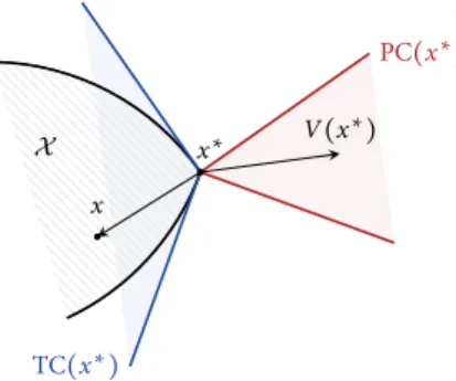
For all x∈ X , the tangent cone TCX(x) is defined as the closure of the set of all rays

emanating from x and intersectingX in at least one other point. Dually to the above, the polar cone PCX(x) to X at x is defined as PCX(x) = {y ∈ Y ∶ ⟨y, z⟩ ≤ 0 for all z ∈

TCX(x)}. For notational convenience, when X is understood from the context, we will

drop it altogether and write more simply TC(x) and PC(x) instead.

In the sequel, we will also make heavy use of the Landau asymptotic notationO(⋅),

Landau notation

o(⋅), Ω(⋅), etc. As a quick reminder, given two functions f , ∶ R → R, we say that f(t) = O((t)) if f grows no faster than , i.e., there exists some positive constant c > 0 such that∣f (t)∣ < c(t) for sufficiently large t (negative parts are ignored throughout). Conversely, we write f(t) = Ω((t)) if f grows no slower than , i.e., if (t) = O(f (t)). If we have both f(t) = O((t)) and f (t) = Ω((t)), we write f (t) = Θ((t)); and if limt→∞f(t)/(t) = 1, we say that  grows as f and we write f (t) ∼ (t) as t → ∞.

Finally, if lim sup_t→∞f(t)/(t) = 0, we write f (t) = o((t)) and we say that f is asymptotically dominated by .

a note on terminolo gy. There is an unfortunate disconnect between game

Descent vs. ascent

theory and optimization in terms of how objectives are formulated. In optimization, the objective is to minimize the incurred cost; in game theory, to maximize one’s re-wards. In turn, this creates a clash of terminology when referring to methods such as “gradient descent” or “mirror descent” in a maximization setting. To avoid going against the traditions of each field, we keep the usual conventions in place (minimization in optimization, maximization in game theory), and we rely on the reader to make the mental substitution of “descent” to “ascent” when needed.

Throughout this manuscript, we consider genderless agents and individuals. When

Epicenes

an individual is to be singled out, we will consistently employ the pronoun “they” and its inflected or derivative forms. The debate between grammarians regarding the use of “they” as a singular epicene pronoun (with different editions of The Chicago Manual of Style famously providing different recommendations) is beyond the scope of this manuscript.

2

PRELIMINARIES

O

ur aim in this introductory chapter is to discuss the basics of optimal decision-makingin unknown environments – what are the criteria for optimality, the policies that attain them, etc. To do so, we take an approach based on two complementary viewpoints. The first seeks to emulate the perspective of an agent that is faced with a recurring decision process but has no knowledge of its governing dynamics. We call this the “unilateral viewpoint” and we discuss it in detail in Sections 2.1 and 2.2. More precisely, Section 2.1 introduces the core framework of online optimization and the notion of regret which is central for our considerations; subsequently, in Section 2.2, we present an array of basic regret minimization algorithms and their performance guarantees.

The second viewpoint is more “holistic” and concerns several interacting agents whose decisions affect each other. The rules governing these interactions are still unknown to the agents, and the goal is to characterize those decisions that are simultaneously stable for each agent individually. We present this “multi-agent viewpoint” in Section 2.3: its main ingredients are non-cooperative games and the different solution concepts that arise in this context (Nash equilibrium, correlated equilibrium, etc.).

The natural bridging point between these two settings is the study of no-regret learning (a unilateral notion) in non-cooperative games (the quintessential element of the multi-agent viewpoint). This is the common unifying theme for most of this manuscript, and we examine it in detail in Chapters 3 and 4. The present chapter is meant to set the stage for the sequel by providing the core prerequisites for this analysis.

2.1 the unil ateral viewp oint : online optimiz ation

# This section incorporates material from the tutorial paper [13]

2.1.1 The basic model

Online optimization focuses on repeated decision problems (RDPs) where the objective Online optimization is to minimize the aggregate loss incurred against a sequence of unknown loss functions.

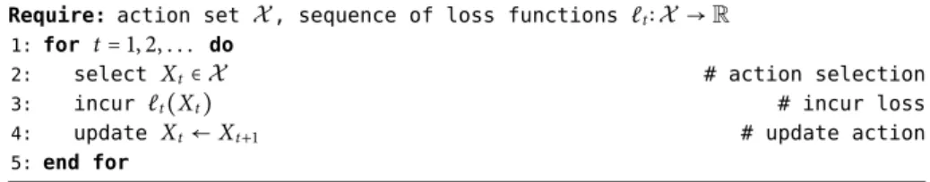
More precisely, the prototypical setting of online optimization can be summarized by the following sequence of events:

1. At every stage t= 1, 2, . . . , the optimizer selects an action Xtfrom a closed convex subsetX of an ambient n-dimensional normed space V.

2. Once an action has been selected, the optimizer incurs a loss ℓt(Xt) based on an

(a priori) unknown loss function ℓt∶ X → R.

3. Based on the incurred loss and/or any other feedback received, the optimizer updates their action and the process repeats.

Based on the structural properties of ℓt, we have the following basic problem classes: • Online convex optimization: each ℓtis assumed convex.

Require: action set X, sequence of loss functions ℓt∶ X → R

1: for t= 1, 2, . . . do

2: select Xt∈ X # action selection

3: incur ℓ_t(X_t) # incur loss

4: update X_t← X_t+1 # update action

5: end for

Figure 2.1: Sequence of events in online optimization.

• Online strongly convex optimization: each ℓtis assumed strongly convex, i.e., ℓt(x′) ≥ ℓt(x) + ⟨∇ℓt(x), x′− x⟩ +αt

2∥x

′_{− x∥}2

(2.1) for some αt > 0 (called the strong convexity modulus of ℓt).

• Online linear optimization: each ℓtis assumed linear, i.e., of the form

ℓt(x) = −⟨vt, x⟩ for some payoff vector vt∈ V∗. (2.2) Linear and strongly convex problems are both subclasses of the convex class, but they are otherwise disjoint; for convenience, we also assume throughout that each ℓt is differentiable1 and that it attains its minimum inX .

For concreteness, we discuss below some key examples of repeated decision problems (see also Fig. 2.1 for a pseudocode representation):

Example 2.1. Consider the static optimization problem Static optimization

minimize f(x)

subject to x∈ X (Opt)

where f∶ X → R is a static objective function. Viewed as an RDP, this corresponds to the case where the loss functions encountered by the optimizer are all equal to f , i.e.,

ℓt(x) = f (x) for all t = 1, 2, . . . (2.3) The optimality gap of a sequence of actions Xt∈ X after T stages is then given by

Gap(T) =∑T t=1f(Xt) − T minx∈X f(x) = T ∑ t=1ℓt(Xt) − minx∈X T ∑ t=1f(x) = max x∈X T ∑ t=1[ℓt(Xt) − ℓt(x)]. (2.4)

This last quantity is known as the agent’s regret and it plays a central role in the sequel.

Example 2.2. Extending the above to problems involving randomness and uncertainty, Stochastic optimization

consider the stochastic optimization problem

minimize f(x) ≡ E[F(x; ω)]

subject to x∈ X (Opt-S)

1 We adopt here the established convention of treating gradients as dual vectors. For book-keeping reasons, we will tacitly assume that ℓtis defined on an open neighborhood of X in V; alternatively, in the convex case, if we view ℓtas an extended-real-valued function on V with effective domain dom ℓt≡ {x ∈ V ∶ ℓ_t(x) < ∞} = X , we can simply assume that ∂ℓtadmits a continuous selection, denoted by ∇ℓt. Either way, none of the results presented in the sequel depend on this device, so we do not make this assumption explicit.

where F∶ X ×Ω → R is a stochastic objective defined on some probability space (Ω, F, P). In the RDP framework described above, it is assumed that an i.i.d. random sample ωt∈ Ω

is drawn at each stage t= 1, 2, . . . , and the loss function encountered by the optimizer is ℓt(x) = F(x; ωt) for all t = 1, 2, . . . (2.5) As a result, the best that the optimizer could do on average would be to play a solution of (Opt-S); in turn, this leads to the mean optimality gap

Gap(T) = E[∑T t=1ℓt(Xt)] − T minx∈X f(x) = E[ T ∑ t=1ℓt(Xt)] − minx∈XE[ T ∑ t=1F(x; ωt)] ≤ E[∑T t=1ℓt(Xt)] − E[minx∈X T ∑ t=1ℓt(x)] = E[max x∈X T ∑ t=1[ℓt(Xt) − ℓt(x)]]. (2.6)

Of course, if there is no randomness, this expression reduces to (2.4).

Example 2.3. As a third example, consider the saddle-point (SP) problem Saddle-point problems

minimize f(x) ≡ maxθ∈ΘΦ(x; θ)

subject to x∈ X (SP)

where θ is a parameter affecting the problem’s value function Φ∶ X × Θ → R in a manner beyond the optimizer’s control. In other words, (SP) simply captures Wald’s minimax optimization criterion of minimizing one’s losses against the worst possible instance (i.e., attaining a certain security level no matter what).

In the associated RDP, θt ∈ Θ is chosen at each stage t = 1, 2, . . . by an abstract

adversary, so the loss function encountered by the optimizer is

ℓt(x) = Φ(x; θt) for all t = 1, 2, . . . (2.7) Accordingly, the optimality gap relative to a minimax solution of (SP) is bounded as

Gap(T) =∑T t=1ℓt(Xt) − T minx∈X f(x) = T ∑ t=1ℓt(Xt) − T minx∈Xmaxθ∈ΘΦ(x; θ) ≤∑T t=1ℓt(Xt) − minx∈X T ∑ t=1Φ(x; θt) = T ∑ t=1ℓt(Xt) − minx∈X T ∑ t=1ℓt(x) = max_x∈X∑T t=1[ℓt(Xt) − ℓt(x)]. (2.8)

Again, this expression is formally similar to the corresponding expression (2.4) for static optimization problems; we elaborate on this relation below.

2.1.2 Regret and regret minimization

In each of the above examples, there is a well-defined solution concept which could be viewed as a natural target point of the associated RDP (minimizers of f in Example 2.1, average minimizers in Example 2.2, and minimax solutions in Example 2.3). In general however, these concepts may not be meaningful because, unless more rigid assumptions are in place, there may be no fixed target point to attain, either static or in the mean.

This limitation is overcome by the notion of regret, which dates back at least to the work of Blackwell [19] and Hannan [57] in the 1950’s:

Definition 2.1. The regret incurred by a sequence of actions Xt∈ X against a sequence

Regret

of loss functions ℓt∶ X → R, t = 1, 2, . . . , is defined as

Reg(T) = max_x∈X∑T t=1[ℓt(Xt) − ℓt(x)] = T ∑ t=1ℓt(Xt) − minx∈X T ∑ t=1ℓt(x) (2.9)

i.e., as the difference between the aggregate loss incurred by the agent after T stages and that of the best action in hindsight.

In words, the agent’s regret contrasts the performance of the agent’s policy Xtto that of an action x∗∈ arg min_x∈X∑Tt=1ℓt(x) which minimizes the total incurred loss over

the horizon of play. On that account, the main goal in online optimization is to design

No regret

causal, online policies that achieve no regret, i.e.,

Reg(T) = o(T) for any sequence of loss functions ℓt, t= 1, 2, . . . (2.10) The performance of such a policy is then evaluated in terms of the actual regret mini-mization rate achieved, i.e., the precise expression in the o(T) term above.

The situation becomes more complicated if the policy Xtis itself random – and, in particular, if its randomness is correlated to any randomness that might underlie ℓt. In

Expected regret and

pseudo-regret _{that case, the expected regret of a policy Xtis defined as}

E[Reg(T)] = E[max_x∈X∑T

t=1[ℓt(Xt) − ℓt(x)]]. (2.11)

This expression involves the expectation of a minimum which, in general, is difficult to compute. Instead, a more useful proxy for the regret in stochastic environments is the so-called pseudo-regret, defined here as

Reg(T) = max_x∈X E[∑T

t=1[ℓt(Xt) − ℓt(x)]] (2.12)

Since the maximum of the expectation of a family of random variables is majorized by the expectation of the maximum, we have

Reg(T) ≤ E[Reg(T)], (2.13)

so the pseudo-regret is tighter as a worst-case guarantee.

In a stochastic setting, it is more natural to target the optimal action in expectation rather than the action which is optimal against the sequence of realized losses. Moreover, by standard Chernoff–Hoeffding arguments, the typical difference between the expected regret and the pseudo-regret is of the order of Θ(√T). Thus, in general, one cannot hope to achieve an expected regret minimization rate better thanO(√T); by contrast, in several cases of interest, it is possible to attain much more refined bounds for the pseudo-regret. Because of this, Reg(T) will be our principal figure of merit for regret minimization in the presence of randomness and/or uncertainty.

We close this section by revisiting some of the previous examples:

Example 2.4. Going back to the static framework of Example 2.1, Eq. (2.4) yields Value convergence 1 T T ∑ t=1f(Xt) = min f + 1 TReg(T). (2.14)

Hence, if Xtis a no-regret policy, the sequence of function values f(Xt) converges to

min f in the Cesàro sense. In particular, if f is convex, Jensen’s inequality shows that the time-averaged sequence

¯ XT = _T1

T

∑

t=1Xt (2.15)

achieves the value convergence rate

f( ¯XT) ≤ min f +_T1 Reg(T). (2.16) Likewise, in the stochastic setting of Example 2.2, we readily obtain

E[f ( ¯XT)] ≤ min f +_T1 Reg(T) (2.17) provided that ωtis independent of Xt.2

This mode of convergence is often referred to as “ergodic convergence” or Polyak–Rup-pert averaging [117] and its study dates back at least to Novikoff [114]. In particular, if ¯XT

is viewed as the output of an optimization algorithm generating the sequence of states Xt∈ X , the induced (pseudo-)regret directly reflects the algorithm’s value convergence

rate. We will revisit this issue several times in the sequel.

Example 2.5. Consider the following discrete variant of the stochastic optimization Multi-armed bandits

setting of Example 2.2. At each stage t= 1, 2, . . . , the optimizer selects an action atfrom some finite setA = {1, . . . , n}. The reward of each arm a ∈ A is assumed to be an i.i.d. random variable va,t∈ [0, 1] drawn from an unknown distribution Pa, and the aim is to choose the action with the highest mean reward as often as possible. Following Robbins [119], this is called a (stochastic) multi-armed bandit (MAB) problem in reference to the “arms” of a slot machine in a casino – a “bandit” in the colorful slang of the 1950’s.

To quantify the above, let µadenote the mean value of the reward distribution Paof the a-th arm, and let

µ∗≡ max

a∈Aµa and a

∗_{≡ arg max}

a∈A µa (2.18)

respectively denote the bandit’s maximal mean reward and the arm that achieves it (a priori, there could be several such arms but, for simplicity, we assume here that there is only one). Then, if the agent selects a∈ A at time t with probability Xa,t, the induced (pseudo-)regret after T stages will be

Reg(T) = µ∗_T−∑T

t=1E[vat, t] = maxa∈A T ∑ t=1E[va,t− vat, t] = max x∈∆(A)E[ T ∑ t=1⟨vt, x− Xt⟩] = maxx∈∆(A)E[ T ∑ t=1[ℓt(Xt) − ℓt(x)]] (2.19)

where: (i) atdenotes the arm played at time t; (ii) vt = (va,t)a∈A ∈ Rnis the reward vector of stage t (typically it is assumed that−1 ≤ va,t ≤ 1 for all t); and (iii) the loss

functions ℓtare defined as ℓt(x) = −⟨vt, x⟩.3 Under this light, multi-armed bandits can

be seen as (linear) stochastic optimization problems over the simplexX ≡ ∆(A) of probability distributions overA.

2 Recall here that ωtis drawn after Xt, so this independence is not restrictive: for instance, this is always the case if ωtis i.i.d. and Xtis predictable relative to the history σ (ω1, . . . , ωt−1)of ωtup to stage t − 1. 3 Since each ℓtis linear in x, maximizing over A or ∆(A) gives the same result.

2.2 no-regret algorithms

# This section incorporates material from the tutorial paper [13]

We now turn to the fundamental question underlying the online optimization frame-work discussed above:

Is it possible to achieve no regret? And, if so, at what rate?

Of course, any answer to these questions must depend on the specifics of the problem at hand – the assumptions governing the problem’s loss functions, the information available to the optimizer, etc. In the rest of this section, we focus on obtaining simple answers in a range of different settings that arise in practice.

2.2.1 Feedback assumptions

We begin by specifying the type and amount of information available to the optimizer.

Oracle feedback

Our starting point will be the so-called “oracle model” in which the optimizer gains access to each loss function via a black-box feedback mechanism (i.e., in a model-agnostic manner). Formally, given a (complete) probability space(Ω, F, P) and a measurable space of signalsS, an oracle for a function f ∶ X → R is simply a map Orf∶ X × Ω → S

that outputs a (random) signal Orf(x; ω) ∈ S when called at x ∈ X . Some important

examples of such oracles are discussed below:

1. Full information: In this case, the space of signalsS is a space of functions and

Full information

Orf(x) = f . In other words, when called at a point x ∈ X , a full-information

oracle returns the entire function f∶ X → R (hence the name). [This oracle is assumed deterministic, so we suppress the argument ω.]

2. Perfect n-th order information: Oracles in this class return information on the n-th order derivates of the function at the input point x ∈ X . In the “perfect information” case, when called at x∈ X , the oracle returns the tensor

Orf(x) = Dnf(x) = ( ∂ n_f ∂xi1. . . ∂xin ) i1,..., in=1,...,n (2.20)

[Again, these oracles are assumed deterministic so the argument ω is suppressed.] By far the most widely used oracles of this type are the cases n= 0, 1 and 2:

• The case n= 0 gives Orf(x) = f (x) and is known in the literature as bandit

Bandit feedback

feedback (in reference to the multi-armed bandit problem of Example 2.5). It is most common in problems where scarcity of information plays a major role (such as adversarial and game-theoretic learning).

• The case n = 1 corresponds to perfect gradient feedback, i.e., Orf(x) =

Gradient feedback

∇f (x). This is most common in medium-to-small-scale optimization prob-lems where exact gradient calculations are still within reach.

• The case n= 2 amounts to accessing to the Hessian matrix Hess(f (x)) of f

Hessian feedback

at x. Hessian calculations are very intensive in terms of computational power, so such oracles are most commonly encountered in relatively small-scale optimization problems that need to be solved to a high degree of accuracy. 3. Noisy n-th order information: Here, the setup is as before with the difference that the output of the oracle is random. Specializing directly to the cases that are most common in practice, we have:

• The case n = 0 corresponds to noisy function evaluations of the form Noisy bandit feedback Orf(x; ω) = f (x) + ξ(x; ω) for some additive noise variable ξ ∈ R.

Or-acles of this type are the norm in bandit convex optimization problems and problems where even the calculation of the objective function is computa-tionally intensive.

• The case n= 1 provides noisy gradient evaluations of the form Orf(x; ω) = Noisy gradient feedback

∇f (x) + U(x; ω) for some observational noise variable U ∈ V∗_{. This type}

of feedback is extremely common in distributed optimization problems with objectives of the form f(x) = ∑N_i=1fi(x): taking a random sample

i∈ {1, . . . , N} (or a minibatch thereof) and calculating its gradient gives a stochastic first-order oracle that is widely used in machine learning, signal processing, and data science.

The informational content of an oracle can be gauged by the dimension of the signal Memory requirements spaceS, which in turn provides an estimate of the memory required to store and process

the received signal. In the full information case,S is typically infinite-dimensional, so such oracles are of limited practical interest (but are still very useful from a theoretical standpoint). At the other end of the spectrum, zeroth-order oracles haveS = R, so they are the lightest in terms of memory requirements (but are otherwise the hardest to work with). Between these two extremes, n-th order oracles haveS = (V∗)⊗n ≅ Rnn, i.e., their memory requirements grow exponentially in n. This “curse of dimensionality” is one of the main reasons for the sweeping popularity of first-order methods in problems where the dimension of the ambient state spaceV becomes prohibitively large.

In view of the above, a large part of our analysis will focus on stochastic first-order Stochastic first-order

oracle feedback

oracles (SFOs) that return possibly imperfect gradient measurements at the point where they are called. Specifically, we will assume that such an oracle is called repeatedly at a (possibly random) sequence of points Xt∈ X and, at each stage t = 1, 2, . . . , returns a

vector signal of the form

∇t= ∇ℓt(Xt) + Zt (2.21) where the “observational error” term Ztcaptures all sources of uncertainty in the oracle.

In more detail, to differentiate between “random” (zero-mean) and “systematic” (non- Random vs. systematic

errors

zero-mean) errors in∇t, it will be convenient to decompose Ztas

Zt= Ut+ bt (2.22)

where Ut is zero-mean and bt captures the mean value of Zt. To define these two processes formally, we will subsume any randomness in∇tand ℓtin a joint event ωt

drawn from some (complete) probability space(Ω, F, P). Since this randomness is generated after the optimizer selects an action Xt ∈ X (cf. the sequence of events in

Fig. 2.1), the processes∇tand Ztare, a priori, not adapted to the history of Xt. More explicitly, writingFt= σ(X1, . . . , Xt) for the natural filtration of Xt, the processes bt

and Utare defined as

bt= E[Zt∣ Ft] and Ut= Zt− bt (2.23) so, by definition, E[Ut∣ Ft] = 0.

In view of all this, SFOs can be classified according to the following statistics: SFO statistics 1. Bias:

Bt = E[∥bt∥∗] (2.24a) 2. Variance:

σ2

Algorithm 2.1: Follow the regularized leader

Require: strongly convex regularizer h∶ X → R; weight parameter γ> 0

1: for t= 1, 2, . . . do

2: play X← arg min_x∈X{∑t_s=1ℓs(x) + γ−1h(x)} # choose action

3: observe ℓ_t # get feedback

4: end for

3. Second moment:

M2

t = E[∥∇t∥∗2] (2.24c) An oracle with Bt= 0 for all t will be called unbiased, and an oracle with limt→0Bt= 0

will be called asymptotically unbiased; finally, an unbiased oracle with σt = 0 for all t will

be called perfect. We will examine all these cases in detail in the sequel.

2.2.2 Leader-following policies

The first no-regret candidate process that we will examine is based on the following

Follow the leader

simple principle: at time t+ 1, the optimizer plays the action that is optimal in hindsight up to (and including) stage t. This policy is known as follow-the-leader (FTL) and it can be formally described via the update rule:

Xt+1∈ arg min x∈X

t

∑

s=1ℓs(x) (FTL)

with the usual convention∑_t∈∅at = 0 for the empty sum (i.e., X1is initialized arbitrarily).

In terms of computational overhead, this policy requires a full information oracle

Cover’s impossibility

principle _{(i.e., the knowledge of ℓt once Xt is chosen) and the ability to compute the arg min}

in the (FTL) update rule. Both requirements are significantly lighter in online linear optimization problems where each objective is of the form (2.2). However, even in this restricted setting, (FTL) incurs positive regret: a well-known example overX = [−1, 1] is provided by the sequence of alternating losses

ℓt(x) =⎧⎪⎪⎪⎪⎨ ⎪⎪⎪⎪ ⎩ −x/2 for t= 1, x if t> 1 is even, −x if t> 1 is odd. (2.25)

Against this sequence, (FTL) gives Xt = arg minx∈[−1,1](−1)t−1x/2 = (−1)tfor all t > 1, so the total incurred loss after T stages is∑T_t=1ℓt(Xt) = T − X1/2 − 1. By contrast, the

constant policy Xt= 0 incurs zero loss for all t, implying in turn that Reg(T) ∼ T.

The main reason behind this failure is that (FTL) is too “aggressive”. Indeed, if the

Follow the

regularized leader _{cumulative loss function∑}t

s=1ℓsexhibits significant oscillations between one stage and the next, (FTL) will also jiggle between extremes, and this behavior can be exploited by the adversary. One way to overcome this behavior is to introduce a penalty term which makes these oscillations less extreme (and hence, less exploitable); this leads to a policy known as follow-the-regularized-leader (FTRL) [135–137], and which can be stated as follows: Xt+1= arg min x∈X { t ∑ s=1ℓs(x) + 1 γh(x)}. (FTRL)

[For a pseudocode implementation, see Algorithm 2.1.]

In the above, h∶ X → R is a regularization (or penalty) function and γ > 0 is a tunable parameter that adjusts the weight of the regularization term. By this token, to ensure

that this mechanism dampens oscillations, it is common to assume that the regularizer h∶ X → R is continuous and strongly convex, i.e., there exists some K > 0 such that

[λh(x′_{) + (1 − λ)h(x)] − h(λx}′_{+ (1 − λ)x) ≥} K

2λ(1 − λ) ∥x

′_{− x∥}2

(2.26) for all x, x′ ∈ X and all λ ∈ [0, 1]. Moreover, under the empty sum convention ∑0

s=1ℓs(x) ≡ 0, the method is initialized at the so-called prox-center xcofX , viz. X1= xc≡ arg min

x∈X h(x). (2.27)

Remark. We should state here that (FTL) and (FTRL) are closely related to the learning policies known in economics and game theory as fictitious play (FP) and smooth fictitious play (SFP) respectively. These policies correspond to playing a best response (resp. regularized or smooth best response) to the empirical history of play of one’s opponents, and their study dates back to Brown [29], Robinson [121], and Fudenberg and Levine [54]; for a more recent treatment, see also Hofbauer and Sandholm [65].

With all this in hand, the regret analysis of (FTRL) is typically performed under the Blanket assumptions following blanket assumptions:

Assumption 2.1 (Convexity). Each ℓt∶ X → R is convex.

Assumption 2.2 (Lipschitz continuity). Each ℓt∶ X → R is Lipschitz continuous, i.e.,

∣ℓt(x′) − ℓt(x)∣ ≤ Lt∥x′− x∥ (2.28) for some Lt> 0 and all x, x′∈ X .

Remark. Since ℓtis assumed differentiable, Assumption 2.2 basically provides an upper bound for its gradient. In the convex case, all this can be subsumed in the assumption that the subdifferential of ℓtonX admits a bounded selection. We will not require this level of detail at this point, so we stick with the simplest formulation.

In this general setting, we have the following basic result:

Theorem 2.1 (Shalev-Shwartz, 2007). Suppose that (FTRL) is run against a sequence of Regret of FTRL

loss functions ℓt, t = 1, 2, . . . , satisfying Assumptions 2.1 and 2.2. Then, the algorithm’s

regret is bounded by

Reg(T) ≤H_γ +_Kγ ∑T

t=1L 2

t (2.29)

where H≡ max h−min h denotes the “depth” of h over X .4 In particular, if L ≡ sup_tLt < ∞

and (FTRL) is run with regularization parameter γ= (1/L)√HK/T, the incurred regret is bounded as

Reg(T) ≤ 2L√(H/K)T. (2.30)

Theorem 2.1 shows that achieving no regret is possible as long as (i) the optimizer has full access to the loss functions ℓtrevealed up to the previous stage (inclusive); (ii) the minimization problem defining (FTRL) can be solved efficiently; and (iii) the horizon of play is known in advance. Of these limitations, (iii) is the easiest to resolve via a method known as the “doubling trick”;5 on the other hand, (i) and (ii) represent inherent limitations of leader-following policies and are harder to overcome. We address these points in detail in the next section.

4 We write here H instead HXfor notational simplicity.

5 In a nutshell, this involves running (FTRL) over windows of increasing length with a step-size that is chosen optimally for each window; for a detailed account, see Cesa-Bianchi and Lugosi [35], Shalev-Shwartz [136].

X X1 X2 X3 −γ₁∇₁ −γ₂∇₂

Figure 2.2: Schematic representation of online gradient descent.

Algorithm 2.2: Online gradient descent

Require: step-size sequence γt> 0

1: choose X₁∈ X # initialization

2: for t= 1, 2, . . . do

3: incur loss ℓ_t(X_t) # losses revealed

4: receive signal V_t← −[∇ℓ_t(X_t) + U_t] # oracle feedback

5: update X_t+1← Π(X_t+ γ_tV_t) # gradient step

6: end for

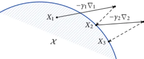
2.2.3 Online gradient descent

In optimization theory, the most straightforward approach to minimize a given loss

Online gradient descent

function is based on (projected) gradient descent: at each stage, the algorithm takes a step against the gradient of the objective, the resulting point is projected back to the problem’s feasible region (if needed), and the process repeats.

When faced with a different loss function at each stage, this gives rise to the policy known as online gradient descent (OGD). Formally, this refers to the recursive update rule

Xt+1= Π(Xt+ γtVt) (OGD) where

Vt= −∇t= −[∇ℓt(Xt) + Zt] (2.31) denotes the return of a stochastic first-order oracle at Xt(cf. Section 2.2.1), γt> 0 is the

algorithm’s step-size (discussed below), and Π∶ V → X is the Euclidean projector Π(x) = arg min

x′∈X

∥x′_{− x∥}2

. (2.32)

[For a schematic representation of the method, see Fig. 2.2; see also Algorithm 2.2 for a pseudocode implementation. For simplicity, we also drop the dependence of Π onX , and we write Π instead of ΠX.]

Remark 2.1. Before proceeding, it is worth noting a technical discrepancy in (OGD). Specifically, seeing as gradients are formally represented as dual vectors, the addition Xt+γtVtof a primal and a dual vector is not well-defined. This issue is usually handwaved away by assuming thatV is a Euclidean (or Hilbert) space, in which case V∗is canonically identified withV. However, this assumption can only be made if the norm ∥⋅∥ satisfies the parallelogram law (i.e., if it is induced by a scalar product); if this is not the case (e.g., if∥⋅∥ is the L1norm), the situation is more delicate. We discuss this issue in detail in the next section.

The study of (OGD) in online optimization can be traced back to the seminal paper of Zinkevich [157] who established the following basic bound:

Theorem 2.2 (Zinkevich, 2003). Suppose that (OGD) is run against a sequence of loss Regret of OGD

functions satisfying Assumptions 2.1 and 2.2 with a constant step-size γt≡ γ > 0 and SFO

feedback of the form (2.31). Then, the algorithm’s regret is bounded as Reg(T) ≤diam(X )2 2γ + γ 2 T ∑ t=1M 2 t + diam(X ) T ∑ t=1Bt (2.33)

where diam(X ) ≡ max{∥x′_{− x∥ ∶ x, x}′_{∈ X } denotes the diameter of X . In particular,}

if M ≡ suptMt < ∞ and (OGD) is run with step-size γ = (1/M) diam(X )/√T, the

algorithm enjoys the bound

Reg(T) ≤ diam(X )[M√T+∑T

t=1Bt]. (2.34)

Corollary 2.3. If (OGD) is run with unbiased SFO feedback (Bt= 0 for all t), we have

Reg(T) ≤ diam(X )M√T. (2.35) Finally, if the oracle is perfect (Ut= 0 for all t), the incurred regret is bounded as

Reg(T) ≤ diam(X )L√T. (2.36)

Up to a multiplicative constant, the bound (2.36) is essentially the same as the corre- OGD vs. FTRL sponding bound (2.30) for (FTRL); in particular, as long as the oracle does not suffer

from systematic errors (or the corresponding bias Bt becomes sufficiently small over time), (OGD) still enjoys anO(√T) regret bound. In other words, (OGD) achieves the same regret minimization rate as (FTRL), even though the latter requires a full informa-tion oracle. This makes (OGD) significantly more lightweight, so it can be applied to a considerably wider class of problems.

We close this section with a brief discussion on the optimality of the bounds (2.35) and Minimax bounds (2.36). In this regard, Abernethy et al. [1] showed that an informed adversary choosing

linear losses of the form ℓt(x) = −⟨vt, x⟩ with ∥vt∥ ≤ L can impose regret no less than

Reg(T) ≥diam(X )L 2√2

√

T. (2.37)

This “minimax” bound suggests that there is little hope of improving the regret mini-mization rate of (OGD) given by (2.33). Nevertheless, despite this negative result, the optimizer can achieve significantly lower regret when facing strongly convex losses. More precisely, if each ℓtis α-strongly convex (cf. the classification of Section 2.1.1), Hazan et al. [63] showed that (OGD) with a variable step-size of the form γt∝ 1/t enjoys the

logarithmic regret guarantee

Reg(T) ≤ 1 2

L2

α log T= O(log T). (2.38)

Importantly, this guarantee is tight in the class of strongly convex functions, even Logarithmic regret up to the multiplicative constant in (2.38). Specifically, if the adversary is restricted to

quadratic convex functions of the form ℓt(x) = 1₂x⊺Atx− ⟨vt, x⟩ + c with At≽ α I, the

optimizer’s worst-case regret is bounded from below as Reg(T) ≥ 1

2 L2

α log T . (2.39)

This shows that the rate of regret minimization in online convex optimization depends crucially on the curvature of the loss functions encountered. Against arbitrary loss functions, the optimizer cannot hope to do better than Ω(√T); however, if the loss

minimax regret o gd guarantee

convex Ω(diam(X )L√T) O(diam(X )L√T)

α-strong Ω(L2/α log T) O(L2/α log T)

Table 2.1: Regret achieved by (OGD) against L-Lipschitz convex losses.

functions encountered possess a uniformly positive global curvature, the optimizer’s worst-case guarantee becomesO(log T). For convenience, we collect these bounds in Table 2.1.

2.2.4 Online mirror descent

Even though the worst-case bound (2.36) for (OGD) is essentially tight, there are cases

The geometry of MABs

where the problem’s geometry allows for considerably sharper regret guarantees. This is best understood in the MAB setting of Example 2.5: as discussed there, MABs can be seen as online linear optimization problems with action setX = ∆(A) ≡ {x ∈ Rn∶ ∑a∈Axa = 1} and linear loss functions of the form ℓt(x) = −⟨vt, x⟩ for some reward

vector vt∈ Rn. The standard payoff normalization assumption for vtis that va,t∈ [−1, 1]

for all t= 1, 2, . . . and all a ∈ A, so the Lipschitz constant of the bandit’s loss functions relative to the Euclidean norm can be bounded by

L2= max{∥v∥2∶ ∣va∣ ≤ 1 for all a} =

√

12+ ⋯ + 12=√n. _(2.40)

Thus, in view of (2.36), the regret of (OGD) in a MAB problem with perfect oracle feedback is at most

Reg(T) ≤ 2√nT. (2.41)

On the other hand, under the ℓ∞norm (i.e.,∥v∥∞ = maxa∈A∣va∣ for v ∈ Rn), the corresponding Lipschitz constant would be bounded by

L∞= max{∥v∥∞∶ ∣va∣ ≤ 1 for all a} = maxa∈A{∣va∣ ∶ ∣va∣ ≤ 1} = 1. (2.42) Hence, a natural question that arises is whether running (OGD) with a non-Euclidean norm can lead to better regret bounds when there are sharper estimates for the Lipschitz constant of the problem’s loss functions.6 This question is at the heart of a general class of online optimization algorithms known collectively as online mirror descent (OMD). To define it, it will be convenient to rewrite the Euclidean projection in (OGD) in

OGD revisited

more abstract form as follows: given an input point x ← Xt and an impulse vector y← γtVt, (OGD) returns the output point x+← Xt+1defined as

x+= Π(x + y) = arg min x′∈X {∥x + y − x′_∥2} = arg min x′∈X {∥x − x′_∥2+ ∥y∥2+ 2⟨y, x − x′⟩} = arg min x′∈X {⟨y, x − x′_{⟩ + D(x}′_{, x)}, (2.43)} where D(x′_{, x) ≡} 1 2∥x ′_{− x∥}2= 1 2∥x ′_∥2− 1 2∥x∥ 2− ⟨x, x′− x⟩ _(2.44)

denotes the (squared) Euclidean distance between x and x′. Written this way, the basic

The Bregman divergence

6 This is also related to Remark 2.1 on the addition of primal and dual vectors in (OGD). Seeing as the underlying norm now plays an integral part, it is no longer possible to casually identify primal and dual vectors.

idea of mirror descent is to replace this quadratic expression by the more general Bregman divergence

D(x′_{, x) = h(x}′_{) − h(x) − ⟨∇h(x), x}′_{− x⟩, (2.45)}

induced by a “distance-generating function” h onX . More precisely, we have:

Definition 2.2. Let h∶ V → R ∪ {∞} be a proper l.s.c. convex function on V. We say Distance-generating

functions and prox-mappings

that h is a distance-generating function (DGF) onX if 1. The effective domain of h is dom h= X .

2. The subdifferential of h admits a continuous selection; specifically, writingX○≡ dom ∂h= {x ∈ X ∶ ∂h(x) ≠ ∅} for the domain of ∂h, we assume there exists a continuous mapping∇h∶ X○→ Y such that ∇h(x) ∈ ∂h(x) for all x ∈ X○. 3. h is K-strongly convex relative to∥⋅∥; in particular

h(x′) ≥ h(x) + ⟨∇h(x), x′− x⟩ +K 2∥x

′_{− x∥}2

(2.46) for all x∈ X○and all x′∈ X .

The Bregman divergence D∶ X○_{× X → R induced by h is then given by Eq. (2.45), and}

the associated prox-mapping P∶ X○_{× Y → X is defined as}

Px(y) = arg min x′∈X

{⟨y, x − x′_{⟩ + D(x}′_{, x)} for all x ∈ X}○_{, y∈ Y, (2.47)}

Remark 2.2. In a slight abuse of notation, whenX is understood from the context, we will not distinguish between h and its restriction h∣XonX .

Remark 2.3. The notion of a distance-generating function is essentially synonymous to that of a regularizer as described in the definition of (FTRL). Regrettably, there is no consensus in the literature regarding terminology and notation: the names “Bregman function” and “link function” are also common for different variants of Definition 2.2. For an entry point to this literature, we refer the reader to Alvarez et al. [4], Beck and Teboulle [12], Bregman [27], Bubeck and Cesa-Bianchi [30], Chen and Teboulle [37], Juditsky et al. [73], Kiwiel [77], Nemirovski et al. [109], Nesterov [110], Shalev-Shwartz [136], and references therein; see also Nemirovski and Yudin [108] for the origins of mirror descent in optimization theory and beyond.

With all this in hand, the online mirror descent (OMD) policy is defined as Online mirror descent Xt+1= PXt(γtVt) (OMD)

where γt> 0 is a variable step-size sequence, the signals Vtare provided by a stochastic first-order oracle as in (2.31), and P is the prox-mapping induced by some distance-generating function onX . For concreteness, we discuss below two prototypical examples of the method (see also Algorithm 2.3 for a pseudocode presentation):

Example 2.6. As we discussed above, the quadratic DGF h(x) = ₂1∥x∥2yields the Euclidean gradient

descent

Euclidean prox-mapping Px(y) = arg min

x′∈X

{⟨y, x − x′⟩ +1 2∥x

′_{− x∥}2} = Π(x + y).

(2.48)

Importantly, even though the rightmost side of the above expression involves the addition of a primal and a dual vector, the middle one does not. In view of this, (OMD) is a more natural starting point in non-Euclidean settings where the underlying norm∥⋅∥ is not induced by a scalar product.