Does energy follow form? The case of household travel in Jinan, China

of household travel in Jinan, China

The MIT Faculty has made this article openly available.

Please share

how this access benefits you. Your story matters.

Citation

Jiang, Yang, Pericles Christopher Zegras, Dongquan He, and Qizhi

Mao. “Does Energy Follow Form? The Case of Household Travel

in Jinan, China.” Mitigation and Adaptation Strategies for Global

Change 20, no. 5 (November 6, 2014): 701–718.

As Published

http://dx.doi.org/10.1007/s11027-014-9618-8

Publisher

Springer-Verlag

Version

Author's final manuscript

Citable link

http://hdl.handle.net/1721.1/99902

Terms of Use

Creative Commons Attribution-Noncommercial-Share Alike

DOI 10.1007/s11027-014-9618-8

Does energy follow form? The case of household travel

in Jinan, China

Yang Jiang & Pericles Christopher Zegras &

Dongquan He & Qizhi Mao

Received: 6 April 2014 / Accepted: 20 October 2014 # Springer Science+Business Media Dordrecht 2014

Abstract Rapidly increasing transportation energy use in China poses challenges to national energy security and the mitigation of greenhouse gas emissions. Meanwhile, the development of automobile oriented neighborhood structures, such as superblock housing, currently dom- inates urban expansion, and construction in Chinese cities. This research takes an empirical approach to understanding the relationship between neighborhood type and household travel energy use in Jinan, China, by examining nine neighborhoods that represent the four types of urban community commonly found in Chinese cities: traditional, grid, enclave, and super- block. After conducting a survey, we derive disaggregate household transport energy uses from the’ self-reported weekly travel diaries. Comparative analysis and two-step instrumental variable models are employed. Results show that, all else being equal, households located in superblock neighborhoods consume more transportation energy than those in other neighbor- hood types, because such households tend to own more cars and travel longer distances. Proximity to transit corridors and greater distance from the city center are also associated with higher household transport energy use in these neighborhoods, although both impacts are minor, partially because of the offsetting effects of car ownership. Overall, the analysis suggests that, to help chart a more energy-efficient future in urban China, policymakers should (1) examine past neighborhood designs to find alternatives to the

Y. Jiang (*)

:

School of Architecture, Tsinghua University, Beijing 10084, China e-mail: yangjiang@chinastc.org

Y. Jiang

China Sustainable Transportation Center, Room 1903, CITIC Building, Jianguomenwai Avenue, Beijing 100004, China

P. C. Zegras

Department of Urban Studies and Planning, Massachusetts Institute of Technology, 77 Massachusetts Ave., Cambridge, Massachusetts 02139, USA

D. He (*)

The Energy Foundation Beijing Office, Room 2403, CITIC Building, Jianguomenwai Avenue, Beijing 100004, China

e-mail: dqhe@efchina.org ORIGINAL ARTICLE

superblock, (2) focus on strategic infill development, (3) encourage greater use of bicycles and e-bikes as a substitute for larger motorized vehicles, (4) improve the efficiency of public transportation, and (5) consider ways to shape citizens’ preferences for more energy-efficient modes of travel.

Keywords China . Climate change . Energy consumption . Transportation . Urban form

1 Introduction

Due in part to ongoing economic growth, urbanization, and changing consumer lifestyles in China, oil consumption due to road transportation has increased rapidly, driving China’s largest-ever oil consumption increase: from 5.2 million barrels/day in 2002 to 10.2 million barrels/day in 2012 (BP 2013). In the coming decades, demand is projected to continue to increase at an annual rate of 6 %, resulting in a quadrupling of oil consumption by 2030; this would account for more than two thirds of the overall increase in national oil demand (He et al.

2005; International Energy Agency 2007). This rising transportation energy use lends uncer- tainty to China’s prospects for future growth, because the country has relatively limited petroleum resources compared with other energy sources such as coal (Chen and Wang

2007). As China’s citizens become more mobile, petroleum consumption in the transportation sector may pose problems for the nation’s energy security, as well as increasing the amount of urban air pollution. In addition, greenhouse gas (GHG) emissions are rapidly increasing owing to more widespread transport energy use; this is creating major challenges for China, which is already the world’s single largest carbon emitter, in mitigating risks associated with climate change. The China government has recognized this challenge and has committed to confronting the transportation sector’s role in it, mainly by introducing alternative fuels and regulating vehicle fuel economy. Unfortunately, gains in efficiency resulting from vehicle technology and fuel improvements have been overwhelmed by changes in travel behaviors and lifestyles, leading to the rapid overall increase in energy use and greenhouse gas (GHG) emissions (Darido et al. 2013).

To reverse this trend, China needs to pursue new avenues of curbing energy demand; one potential strategy is urban growth management. China’s rapid urbanization will likely continue for decades. A projected 350 million or more rural inhabitants will move to towns and cities over the next 15 years, and the urbanization rate will increase from 2010’s rate of 46 to 60 % by 2025. At that time, 221 Chinese cities will host populations of more than 1 million each (Woetzel et al. 2009). If travel demand can be reduced through interventions in the urban built environment, the scale effect of adopting such interventions throughout newly urbanized areas would be profound in managing transport energy use. The China government exerts relatively strong control over local urban development patterns by retaining ownership of urban land and by implementing national-level land management policies. In addition, many large cities in China have been investing heavily in metro/urban rail infrastructure development, which could potentially shape alternative urban growth patterns, such as transit-oriented development. However, those cities have rarely recognized this opportunity; instead, automobile-oriented neighborhood development in the form of superblocks continues to dominate urban expansion and construction (Cervero and Day 2008; Monson 2008).

The objectives of this paper are to explore to what extent household transportation energy use varies across the different neighborhood forms in urban China and to provide some initial guidance toward how urban form and design might produce fewer neighborhoods in China with intense levels of transport-related energy use.

2 Literature review

In the developed world, analysts have been empirically assessing the relationship between built environment and transport energy or emissions since at least the 1980s. City studies (Newman and Kenworthy 1989; Stone et al. 2007) and neighborhood studies can be distinguished from one another and we have focused on the latter in our review. Cheslow and Neels (1980) provided one of the first neighborhood-level studies by conducting multivariate regressions on aggregate travel data from eight metropolitan areas in the United States (U.S.). They found less fuel was used by urban passenger transportation in more compact or dense urban development areas. Comparative analysis and multivariate regression analysis have been among the most widely used approaches in the field. Comparative analyses directly compare observable facts related to travel energy consump- tion and emissions that are derived from travel behavior patterns in different neighborhood settings. This information, collected from individuals or households, is often aggregated to the neighborhood level before cross-comparison. For example, Norman et al. (2006) compared energy use and GHG emissions associated with high- and low-density residential development in Toronto, Canada, and found that per-capita energy use in low-density developments was 3.7 times higher than in high-density developments. VandeWeghe and Kennedy (2007) also focused on Toronto, comparing GHG emissions at the census tract level; they concluded that, among the 832 tracts, the top ten in GHG emissions were all located in low-density areas on the outskirts of the city and that the high emissions levels were largely attributable to private auto use. The main drawback of using aggregated travel data for direct comparison, as observed by Handy (1996), is that this method makes it difficult to isolate the effects of any underlying disaggregate factors and to explore the dynamics between urban form and travel patterns.

Multivariate regression analyses aim to control for potentially confounding factors, such as household socioeconomics and demographics. Researchers typically use disaggregated travel data at the individual or household level. For instance, Naess and Sandberg (1996) studied 485 employees in Norway’s greater Oslo region, concluding that those working in peripheral, low- density areas use considerably more energy in commuting than those working in central, high- density areas. Interestingly, Holden and Norland (2005) later studied the same region but found that residents living in high-density areas consume far more energy for long-distance, leisure- time travel than others while using less energy for everyday travel, although the impact on the overall transport energy consumption was not identified. Frank et al. (2000) found that, in the context of Washington’s Puget Sound region in the U.S., neighborhood density, measured at the census tract level, was significantly and inversely correlated with household vehicle emissions of nitrogen oxides, volatile organic compounds, and carbon monoxide. Emrath and Liu (2008) analyzed the effects of subdivision compactness and location using data from the 2001 National Household Travel Survey in the United States and found that transport carbon dioxide (CO2)

emissions were lower in denser developments. Frank et al. (2009) studied the effect of regional accessibility and neighborhood walkability on personal energy consumption patterns, including energy consumed while walking, in the Atlanta region. Results showed that an increase of transit accessibility, residential density, and intersection density were all significantly associated with lower motorized energy use by residents. Interestingly, more mixed land uses were associated with reduced energy use for both motorized travel and walking. Hong and Shen (2013) examined the effect of residential density on CO2 equivalent from automobiles, based on

2006 Puget Sound Regional Council household activity survey data, and found that the elasticity of residential density varied from 0.15 to 0.37 % depending on the modeling approaches adopted to control for spatial autocorrelation and self-selection.

In China, while emerging studies are focusing on the relationship between neighborhood form and different aspects of travel behavior (see Cervero and Day 2008; Pan et al. 2009;

Wang and Chai 2009; Li et al. 2010), little work has explicitly extended this relationship to transportation energy use or emissions. Naess (2010) presented one of the most relevant precedents by examining the relationship between residential location—not urban form— and travel energy use in Hangzhou, China. Results from this multivariate regression analysis suggested that, controlling for other factors, as distances of the residence from the city center lengthened, personal travel energy increased. Naess did not investigate neighborhood form effects, however. Guo et al. (2014) compared the household CO2 emissions (including travel

emissions) across 23 neighborhoods in Jinan but did not perform quantitative modeling (e.g., regression analysis) to isolate the effect of neighborhood form on emissions. Our current study contributes to addressing this gap by examining the relationship between neighborhood form and transport energy use. In addition to the direct influence of neighborhood form on vehicle energy use, which is the focus of most of the studies serving as precedents for our work, we also investigate the indirect influence of neighborhood form via vehicle ownership (e.g., Zegras 2010).

3 Research approach 3.1 Empirical methods

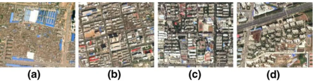
We examine the relationship between neighborhood form and household travel energy use in Jinan, China. Jinan is the capital city of Shandong Province, with a registered population of approximately 6.09 million as of the end of 2012 (Statistics Bureau of Jinan 2013). Lying on the lower reaches of the Yellow River and positioned near the east coast of China, Jinan is a historically and culturally rich city, first established more than 4,000 years ago. We selected nine neighborhoods representing four different urban form typologies commonly found in Chinese cities: traditional, grid, enclave and superblock, as shown in Fig. 1. Each represents characteristics of local urban development during sequential historic periods. A summary of the nine neighborhood cases and the features associated with each typology are shown in Table 1. Figure 2 shows the locations of these neighborhoods. 3.2 Household survey

In mid- 2009, a team from Shandong University carried out a survey, using the nine neighborhoods identified as the sampling frame. Households were selected, without replacement, using stratified random sampling based on building volumes within the neighborhoods. Eligible respondents were adults, aged 20 to 65 years, who resided in private dwellings such as houses or apartments. Respondents were interviewed at home by the enumerators. At the beginning of the survey, participants were asked to provide a detailed travel diary of each family member during the past full week, including weekends. Specific travel-related information requested included trip purpose,

Fig. 1 The study examined energy use data for four neighborhood typologies: a traditional, b grid, c enclave, and d superblock

E m TD

i

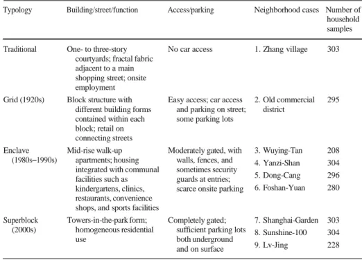
Table 1 Summary of form features across four neighborhood typologies and nine neighborhood cases in China Typology Building/street/function Access/parking Neighborhood cases Number of

household samples Traditional One- to three-story

courtyards; fractal fabric adjacent to a main shopping street; onsite employment

No car access 1. Zhang village 303

Grid (1920s) Block structure with different building forms contained within each block; retail on connecting streets

Easy access; car access and parking on street; some parking lots

2. Old commercial district 295 Enclave (1980s–1990s) Superblock (2000s) Mid-rise walk-up apartments; housing integrated with communal facilities such as kindergartens, clinics, restaurants, convenience shops, and sports facilities Towers-in-the-park form;

homogeneous residential use

Moderately gated, with walls, fences, and sometimes security guards at entries; scarce onsite parking

Completely gated; sufficient parking lots both underground and on surface 3. Wuying-Tan 208 4. Yanzi-Shan 304 5. Dong-Cang 296 6. Foshan-Yuan 280 7. Shanghai-Garden 303 8. Sunshine-100 304 9. Lv-Jing 228

Based on Massachusetts Institute of Technology and Tsinghua University (2010)

trip frequency, average trip distance for each purpose (in kilometers), and trip mode. The survey also collected information on household socioeconomics, demographics (gender, age, income, and occupation for each family member), housing tenure type, and vehicle ownership (cars, motorcycles, e-bikes, and bicycles). At the end of the survey, respondents were asked to rate four Likert-scale statements based on their level of agreement with each statement. These statements included: Car ownership is a sign of prestige; taking public transit is convenient; I enjoy bicycling; and time spent on travel is a waste of time. Each statement had five response levels: strongly disagree, partially disagree, neutral, partially agree, and strongly agree; these were coded 1, 2, 3, 4, and 5, respectively. A total of 2,660 eligible participants from the nine neighborhoods filled out the survey questionnaires; 2,521 of them provided consistent and generally complete information. The distribution of the sample across nine neighborhood cases is presented in Table 1.

3.3 Energy use estimates

Using the reported weekly travel diary data, we calculated the estimated weekly transportation energy consumption of each household in our sample. We summed up the household weekly distance travelled using each mode of transportation and adjusted for occupancy per trip. Then we converted the distances per mode into energy consumption by multiplying by the mode’s energy intensity. The energy intensity is calculated using the vehicle’s fuel economy and the fuel energy content factor, as follows:

m X X i ¼ FRi; j;k m ! i; j;k * _m * EIm _ð2Þ ET i ¼ X

Em; mj∈fcakr; taxi; bus;OmCoi; jt;ok rcycle; ebikeg ð1Þ m

ET

i,j,k

OCi,j,k

i

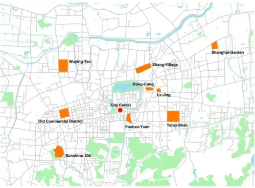
Fig. 2 Location of nine neighborhood case locations, each corresponding to one of the four neighborhood typologies, Jinan, China

where

EIm ¼ FUm * ECm ð3Þ

i Total household weekly transport energy consumption, by household i, in

megajoules per household per week (MJ/HH/week)

m

Weekly household transport energy consumption, by household i using mode m, in megajoules per household per week (MJ/HH/week)

m _{Trip frequency (trips/week), by mode m, for purpose k, by person j in household i}

FRi,j,k

TD m _{Average travel distance per trip (km/trip), by mode m, for purpose k, made by}

person j in household i

m

Trip occupancy, by mode m for purpose k, by person j in household i

EIm Energy intensity factor for mode m (MJ/km)

FUm _{Fuel consumption factor in liters per kilometer or kilowatt-hours per kilometer}

(L/km; kwh/km) associated with mode m; and

ECm _{Energy content factor in megajoules per liter (MJ/L) of the fuel type consumed}

by mode m.

Occupancy rates of the automobiles, taxis, motorcycles, and e-bikes can be associated with each trip and thus were estimated using reported person-trip data from the survey. Specifically, person-trips with exactly the same reported purpose, length, and time for two or more

Table 2 Fuel consumption, fuel energy content, and energy intensity assumptions in the study

Mode Fuel consumption Fuel energy content, MJ/L Energy intensity factor, MJ/km

Car 0.092 L/km 32.2 2.96

Taxi 0.083 L/km 32.2 2.67

Bus 0.3 L/km 35.6 10.68

Motorcycle 0.019 L/km 32.2 0.61

E-bike 0.021 kwh/km – 0.08

Based on National Bureau of Statistics (2008); Cherry et al. (2009); Guo et al. (2014)

household members were treated as one trip shared by all. Table 2 presents the average fuel consumption and energy consumption data used in the analysis.

3.4 Analytical approach

Descriptive statistics help depict household travel patterns and associated energy use and emissions, and they also help to understand whether and how those patterns differ across neighborhood typologies. We aggregated household transport energy usage levels at both the neighborhood case level and the typology level. In other words, we calculated the average household transport energy usages for households living within each of the nine neighbor- hoods, as well as the average for households living in each of the four typologies. Then we compared the neighborhood-level numbers with each other and compared the typology numbers with reported average transport energy usage in other regions of the world.

To further separate the effect of neighborhood form on energy use from confounding factors such as household socio-demographics, estimating econometric models is warranted. While standard one-step multivariate regression analyses were straightforward and widely applied in previous studies, we faced a classic challenge for a more rigorous causality study. The challenge is often referred to as self-selection associated with two related forms of bias: simultaneity bias and omitted variable bias (Mokhtarian and Cao 2008; Zegras 2010). In our case specifically, simultaneity bias means that households may choose to live in the super- blocks or buy cars, simply (or at least simultaneously) because they are addicted to an energy- intensive travel pattern (e.g., car prestige). To correct this, we collected attitudinal information in the household survey and included it in the regression model as a control variable.

Omitted variable bias may be present at the same time as we also want to separate the effect of neighborhood form on energy use from its influence on car ownership. Consider that we specify one-step multivariate regression analyses of household travel energy use with both neighborhood form and car ownership included as explanatory variables. The car ownership variable may be correlated with unobserved variables (the destination features, for example), which also produce the travel energy use outcomes. Now that the presumed exogenous car ownership variable becomes endogenous, it can produce inconsistent and biased estimators.

Approaches to control for self-selection, as summarized by Cao et al. (2009), include direct questioning, statistical control, instrumental variables, sample selection, propensity score, joint discrete choice models, structural equations models, mutually dependent discrete choice models, and longitudinal designs. In this research, we have developed two-step instrumental variable models, using relevant instruments to predict the car ownership odds first and then replacing the observed car ownership odds in the second-stage equation with their predicted values from the first-stage model. Adapted from the method by Zegras (2010), these predicted car ownership odds, in theory, purge the independent choice variable (in this case, the observed

i

ET

dummy variable indicating whether a household has at least one car) of its correlation with the error term and thus would correct the self-selection and endogeneity problems.

In the first step, we regress household car ownership using instrumental variables. Because the vehicle ownership variables are discrete (1 for households owning vehicles, and 0 otherwise), the binary logistic regression model is the appropriate model type; it takes the following form:

1

Pi ¼

1 e−ui ð4Þ

where P1 =the probability of a household owning one or more cars, and P2 =the probability

of a household owning no cars.

In the second step, we estimate the regression as usual, except that vehicle ownership values are replaced with the predicted ownership values from the logistic regression. The conventional multivariate ordinary least squares (OLS) regression analysis is performed using the log- transformed energy consumption rates for household weekly travel based on variables that include neighborhood form measurements and the disaggregated household-level data. This result is not problematic in the context of the developed world, where we may expect that recorded transpor- tation energy use values are rarely zero, given that most households either drive cars or take public transit. In China, however, a substantial portion of the population still does not have access to automobiles and may only be able to walk and bike. In those cases, household energy consump- tion will be recorded as a zero value, which may be qualitatively different from a random zero. In other words, those households may intentionally choose to have zero energy use and might even prefer to choose negative energy use. Given that negative energy use is impossible in this context, the subsequent fitting of an OLS regression line to all of the observations, including the zeroes, may underestimate the actual relationship between the independent variables and energy use. The statistics literature refers to this as a censoring problem of the dependent variable.

In this situation, a TOBIT model, first developed by Tobin (1958), is an appropriate method. The TOBIT model assumes that, for each observation, there is a latent variable

i*, which linearly depends on a vector of independent variables Xi with a normally

distributed error term εi (Sigelman and Zeng 1999):

ET i* ¼ β

0

* X i þ εi ð5Þ

Using TOBIT, the observed variable Ei equals the latent variable whenever ET * is greater

than zero, and zero otherwise: ₍

T * _{if E}T * _{> 0} ET i ¼ E i i ð6Þ 0 if ET i* ≤ 0 4 Results 4.1 Comparative analysis

As illustrated in Fig. 3, the superblock is associated with the highest level of household transportation energy consumption among the four typologies. The gap between the super- block and other typologies results from the much higher amounts of energy used by automo- biles. To place these estimates into a broader context, we compare the calculated personal annual travel energy use in Jinan with similar figures for international cities. As shown in Fig. 4, the current level of energy use for passenger travel in Jinan is still much lower than the level in cities of developed countries, even when compared with values from 1995. However,

MJ/ household 25000 20000 15000 10000 5000 000 E-bike Motorcycle Transit (incl. shuttle) Taxi Car (incl. company car)

Fig. 3 Average annual household transport energy use in nine neighborhoods in Jinan, China according to transport mode

the average person in a superblock consumes travel energy at a level close to the average in affluent cities in Asia and at a level higher than residents in most cities in the developing

Fig. 4 An international comparison of personal annual transport energy use shows 2009 values for Jinan and 1995 values in other countries. USA refers to U.S. cities; ANZ refers to Australia/New Zealand cities; CAN refers to Canadian cities; WEU refers to western European cities; HIA refers to high-income Asian cities; EEU refers to Eastern European cities; MEA refers to Middle Eastern cities; LAM refers to Latin American cities; ARF refers to African cities; LIA refers to low-income Asian cities; CHN refers to Chinese cities (Kenworthy 2008)

23170 23657 21179 10633 8484 7439 6175 7352 4852

Enclave Superblock Grid Traditional

D ong -C a ng W uy in g -T a n F os ha n -Y ua n Yanz i-S ha n Lv -J in g Suns hin e 1 00 Sha ng hai Ga rde n C om m erc ial D is tric t Z han g Vil la ge

world. Interestingly, the per-capita passenger energy consumption in Jinan’s non-superblock neighborhoods today is not much different from the average energy consumed in Chinese cities more than a decade ago.

We then investigate 502 zero-value cases in the sample, which represent super-efficient transportation energy households. The share of such type of households in the superblock is only 5 %, whereas the shares in the other neighborhood typologies are as high as 24 to 35 %. This observation again suggests that the superblock is much less energy efficient than an average of all other neighborhood types from the household travel point of view.

4.2 Two-step instrumental variable models

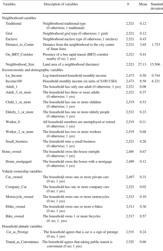
We now examine weekly household travel energy consumption in an attempt to identify the relative role of neighborhood typology and location features after controlling for potentially confounding variables. In our analysis, we specify a number of models. The dependent variable for the first-stage models is a dummy variable of value 1 for households owning one or more cars, and value 0, otherwise. The dependent variable for the second-stage model is the adjusted log-transformed household weekly transport energy use. Table 3 presents the variables and their descriptive statistics from the sample. Note that numbers of observations vary across variables due to some cases with incomplete answers to pertinent questions.

4.2.1 First stage: car ownership models

For the regression of car ownership, we use an incremental model specification approach. The basic model is a control model that includes only household socioeconomic and demographic variables and other vehicle ownership variables. In the next model specification, we include the neighborhood variables. Last, we add the household attitude variables to arrive at the full model (plus attitude). Table 4 reports the results.

The significance and signs of explanatory variables remain consistent across the three models. Inserted instrumental variables are all significant at the 0.05 level, except for the variable that represents attitudes favoring biking. This result suggests that the car ownership model can be used to instrument the second-stage model of energy use.

The final plus attitude model exhibits the best goodness of fit among all three models, evidenced by an application of the likelihood ratio test. Therefore, we use this full model to calculate the predicted values of car ownership for each household. In the second-stage model, these predicted values replace observed car ownership values to correct for the endogeneity problem in single-stage models.

The results suggest that neighborhood form characteristics may play an important role in affecting household car ownership choice after controlling for confounding factors, including attitudes. The signs of the coefficients for all three dummy variables for non-superblock neighborhood typology are negative, suggesting that households living in the superblock neighborhoods have a higher probability of car ownership. This result may be attributed to the difference between the automobile-oriented design features of superblock neighborhoods, compared with the more pedestrian-oriented design of the other neighborhood typologies. Travel attitudes figure significantly in the model, which we discuss below, so we can assert at least partial control for the possibility that automobile-oriented households prefer to live in the superblocks. The variable effects for neighborhood form are significant even after controlling for attitudes. The neighborhood size coefficient shows a positive sign, indicating that house- holds living in larger neighborhoods are more likely to own cars. An explanation might be that neighborhoods in Jinan often do not have public transit service within their boundaries, except

Table 3 Descriptive statistics of variables in the study sample

Variables Description of variables N Mean Standard

deviation Neighborhood variables

Traditional Neighborhood traditional type (0 otherwise; 1 traditional)

2,521 0.12 Grid Neighborhood grid type (0 otherwise; 1 grid) 2,521 0.12 Enclave Neighborhood enclave type (0 otherwise; 1 enclave) 2,521 0.43 Distance_to_Center Distance from the neighborhood to the city center

of Jinan (km)

2,521 3.65 1.753 On_BRT_Corridor Presence of a bus rapid transit (BRT) corridor 2,521 0.41

nearby (0 no; 1 yes)

Neighborhood_Size Land area of a neighborhood (hectares) 2,521 27.13 15.506 Socioeconomic and demographic variables

Ln_Income Log-transformed household monthly income 2,473 6.50 0.744 Income100 Household monthly income (in units of $100 USD) 2,473 8.58 6.321 Adult_1 The household has only one adult (0 otherwise; 1 yes) 2,521 0.08 Adult_3_or_more The household has three or more adults

(0 otherwise; 1 yes)

2,521 0.37 Child_1_or_more The household has one or more children 2,519 0.53

(0 otherwise; 1 yes)

Elderly_1_or_more The household has one or more elderly people 2,521 0.23 (0 otherwise; 1 yes)

Worker_0 All household members are unemployed or retired 2,519 0.11 (0 otherwise; 1 yes)

Worker_2_or_more The household has two or more workers 2,519 0.68 (0 otherwise; 1 yes)

Small_business The household runs a small business 2,521 0.26 (0 otherwise; 1 yes)

Home_owned The household owns the house outright (0 otherwise; 1 yes)

2,489 0.67 Home_mortgaged The household owns the house with a mortgage

(0 otherwise; 1 yes)

2,489 0.12 Vehicle ownership variables

Car_owned The household owns one or more private cars (0 no; 1 yes)

2,497 0.31 Company_Car The household has one or more company cars

(0 no; 1 yes)

2,521 0.02 Motorcycle_owned The household owns one or more motorcycles

(0 no; 1 yes)

2,515 0.10 Ebike_owned The household owns one or more e-bikes

(0 no; 1 yes)

2,511 0.36 Bike_owned The household owns 1 or more bicycles 2,517 0.57 Household attitude variables

(0. no; 1. yes)

Car_as_Prestige The household agrees that a car is a sign of prestige (0 no; 1 yes)

Transit_as_Convenience The household agrees that taking public transit is convenient (0 no; 1 yes)

2,519 0.24 2,520 0.66

Table 3 (continued)

Variables Description of variables N Mean Standard

deviation I_Like_Biking The household agrees that I enjoy bicycling

(0 no; 1 yes)

2,515 0.54 Travel_is_Waste_ The household agrees that time spent traveling 2,520 0.41

of_Time is a waste of time (0 no; 1 yes)

in the superblock type. The size of a neighborhood may be correlated with the average walking distance for access to public transit among residents. In larger neighborhoods, public transit may be less accessible, and as a result, residents may shift toward driving and owning cars.

Neighborhood location characteristics matter as well. The model results indicate that car ownership tends to be higher for households living close to the city center, compared with those who live farther away. This result is contrary to most findings in Western countries, yet it is consistent with recent findings in Beijing and Chengdu, China, by Li et al. (2010). The authors of that article argue that urban centers in most Chinese cities provide good urban amenities, and residents in households with cars are often wealthy and still prefer to live there; in the United States; however, middle class and affluent families tend to prefer suburban communities and avoid city centers that have declined since World War II. This argument, although valid to some extent, may not be convincing given that the authors already control for household income in their models. In our case, we speculate that the observed effect of the distance to the city center may be because (1) there is little variation in the distance to city center among the neighborhoods studied, or (2) the variable of the distance to the city center itself is not a good proxy for measuring regional accessibility, given that Jinan has already evolved into more of a multi-center city structure.

The effect of proximity to bus rapid transit (BRT) corridors on household car ownership reveals some potentially interesting dynamics. In the plus-neighborhood model, the results suggest that the effect is significant and negative. However, this effect becomes insignificant after controlling for household attitudes in the plus-attitude model. This change in significance, combined with the revealed negative and significant effects of attitudes toward public transit convenience, suggests a self-selection effect is occurring: Households may live on the BRT corridor because their members like public transit, and this travel mode preference is so strong that it lowers their likelihood of owning cars.

Household characteristics also exhibit some notable effects. The effect of household income is positive, as expected: Wealthier households have a higher probability of owning cars. Having children may be an incentive for households to buy cars, whereas the opposite effect is present in households consisting of elderly people. These results align with what one would intuitively expect, because walking, biking, or taking public transit with children is often inconvenient and unsafe. For elderly people, driving may become more difficult than taking other modes of transportation, or elderly people may simply have different lifestyle habits and expectations. The number of workers in a household has a positive impact on car ownership. Households running a small business are more likely to own a car, probably reflecting the demand for flexibility and logistics in their businesses. Homeowners who have no mortgage debt have a higher chance of owning a car than households owning a house with a mortgage; renter households have the lowest likelihood of car ownership. Renters or mortgage payers have less disposable income relative to homeowners without mortgages. Family size does not have a significant effect on car ownership. Ownership of other types of

Table 4 Binary logistical regression models predicting car ownership in the Jinan, China study Control model Plus neighborhood Plus attitudes Coefficient Z-test Coefficient Z-test Coefficient Z-test

Household characteristics Income_100USD 0.139a _{12.44 0.105}a _{9.11 0.099}a _8.45 Adult_1 Adult_2 0.216 Ref.c 0.73 0.034 Ref.c 0.11 −0.027 Ref. −0.09 Adult_3_or_more −0.196 −1.49 −0.095 −0.69 −0.052 −0.38 Child_1_or_more 0.491a _{5.04 0.423}a _{4.18 0.431}a _4.20 Elderly_1_or_more −0.495a _{−3.22 −0.429}a _{−2.68 −0.383}a _−2.36 Worker_0 −1.378a _{−4.70 −1.248}a _{−4.18 −1.148}a _−3.82 Worker_1 Worker_2_or_more −0.478a Ref.c −3.03 −0.448a Ref.c −2.74 −0.399a Ref. −2.40 Company_car −0.094 −0.28 −0.128 −0.38 −0.223 −0.66 Motorcycle_owned −0.698a −3.55 −0.577a −2.81 −0.577a −2.80 Ebike_owned −0.669a −5.92 −0.675a −5.74 −0.714a −5.98 Bike_owned −0.785a −7.18 −0.724a −6.35 −0.711a −6.07 Small_business 0.366a _{3.01 0.379}a _{2.97 0.361}a _2.79 Home_owned 1.601a _{8.60 1.391}a _{6.84 1.425}a _6.97 Home_mortgaged 1.726a _{7.86 1.059}a _{4.21 1.057}a _4.16 Neighborhood characteristics Distance_to_Center On_BRT_Corridor Neighborhood_Size Traditional Grid Enclave Superblock −0.163a −0.249b 0.013a −1.212a −1.660a −1.684a Ref.c −3.82 −1.66 2.93 −4.04 −7.22 −8.90 −0.151a −0.231 0.011a −1.106a −1.522a −1.535a Ref.c −3.46 −1.52 2.52 −3.64 −6.52 −7.98 Household attitudes Car_as_Prestige

a _{Denotes statistical significance at 5 % level} b _{Denotes statistical significance at 10 % level} c _{Denotes reference case}

vehicles lowers the probability of owning cars, indicating a substitution effect among different choices in vehicle type.

Finally, attitudes have critical impacts on car ownership. Households that see a car as a sign of prestige are less likely to own cars. This result can be interpreted in two ways: (1) households without cars envy those who have one (a sign of car prestige/status effect), and (2) as households purchase cars, car ownership comes to be perceived more as a need than as a sign of status. Perceiving public transit as a convenient mode of transportation decreases the household’s likelihood of owning cars, suggesting that public transit serves as at least a partial substitute for driving in Jinan. Finally and most notably, households viewing travel as a waste of time are more likely to own cars, an observation that implies that these households place a higher value on time and thus prefer the speed and convenience of car ownership.

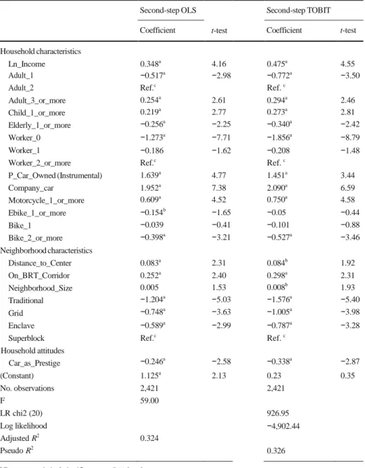
4.2.2 Second stage: vehicle use energy models

In the second-stage model, we first predict car ownership probabilities for all observations in our sample and insert these predicted values into the initial regression equation for the weekly total travel energy use per household, replacing the observed car ownership values. We test both the OLS and TOBIT models for the regression of travel energy consumption. Table 5

compares the results from these two approaches.

Significance and signs of the coefficients for most explanatory variables are almost the same across the two models. With respect to the neighborhood characteristics, the coefficients of the three neighborhood typology dummy variables are all negative and significant at the 5 % level, which gives us confidence in concluding that households in the traditional, grid, and superblock neighborhoods consume less energy in traveling than those living in the superblock neighborhoods. Diverse land use, parking restrictions, and walkable street design (i.e., a refined internal road network) may encourage households to travel with higher energy efficiency in these neighborhoods. The only neighborhood characteristic that has a non- significant effect is the neighborhood size. In both models, living on BRT corridors is strongly associated with higher energy consumption for travel. This result may seem counterintuitive, but it can be explained by tradeoffs among different types of travel patterns; we discuss these tradeoffs in the conclusion. We are also quite confident that the distance to the city center has a positive effect on household energy use, despite having a less significant effect in the second- stage TOBIT model. The reason could be that neighborhoods farther away from the center, with all else being equal, are also geographically farther from all other potential destinations in the city—assuming an urban center-to-periphery density gradient—and have lower access to mass transit and nearby public services. The effect of neighborhood size is also significant at the 10 % confidence level, after correcting for censoring and endogeneity problems by using the two-stage TOBIT model. Our statistical control on the neighborhood size may thus be effective.

Regarding socioeconomic variables, most are significant with expected signs. For example, the significant and positive coefficient of the log-transformed income variable suggests a positive effect, with diminishing returns, of income on household travel energy use. In other words, the wealthier a household is, the more travel energy it consumes, but it consumes less as it becomes even wealthier. This result is also intuitive, given that people have time, budget, and physical constraints. Families with children consume more travel energy, whereas aging families consume less. The reason for this contrast may be that children raise the overall household travel demand, because they require additional travel to recreation, education, and healthcare activities. In contrast, elderly people may be more physically constrained or may have fewer commitments outside of the home and thus prefer to stay at home or travel short distances.

Table 5 Comparisons of models predicting log-transformed household weekly total travel energy use

Second-step OLS Second-step TOBIT

Coefficient t-test Coefficient t-test

Household characteristics Ln_Income 0.348a _{4.16 0.475}a _4.55 Adult_1 Adult_2 Adult_3_or_more −0.517a Ref.c 0.254a −2.98 2.61 −0.772a Ref. c 0.294a −3.50 2.46 Child_1_or_more Elderly_1_or_more Worker_0 0.219a −0.256a −1.273a 2.77 −2.25 −7.71 0.273a −0.340a −1.856a 2.81 −2.42 −8.79 Worker_1 Worker_2_or_more P_Car_Owned (Instrumental) −0.186 Ref.c 1.639a −1.62 4.77 −0.208 Ref. c 1.451a −1.48 3.44 Company_car 1.952a _{7.38 2.090}a _6.59 Motorcycle_1_or_more Ebike_1_or_more 0.609a −0.154b 4.52 −1.65 0.750a −0.05 4.58 −0.44 Bike_1 Bike_2_or_more −0.039 −0.398a −0.41 −3.21 −0.101 −0.527a −0.88 −3.46 Neighborhood characteristics Distance_to_Center 0.083a _{2.31 0.084}b _1.92 On_BRT_Corridor 0.252a _{2.40 0.298}a _2.31 Neighborhood_Size Traditional Grid Enclave Superblock 0.005 −1.204a −0.748a −0.589a Ref.c 1.53 −5.03 −3.63 −2.99 0.008b −1.576a −1.005a −0.787a Ref. c 1.93 −5.40 −3.98 −3.28 Household attitudes Car_as_Prestige −0.246a −2.58 −0.338a −2.87 (Constant) 1.125a _{2.13 0.23 0.35} No. observations 2,421 2,421 F 59.00 LR chi2 (20) 926.95 Log likelihood Adjusted R2 Pseudo R2 0.324 −4,902.44 0.326 a

Denotes statistical significance at 5 % level

b _{Denotes statistical significance at 10 % level} c _{Denotes reference case}

Not surprisingly, vehicle ownership variables have significant impacts on energy use as well. Households with cars use more energy, and households with a company car in particular tend to consume more energy than those with a private car. This observation is in line with previous empirical findings by Huo et al. (2012). It implies that company cars induce more

automobile use, possibly because company car drivers do not pay for the fuel. These household members may also be assigned company cars because of their intensive business travel requirements.

Finally, out of the five attitude variables, only the effect of the attitude relating to car prestige or status is revealed to be significant. This variable’s coefficient is negative, suggest- ing that, all else being equal, households that view the car as a sign of prestige do consume less travel energy, and vice versa. As suggested in the vehicle ownership model above, one possible explanation is that people who have a car and drive frequently in Jinan today regard it as a common means of travel. Such a finding may also imply, however, that among people without much driving experience, the status symbol perception still exists and may serve as a strong motivation for their future transition to car ownership.

5 Conclusions and policy implications

Rapidly increasing transportation energy use in China poses challenges to national energy security and to the mitigation of GHG emissions at the global scale. Meanwhile, automobile- oriented neighborhood development, such as the development of superblock housing, domi- nates current urban expansion and construction in Chinese cities. This paper provides a pilot empirical study of relationships between neighborhood form and transport energy use in the context of Jinan, China. Household transportation energy uses are derived from households’ self-reported, weekly travel diaries. These diaries were collected using a household survey in nine neighborhoods, which represent the four types of urban communities commonly found in Chinese cities: traditional, grid, enclave, and superblock. Comparative analysis and two-step instrumental variable models suggest that, all else being equal, households living in superblock neighborhoods consume more transportation energy than those living in the other neighbor- hood types, as residents in superblock neighborhoods tend to own more cars and travel longer distances. A number of effects caused by neighborhood location, household socioeconomics, demographics, and attitudes about transportation energy use and car ownership are also identified.

On the basis of these results, we make five policy recommendations to help chart a more energy-efficient future in urban China. First, past neighborhood designs must be examined to find alternatives to the currently popular superblock. Our study reveals that pre-2000s neigh- borhood typologies in Jinan are associated with 65–80 % less household travel energy use than the superblock. The potential for energy reduction may come from lower vehicle usage as well as lower probability of car ownership, most likely resulting from the mixed land uses, as well as an environment friendly to non-motorized transport, implicit traffic-calming measures, and parking restrictions in these neighborhoods. Although these principles were not necessarily intended to save energy when the neighborhoods were initially built, they could be revisited to inspire policymakers and urban planners in the process of formulating rules, regulations, and guidelines and inventing new neighborhood typologies for future urban development in China. Second, using strategic infill development to accommodate urban growth would likely mitigate transport energy use in China. Our analysis demonstrates that greater distance to the city center is positively related to higher travel energy consumption. On the other hand, the evidence that households living next to BRT corridors consume even more transportation energy may trigger some controversy on whether cities should have more transit corridors. We believe transit corridors can indeed help households enjoy more opportunities without being more car-dependent, as partly evidenced by the BRT corridors’ modest negative effect on household car ownership in our model. The real challenge is that transit corridors in China are

often designated together with expressways or wide arterials, which tend to offer more incentives to car driving than to riding transit. Thus, it seems equally important to create true transit-oriented corridors that eventually deliver benefits.

Third, promoting the growth of bicycles and e-bikes as a substitute for larger motorized vehicles deserves particular attention in developing transport policies from an efficient energy perspective. While rapid motorization is often regarded as increasing car ownership, the rise of motorcycle and e-bike ownership in China is also phenomenal. Our data from Jinan suggest that households owning private cars and motorcycles consume more energy than households that do not own vehicles. Meanwhile, company cars, a unique vehicle type quasi-owned by households, account for a strong effect on energy use at the household level among all vehicle types, including private cars. Thus, better monitoring or more restrictive company car use rules may be helpful in reducing household travel energy consumption.

Fourth, improving the efficiency of public transportation could be desirable as well. The empirical evidence shows that the magnitude of transit energy use is currently comparable with that of car energy use in Chinese cities like Jinan. Although more efficient transit systems may be derived from cleaner fuel or better bus engine design, improving the transit system’s operations (i.e., scheduling) may be equally effective. In addition, policies for boosting transit ridership can make the system more energy efficient by increasing occupancy and therefore lowering the amount of system-wide energy use per passenger-kilometer.

Finally, programs for shaping traveler preferences may present additional opportunities for mitigating transportation energy use or GHG emissions. Echoing findings by Zhao (2009), our analysis in Jinan shows that people’s attitudes toward different travel modes do indeed have significant impacts on automobile ownership, a main driver of transportation-related energy consumption growth in China. However, our study also found that those preferences have little effect on vehicle use, after controlling for ownership. These observations imply that shaping preferences in China, if appropriately done, can be an effective measure to slow the process of rapid motorization; nevertheless, the window for implementing such policies is quickly shrinking.

Acknowledgments This work is supported by the Energy Foundation, the Low Carbon Energy University Alliance (No. 2011LC002), and the National Natural Science Foundation of China (No.51378278). We acknowledge our research partners at Tsinghua University, Shandong University, Beijing Normal University, and Massachusetts Institute of Technology. Specifically, we thank Prof. Dennis Frenchman for identifying the four neighborhood typologies in Jinan; Prof. Zhang Ruhua and Prof. Zhang Lixin for organizing local survey work; and Yang Chen for data cleaning. We also thank Dr. Jinhua Zhao, Dr. Michael Wang, and three anonymous referees for valuable comments and suggestions.

References

BP (2013) BP statistical review of world energy June 2013. http://www.bp.com/content/dam/bp/pdf/statistical- review/statistical_review_of_world_energy_2013.pdf. Cited June 2013

Cao X, Mokhtarian P, Handy S (2009) Examining the impacts of residential self selection on travel behaviour: a focus on empirical findings. Transp Rev 29(3):359–395

Cervero R, Day J (2008) Suburbanization and transit-oriented development in China. Transp Policy 15(5):315–323 Chen R, Wang J (2007) Energy and transportation: a case study in China. IEEE Intell Syst 22(3):10–12 Cherry CR, Weinert JX, Xinmiao Y (2009) Comparative environmental impacts of electric bikes in China.

Transp Res D 14:281–290

Cheslow MD, Neels JK (1980) Effect of urban development patterns on transportation energy use. Transp Res Rec 764:70–78

Darido G, Torres-Montoya M, Mehndiratta S (2013) Urban transport and CO2 emissions: some evidence from

Emrath P, Liu F (2008) Vehicle carbon dioxide emissions and the compactness of residential development. Cityscape: J Policy Dev Res 10(3):185–202

Frank LD, Stone B, Bachman W (2000) Linking land use with household vehicle emissions in the central Puget Sound: methodological framework and findings. Transp Res D 5:173–196

Frank LD, Greenwald MJ, Winkelman S, Chapman J, Kavage S (2009) Carbonless footprints: promoting health and climate stabilization through active transportation. Prev Med 50(1):99–105

Guo J, Liu H, Jiang Y, He D, Wang Q, Meng F, He K (2014) Neighborhood form and CO2 emission: evidence

from 23 neighborhoods in Jinan, China. Front Environ Sci Eng 8(1):79–88

Handy S (1996) Methodologies for exploring the link between urban form and travel behavior. Transp Res D 1(2):151–165

He K, Huo H, Zhang Q, He D, An F, Wang M, Walsh MP (2005) Oil consumption and CO2 emissions in China’s

road transport: current status, future trends, and policy implications. Energy Policy 33(12):1499–1507 Holden E, Norland IT (2005) Three challenges for the compact city as a sustainable urban form: household

consumption of energy and transport in eight residential areas in the greater Oslo region. Urban Stud 42(12): 2145–2166

Hong J, Shen Q (2013) Residential density and transportation emissions: examining the connection by addressing spatial autocorrelation and self-selection. Transp Res D 22:75–79

Huo H, Zhang Q, He K, Yao Z, Wang M (2012) Vehicle-use intensity in China: current status and future trend. Energy Policy 43:6–16

International Energy Agency (2007) World energy outlook 2007: China and India insights. International Energy Agency, Washington

Kenworthy JR (2008) Energy use and CO2 production in the urban passenger transport systems of 84

international cities: findings and policy implications. In: Droege P (ed) Urban energy transition: from fossil fuels to renewable power. Elsevier, London, pp 211–236

Li JP, Walker JL, Srinivasan S, Anderson WP (2010) Modeling private car ownership in China: investigating the impact of urban form across mega-cities. J Transp Res Board 2193:76–84

Massachusetts Institute of Technology, Tsinghua University (2010) Making the clean energy city in China: year 1 report. Submitted to Energy Foundation, Massachusetts Institute of Technology

Mokhtarian PL, Cao X (2008) Examining the impacts of residential self-selection on travel behavior: a focus on methodologies. Transp Res B 42(3):204–228

Monson K (2008) String block vs superblock patterns of dispersal in China. Archit Des 78(1):46–53

Naess P (2010) Residential location, travel, and energy use: the case of Hangzhou metropolitan area. J Transp Land Use 3(3):27–59

Naess P, Sandberg SL (1996) Workplace location, modal split, and energy use for commuting trips. Urban Stud 33(3):557–580

National Bureau of Statistics (2008) China statistical yearbook 2008. China Statistics Press, Beijing Newman WG, Kenthworthy JR (1989) Gasoline consumption and cities. J Am Plan Assoc 55:24–25

Norman J, MacLean H, Kennedy C (2006) Comparing high and low residential density: life-cycle analysis of energy use and greenhouse gas emissions. J Urban Plann Dev 132(1):10–21

Pan H, Shen Q, Zhang M (2009) Influence of urban form on travel behaviour in four neighbourhoods of Shanghai. Urban Stud 46(2):275–294

Sigelman L, Zeng L (1999) Analyzing censored and sample-selected data with Tobit and Heckit models. Polit Anal 8(2):167–182

Statistics Bureau of Jinan (2013) Jinan statistical yearbook 2013. China Statistics Press, Beijing

Stone B, Mednick AC, Holloway T, Spak SN (2007) Is compact growth good for air 1uality? J Am Plan Assoc 37:404–418

Tobin J (1958) Estimation of relationships for limited dependent variables. Econometrica 26:24–36

VandeWeghe JR, Kennedy C (2007) A spatial analysis of residential greenhouse gas emissions in the Toronto census metropolitan area. J Ind Ecol 11(2):133–144

Wang D, Chai Y (2009) The jobs-housing relationship and commuting in Beijing, China: the legacy of Danwei. J Transp Geogr 17(1):30–38

Woetzel J, Joerss M, Bradley R (2009) China’s green revolution: prioritizing technologies to achieve energy and environmental sustainability. McKinsey & Company, Beijing

Zegras C (2010) The built environment and motor vehicle ownership and use: evidence from Santiago de Chile. Urban Stud 47(8):1793–1817

Zhao J (2009) Preference accommodating and preference shaping: incorporating traveler preferences into transportation planning. Dissertation, Massachusetts Institute of Technology